


| Issue |
A&A
Volume 710, June 2026
|
|
|---|---|---|
| Article Number | A31 | |
| Number of page(s) | 8 | |
| Section | Extragalactic astronomy | |
| DOI | https://doi.org/10.1051/0004-6361/202558454 | |
| Published online | 29 May 2026 | |
SDSS J153231.80+420342.7: A triple black hole candidate with a close binary black hole
1
School of Physics and Technology, Nanjing Normal University, No. 1 Wenyuan Road, Nanjing 210023, PR China
2
Guangxi Key Laboratory for Relativistic Astrophysics, School of Physical Science and Technology, Guangxi University, Nanning 530004, PR China
★ Corresponding authors: This email address is being protected from spambots. You need JavaScript enabled to view it.
, This email address is being protected from spambots. You need JavaScript enabled to view it.
Received:
8
December
2025
Accepted:
2
April
2026
Abstract
We reported a triple black hole candidate with a close binary black hole (BBH) in the blue quasar SDSS J153231.80+420342.7 (=SDSS J1532) at a redshift of 0.209. It shows double-peaked profiles in all narrow emission lines, which can be a signature of a dual active galactic nucleus (AGN). If the double-peaked features are produced by a dual AGN, the estimated physical separation between the two cores is about 3 kpc. Alternative interpretations to the double-peaked profiles involving models of rotating disk-like narrow-line regions (NLRs) and AGN-driven outflows are also discussed for the double-peaked features. In addition, SDSS J1532 shows optical quasiperiodic oscillations (QPOs) of about 0.6 yr from the ZTF and CSS light curves, with time duration that is longer than 14 years, which may indicate a binary black hole with ∼1 mpc separation. Two alternative models, disk precession and jet precession, are also discussed. The current results cannot completely rule out alternative models for the characteristics of the spectrum and light curves. As a candidate for a triple black hole with two cores in kiloparsec scale and a close BBH in milliparsec scale in SDSS J1532, it may be going through a critical period in its evolution.
Key words: galaxies: active / galaxies: nuclei / quasars: emission lines / quasars: supermassive black holes / quasars: individual: SDSS J153231.80+420342.7
© The Authors 2026
 Open Access article, published by EDP Sciences, under the terms of the Creative Commons Attribution License (https://creativecommons.org/licenses/by/4.0), which permits unrestricted use, distribution, and reproduction in any medium, provided the original work is properly cited.
This article is published in open access under the Subscribe to Open model. This email address is being protected from spambots. You need JavaScript enabled to view it. to support open access publication.
1. Introduction
Observational and theoretical studies have confirmed the presence of supermassive black holes (SMBHs) at the centers of most massive galaxies. Galaxy interactions are prevalent throughout the universe, and lead to hierarchical evolution through collisions (Toomre & Toomre 1972; Begelman et al. 1980; Silk & Rees 1998; Hopkins et al. 2005; De Rosa et al. 2023; Zheng et al. 2023). Consequently, the presence of multiple SMBHs in massive galaxies should be common. When the dual active galactic nuclei (AGNs) have projected separations of a few to several tens of kiloparsecs, the two nuclei can be directly imaged (Shen et al. 2019; Zheng et al. 2023). For more compact systems, double-peaked narrow emission lines (DPNELs), first introduced by Zhou et al. (2004) as indicators of dual AGNs at kiloparsec scales, have been widely used in systematic searches (Wang et al. 2009; Smith et al. 2010; Comerford et al. 2012; Ge et al. 2012; Liu et al. 2013; Kim et al. 2020).
In the later stages of galactic mergers, when two nuclei approach each other at subparsec distances, they form a binary black hole (BBH) system, potentially giving rise to the signature of periodic electromagnetic radiation variations on month or year timescales, due to the orbital motion of the two SMBHs. There are many candidates for BBH systems determined through quasiperiodic oscillations (QPOs) in different bands, as shown in Graham et al. (2015), Severgnini et al. (2018), Serafinelli et al. (2020), Millon et al. (2022), Zhang (2023), Foustoul et al. (2025), Huijse et al. (2025).
In even rarer scenarios, triple black holes may emerge when a third galaxy subsequently merges before the coalescence of the initial black holes (Valtonen 1996). To date, most candidates of triple black hole systems have shown projected separations of a few to tens of kiloparsecs (Barth et al. 2008; Liu et al. 2011; Kalfountzou et al. 2017; Pfeifle et al. 2019; Foord et al. 2021a,b; Peng et al. 2022), and only a few triple black hole candidates have the closest pairs separated by subkiloparsec distances. Deane et al. (2014) reported a triple black hole candidate, SDSS J150243.09+111557.3, with the closest pair separated by 140 pc and two components, which might be the reason for its double-peaked [O III] emission lines, separated by 7.4 kpc. However, the result of the closest pair was challenged by Wrobel et al. (2014), who thought that the radio components separated by 140 pc are double hot spots produced by a single SMBH. Kollatschny et al. (2020) reported the presence of three distinct nuclei within a 1 kpc region in the late-stage merger system NGC 6240, and revealed that the previously unresolved southern component is in fact composed of two separate nuclei, with a projected separation of merely 198 pc. Detecting pairs separated by such small distances through imaging is challenging, due to angular resolution limitations.
One potential indicator of much closer distances with subparsec relative separations is the detection of periodic electromagnetic radiation variations. Therefore, it may also be a promising method for searching for triple black hole systems by combining the DPNELs with QPO signatures.
For this paper we investigated SDSS J153231.80+420342.7 (=SDSS J1532), a triple black hole candidate selected from a sample of type 1 AGNs with double-peaked [O III] emission lines identified in the Data Release 16 of the Sloan Digital Sky Survey (Zheng et al. 2025). The virial black hole mass, estimated from the broad Hα emission line, is 108.68 ± 0.02 M⊙. In addition to the prominent double-peaked narrow emission-line profiles, SDSS J1532 shows evidence of QPOs in the optical band. These properties suggest that SDSS J1532 may have two compact cores separated by subparsec distances and a third core located at a kiloparsec-scale distance from them.
The structure of the paper is as follows. The data and methods used for SDSS J1532 are shown in Section 2. The results and discussions of possible physical models are presented in Section 3. The summary and conclusions are given in Section 4. We have adopted the cosmological parameters of H0 = 70 km/s/Mpc, ΩΛ = 0.7, and Ωm = 0.3.
2. Data and methods
2.1. Spectrum
SDSS J1532 is a typical QSO with broad emission lines at z ∼ 0.209. The processed and calibrated spectrum1 is from the Data Release 16 of the Sloan Digital Sky Survey (SDSS) (Ahumada et al. 2020); it is presented in the top left panel of Figure 1. This SDSS spectrum, obtained on MJD = 53149, was taken with a 2.5 m wide-field telescope using a fiber diameter of 3″, and covers the wavelength range 3794–9189 Å sampled by 3843 pixels. The spectral resolution is R ≈ 1800.
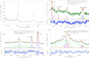 |
Fig. 1. Rest-frame optical spectrum of SDSS J1532 (top left panel) and best-fitting results of SDSS J1532 with rest-frame spectrum from 3850 Å to 4450 Å (top right panel), from 4750 Å to 5050 Å (bottom left panel) and from 6400 Å to 6800 Å (bottom right panel). In the top subpanels the solid dark green lines show the line spectra; the dashed blue and red lines represent the blueshifted and redshifted components of the narrow Hα, Hβ, Hγ, Hδ, He I, [Ne III], [O III], [N II], and [S II] doublets; the solid blue lines represent the extended components of the [O III] emission lines; the solid green lines represent the broad Hα, Hβ, and Hγ emission lines with the corresponding parameters of the central wavelength (Å), line width σ (Å), and line flux (10−17 erg/s/cm2) listed in the first two lines of the panels; the dashed cyan lines show the continuum emissions |
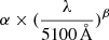
We focused on the main emission lines, spanning the rest wavelength from 3850 Å to 4450 Å, from 4600 Å to 5050 Å, and from 6250 Å to 6900 Å. The following model functions were used to describe these emission lines. A single power-law component was applied to describe the continuum emission underneath the Hγ, Hβ, and Hα emission lines. Two narrow Gaussian functions (the second moment σ < 400 km/s) were applied to describe the double-peaked profiles in each narrow emission line, and an additional Gaussian component (σ > 400 km/s) was included to model the wing component of [O III]. Finally, two broad Gaussian functions (σ > 800 km/s) were used to model the broad components of the Hγ, Hβ, and Hα lines. Here the positions of the emission lines were determined relative to their laboratory rest wavelengths (Vanden Berk et al. 2001).
The parameters were then constrained as follows. For the [O III], [N II], and [Ne III] doublets, the central wavelengths and line widths of the blueshifted and redshifted components were fixed with those of their respective companion lines within each doublet, and the flux ratio was set to the theoretical value of 3:1 (Storey & Zeippen 2000). For the [S II] doublet, the line width of the blueshifted and redshifted components was consistent with those of their respective companion lines in velocity space. The central wavelength of the blueshifted (redshifted) component of the Balmer narrow emission lines was fixed together in velocity space.
The main emission lines of SDSS J1532 were fitted using the Levenberg–Marquardt least-squares minimization method, as implemented in the MPFIT package (Markwardt 2009). The results (χ2/d.o.f. = 1.3, d.o.f. = 1373) are shown in Table 1. The peak separations and their associated uncertainties were derived from the central wavelengths and their corresponding uncertainties, and are also presented in Table 1. To clearly display the double-peaked profiles, portions of the rest-frame spectrum spanning 3850 Å–4450 Å, 4750 Å–5050 Å, and 6400 Å–6800 Å are shown in Figure 1 with the best-fitting model overplotted.
Features of main narrow emission lines.
2.2. Optical light curves
The Zwicky Transient Facility (ZTF; 47 deg2 field of view) (Bellm et al. 2019; Graham et al. 2019; Dekany et al. 2020), dedicated to surveying the transient and variable universe, operates on the 48-inch Samuel Oschin telescope at Palomar Observatory with three custom-made filters: ZTF-g, ZTF-r, and ZTF-i. The Catalina Sky Survey (CSS) (Drake et al. 2009), supported by the Near Earth Object Observation Program, is dedicated to the discovery and tracking of near-Earth objects. This survey is analyzed by the Catalina Real-Time Transient Survey to detect optical transient phenomena (V < 21.5 mag).
The optical-band photometric data of SDSS J1532 from ZTF (MJD: 58202-60489 for the g-band; 58198-60397 for the r-band; 58227-59985 for the i-band) and CSS (MJD: 53552-56563) are shown in Figure 2. Due to the lower quality of the CSS light curve, we only applied the epoch-folding method (discussed below) without conducting further analysis of its periodicity.
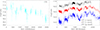 |
Fig. 2. Observed optical light curves of SDSS J1532 directly downloaded from the survey archives of the CSS (v-band) and ZTF (g-band, r-band, i-band). The solid and dashed lines show the best-fitting results and their corresponding 1RMS scatter bands, respectively. The dotted lines represent the results of the polynomial function. |
A simple sinusoidal function plus a six-degree polynomial function (a + bt + ct2 + dt3 + et4 + ft5 + gt6 + hsin(2πt/T + ϕ)) was applied to describe the three band light curves in ZTF with the same periodicity T. Here the sine component was only applied to show the periodic variability patterns related to QPOs, without delving into the physical origin of the QPOs, while the polynominal component was only applied to trace the long-term nonperiodic trends. Such trends could be commonly attributed to stochastic accretion-rate fluctuations, thermal or viscous instabilities in the accretion disk (Kelly et al. 2009; MacLeod et al. 2010; Dexter & Agol 2011). The best-fitting results, leading to T = 226 ± 9 days and χ12/d.o.f.1 = 4.55 (d.o.f.1 = 2690), were obtained by the Levenberg–Marquardt least-squares minimization technique, as shown in the right panel of Figure 2. The necessity of the polynomial term was verified statistically. A model including only a linear trend plus a sinusoid yields χ22/d.o.f.2 = 10.00 with d.o.f.2 = 2705 (T = 219 ± 1 days). The inferred periodicity is robust against the choice of detrending model. An F-test (Makridakis et al. 1997; Ge et al. 2012; Zheng et al. 2025) indicates that this improvement is significant with > 5σ confidence level, demonstrating that the higher-order polynomial is required to remove slow long-term variations.
To provide further evidence supporting the sinusoidal component, only a six-degree polynomial function was applied to re-describe the light curves, resulting in χ32/d.o.f.3 = 6.46 (d.o.f.3 = 2697). Utilizing the F-test technique, we conclusively determined, to a confidence level exceeding 5σ, that the determined sinusoidal component plus polynomial function is preferred.
To further explore and robustly confirm the QPO properties of SDSS J1532, three other methods were adopted: the Lomb–Scargle periodogram (LSP) method, the weighted wavelet Z-transform (WWZ) method (Foster 1996; Templeton 2004; Sarkar et al. 2020), and the epoch-folding method. Given that the r-band and g-band data from ZTF provide more data points and a longer observation period, the original data from these two bands were used to analyze periodicity.
The classical Lomb–Scargle periodogram is widely employed for efficient periodicity search, utilizing least-squares fitting of sinusoidal waves to accommodate data gaps and irregularities (Banerjee et al. 2023). Here the IDL package SCARGLE2 was applied with 10 000 independent frequencies in a frequency range from 0.0025 to 0.1 day−1, and the results are shown in Figure 3. The lower frequency here corresponds to about 1/2T, where T is the periodicity derived from Figure 2. For the Lomb–Scargle periodogram analysis, the observed light curves in each band were first detrended by subtracting a linear trend to remove long-term trends, and the resulting residual light curves were used as the input data. The ZTF r-band light curve reveals a periodicity of 214 ± 6 days and ZTF g-band light curve reveals a periodicity of 216 ± 4 days with a significance level exceeding 5σ determined by false alarm probability. The uncertainty of the periodicity was determined using the widely applied bootstrap method as follows. One-third of the data points from the observed ZTF r-band (g-band) light curve are randomly selected to reconstruct a new light curve. From the 1000 reconstructed light curves, new periodicities are determined using the same LSP power properties. The uncertainties are assessed based on the half width at half maximum of the Gaussian-like distributions of these new periodicities.
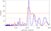 |
Fig. 3. Results of the LSP method in ZTF r-band (solid red) and g-band (solid blue) light curves. The vertical red line and blue line mark the positions of the corresponding peaks of the power, the dashed and solid orange lines respectively show the 3σ and 5σ significance level determined by false alarm probability. |
The WWZ method, based on wavelet analysis and vector projection, employs z-statistics for period extraction. It enhances the performance of traditional wavelet techniques for realistic data, particularly when the data are sparse and unevenly sampled. We employed the Python code from3 to calculate the WWZ power with frequency steps of 0.0001 in frequency range from 0.0025 to 0.1 day−1, and the results are illustrated in Figure 4. The periodicities of 221 ± 15 days in ZTF r-band and 220 ± 6 days in ZTF g-band light curves were identified by the WWZ method, and are consistent with those obtained from the LSP method, and the uncertainties were determined by the bootstrap method, as described above.
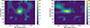 |
Fig. 4. Results of the WWZ method in ZTF r-band (left panel) and g-band (right panel) light curves of SDSS J1532. In each panel the horizontal red line represents the position of the corresponding periodicity. |
The presence of red noise in the optical band can significantly influence the detection of QPOs. Red noise has the potential to obscure genuine QPO signals, and can also mimic periodic variability through a few-cycle sinusoid-like modulation (Vaughan et al. 2016). Therefore, it is important to evaluate the likelihood of spurious QPO detections in light curves generated purely from stochastic processes such as the continuous autoregressive (CAR) or damped random walk (DRW) models with the basic parameters of the intrinsic variability amplitude σ and the intrinsic variability timescale τ. A comparison between a pure red noise (DRW) model and a DRW model with an additional sinusoidal component may not always provide a clear distinction regarding the presence of periodic variability. In practice, the DRW model alone can reproduce a sinusoidal-like signal reasonably well under realistic sampling conditions, suggesting that stochastic red noise may partially mimic or absorb a periodic component, while QPO signals in AGNs are generally not perfectly sinusoidal. In addition, Witt et al. (2022) showed that periodic signals become increasingly difficult to distinguish from red noise when the signal amplitude is small or comparable to the stochastic variability. Therefore, in this work we do not adopt a DRW + sinusoidal model to describe the light curve of SDSS J1532.
To this end, we generated 100 000 artificial light curves using the CAR process with the following parameters: a characteristic timescale of τ = 188 days, as determined by the publicly available JAVELIN code (Kozłowski et al. 2010; Zu et al. 2013) in the ZTF g-band light curve, and a long-term variance τσ2/2 = 0.085, consistent with the observed variance of the ZTF g-band light curve. Given the larger number of data points in the g-band, the synthetic light curves generated in this work adopted the same time sampling as the original ZTF g-band data. We then applied the following three criteria to identify potential false QPO detections among the simulated light curves: (1) The light curve must exhibit a strong periodic signal, with a LSP power greater than 5σ significance level and a detected period between 180 and 260 days. (2) The light curve must be well described by a model consisting of a sinusoidal function added to a sixth-degree polynomial trend, with a χ2/d.o.f. less than 8 (two times larger than that of the observed light curve) and a fitted period within the same range (180–260 days). (3) The sinusoidal amplitude in the fitted artificial light curves is greater than 0.06 after considering that the sinusoidal fit to the ZTF g-band light curve yields an amplitude of 0.12. Among the 100 000 CAR-generated light curves, there are 178 light curves that satisfy all three criteria. So the probability of detecting fake QPOs is 0.178% (corresponding to a confidence level higher than 3σ).
To assess the reliability of the periodicities determined by the WWZ and LSP methods, we employed the epoch-folding method to describe the light curves through a sinusoidal function. After subtracting the contributions of the six-degree polynomial function, the ZTF r-band and g-band light curves were folded, and the best-fitting periods were found to be 226 (χ2/d.o.f. = 4.89,d.o.f. = 236) and 225 days (χ2/d.o.f. = 7.07,d.o.f. = 283) for the ZTF r-band and g-band, respectively. Here the subtractions of the polynomial components can lead to more apparent folded results. It can be accepted that there is little difference in the best-fitting periods between the ZTF r-band and g-band light curves because the light curves in different bands are fitted independently and have slightly different sampling and noise properties. The best-fitting periods for CSS light curve is 223 days (χ2/d.o.f. = 3.54,d.o.f. = 61). Figure 5 shows best-fitting results by the epoch-folding method. The relatively large χ2/d.o.f. values reflect the presence of stochastic, red noise-like variability that is not captured by a simple sinusoidal model; therefore, the fits are used only to characterize the periodic modulation rather than to fully reproduce the detailed light curve structure. Moreover, each of the three folded light curves is also described by a one-degree polynomial, and the χ2/d.o.f. determined by the best-fitting results are 6.88, 8.51, and 4.63, respectively. Based on the F-test technique, a sinusoidal function is preferred to a one-degree polynomial with confidence level higher than 5σ.
 |
Fig. 5. Epoch-folding method results of ZTF 5 day binned r-band light curve with a 226 day periodicity (left panel), ZTF 5 day binned g-band light curve with a 225 day periodicity (middle panel) after subtracting the contributions of the six-degree polynomial function, and CSS 1 day binned light curve with a 223 day periodicity (right panel). In each panel, the solid and dashed purple lines show the best-fitting descriptions by sinusoidal function and their corresponding 1RMS scatters, respectively. |
Moreover, as discussed in VanderPlas (2018), the various observational patterns inevitably imprint on the power spectrum derived from the observed data. To confirm the reliability of the observed peak, we searched the Asteroid Terrestrial-impact Last Alert System (ATLAS; Tonry et al. 2018) c-band data of SDSS J1532, and present its light curve in the left panel of Figure 6. Given that the ATLAS light curve covers a similar time span to that of the ZTF, but has larger uncertainties, we applied the LSP method to the ATLAS c-band light curve solely for the purpose of testing periodicity, in order to eliminate the possibility of spurious signals arising from various observational patterns. As shown in the right panel of Figure 6, we find that the ATLAS c-band also exhibits a periodicity of approximately 214 days. The data used in this analysis were also obtained by subtracting a first-order polynomial function from the observed light curves. Thus, the periodicity of about 220 days for SDSS J1532 is not the result of the observational pattern.
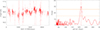 |
Fig. 6. ATLAS c-band light curve of SDSS J1532 (left panel) and the result of LSP method in the ATLAS c-band light curve (right panel). In the right panel, the vertical red line marks the position of the peak of the power, and the dashed and solid orange lines respectively show the 3σ and 5σ confidence levels determined by the false alarm probability. |
3. Main results and discussions
3.1. Spectroscopic features
As discussed in Xu & Komossa (2009), Zheng et al. (2024), objects with double-peaked profiles in all narrow emission lines could strengthen the presence of kiloparsec-scale dual AGN candidates. However, most objects exhibit double-peaked profiles only in [O III] (Zhou et al. 2004; Kim et al. 2020; Zheng et al. 2025), while those with prominent double peaks across all narrow emission lines are predominantly found in type 2 AGNs (Wang et al. 2009; Xu & Komossa 2009; Severgnini et al. 2021). Only a small number of type 1 AGNs display such profiles consistently in all narrow lines (Ge et al. 2012; Zheng et al. 2024). SDSS J1532 is a good candidate for a kiloparsec-scale dual AGN with double-peaked profiles in all of its narrow emission lines. In addition, NLR kinematics, such as a rotating disk-like NLR and AGN-driven outflow (Crenshaw et al. 2010; Barrows et al. 2013), are also discussed to explain the presence of DPNELs in SDSS J1532.
If it is assumed that the dual AGN scenario is responsible for the double-peaked profiles in all narrow lines of SDSS J1532, given the mean peak separation of Δυ ∼ 340 km/s, as shown in Table 1, then the physical separation between the two putative AGN cores can be simply estimated using a circular motion equation,  , where M1 and M2 denote the total mass of each core, r represents the intrinsic spatial distance between the two cores, and i and ϕ are the inclination angle of the rotation plane and the orientation angle, respectively. Since i and ϕ are not observationally constrained, we adopt the maximum projection factor (sin(i)cos(ϕ) = 1, corresponding to i = 90° and ϕ = 0°), which provides an upper limit on r.
During the dual AGN phase, each black hole is expected to retain the stellar component of its original host galaxy; we therefore use the corresponding total stellar masses M* as proxies for M1 and M2. The total stellar mass can be determined through the M*–σ* relation (stellar velocity dispersion) (Li et al. 2013; Zahid et al. 2016; Damjanov et al. 2022). Since the spectrum of SDSS J1532 lacks discernible spectroscopic features from the host galaxy, the most practical approach is to utilize the line width of narrow emission lines as a tracer of σ* (Nelson & Whittle 1996; Greene & Ho 2005a). Using the line widths of [O III] as proxies for σ*, the estimated M* values for the two putative cores are 1010.72 ± 0.30 M⊙ and 1010.69 ± 0.29 M⊙, respectively, with uncertainties arising from both the line width and the parameters of the M*–σ* relation. Further details about the calculation of M* can be found in Zheng et al. (2024). After treating M* as M1 and M2, the upper limit of r is estimated to be 3.14 ± 2.64 kpc. The inferred kiloparsec-scale separation is consistent with the expectations for dual AGNs, where the two narrow-line regions remain spatially distinct and can produce double-peaked narrow emission lines. Because the broad-line region emission from the two putative nuclei cannot be disentangled, separate virial black hole (BH) mass estimates for each component are not feasible. Therefore, the BH mass MBH can be calculated by the MBH − σ* relation, which is also applicable in dual cores (Gebhardt et al. 2000; Johansson et al. 2009; Sahu et al. 2019; Bennert et al. 2021). Based on the relation in Kormendy & Ho (2013) and the widths of [O III] as tracers of σ*, the values of MBH are 107.61 ± 0.20 M⊙ and 107.52 ± 0.20 M⊙.
In the rotating disk-like NLR scenario, the two sets of emission lines are illuminated by a single ionizing source, and there is expected to be a similar physical condition in the narrow-line region on both sides (Xu & Komossa 2009). Consequently, comparing the line ratios of the two components provides a useful diagnostic for testing the disk interpretation. Although projection effects may introduce differences in the observed line widths and fluxes, large discrepancies in intrinsic line ratios are generally not expected in a simple rotating disk. Based on the parameters listed in Table 1, the line flux ratios for the blueshifted component and the redshifted component exhibit similar values in most narrow emission lines, such as Hα/[O III] ratios, broadly consistent with the disk scenario. However, the Hα/[N II] ratios show a significant contrast, with values of 5.3 ± 0.9 and 2.5 ± 0.4 for the blueshifted and redshifted components, respectively. Moreover, according to the criterion in Smith et al. (2012), the similar line flux ratio of the blueshifted component to the redshifted component (0.75 ≤ Fb/Fr ≤ 1.25) often represents a rotating disk. Most of the line flux ratios in double-peaked profiles of SDSS J1532 are consistent with this criterion, but show large difference in [N II] and [S II]. Taken together, these results suggest that while some spectral properties are consistent with a rotating disk, the observed line ratio differences indicate that a simple disk model alone may not fully explain the double-peaked structure.
In the AGN-driven outflow scenario, a biconical outflow, moving toward and away from the observer, could naturally generate DPNELs. Due to extinction by dust in the galaxy and the outflow itself, the redshifted components would experience more obscuration, and then typically exhibit smaller line fluxes, compared to the blueshifted component (Liu et al. 2010). However, in SDSS J1532, the fluxes of the redshifted and blueshifted components are comparable within the measurement uncertainties for most narrow emission lines, and no systematic attenuation of the redshifted component is observed. This behavior is not clearly consistent with the simple expectations of a dust-obscured outflow scenario. Additionally, a strong outflow is expected to induce velocity stratification between lines originating closer to the core and lines at larger distances (Xu & Komossa 2009). However, as shown in Table 1, the peak separations Δυ between the blueshifted and redshifted components are consistent among all these narrow emission lines, showing no evidence for such stratification. So it disfavors the AGN-driven outflow scenario.
3.2. QPO properties
A periodicity of about 220 day is determined in ZTF r-band and g-band light curves when utilizing the LSP method, WWZ method, and epoch-folding method. To investigate the origins of the QPO signal observed in SDSS J1532, three models are discussed here: the BBH model, the disk precession model, and the jet precession model.
In the BBH scenario (Graham et al. 2015; Kovačević et al. 2019; Zhang 2023), it been proposed to explain long-standing QPOs with periodicities spanning from hundreds to thousands of days. According to the discussion in Eracleous et al. (2012), the space separation of the BBH system can be calculated as
 (1)
(1)
where M8 is the MBH in units of 108 M⊙. After considering the BH mass MBH range from 107.52 ± 0.20 M⊙ to 107.61 ± 0.20 M⊙ and the periodicity as about 220 day (P ∼ 0.6 yr), the space separation between the central BBH might be about 0.95–1.4 mpc.
In the disk precession scenario (Armstrong et al. 2013; Zhang 2023), the disk precesses relative to its local frame of reference as a result of the rotation of massive black hole. According to Eracleous et al. (1995), Storchi-Bergmann et al. (2003), the anticipated period of disk precession can be approximated as  , where R3 represents the distance of emission regions to the central BH in units of 103 Schwarzschild radii (RG = GMBH/c2). Then the expected R3 is about 0.061–0.095 (61–95 RG). Additionally, according to the results of Morgan et al. (2010), based on microlensing variability analyses of 11 gravitationally lensed quasars, the size of the near-ultraviolet (NUV) 2500 Å continuum emission region in SDSS J1532 is given by
  –88 RG. In the framework of the standard thin-disk model (Frank et al. 2002; Fausnaugh et al. 2016; Lasota 2022), the disk temperature decreases with increasing radius. As a result, NUV emission is expected to originate from the hotter inner regions of the accretion disk, while the optical emission is produced at relatively larger radii. However, the radii inferred above for the optical and NUV continua are comparable, indicating that the two bands originate from similar characteristic disk scales rather than from widely separated regions. Since the ZTF g-band emission originates from regions closer to the central engine, the disk precession model would predict a slightly shorter period in the g-band compared to that in the r-band. However, the periodicities derived from the aforementioned methods are generally consistent between the two bands. The results do not support the disk precession scenario as the origin of the periodic modulation.
In the jet precession scenario (Caproni et al. 2013; Bhatta 2018; Zhang et al. 2021), the brightness of a source varies as a result of the helical structure. However, despite being observed in the Faint Images of the Radio Sky at Twenty-cm (Becker et al. 1995; Helfand et al. 2015), SDSS J1532 does not exhibit any apparent radio emissions. Therefore, jet precession is not a better choice for the optical QPO in SDSS J1532.
3.3. Future applications
Although alternative interpretations cannot be ruled out with the current observational evidence, SDSS J1532 remains a good candidate for a triple black hole with a close BBH pair. The double-peaked profiles observed in all narrow emission lines suggest the presence of a dual AGN system on kiloparsec scales, with an estimated projected separation of ∼3 kpc. Such a separation would correspond to an orbital timescale of several gigayears, far exceeding the temporal coverage of the current photometric data, and therefore cannot be tested through light curve folding. In contrast, the QPO likely originates from a much more compact BBH system embedded within one of the nuclei, with an inferred separation of ∼1 mpc. Therefore, one of the nuclei in the dual AGN may itself host a close binary black hole. On subparsec scales, the NLRs are expected to merge into a common region, making split or broadened narrow lines unlikely, whereas the more compact broad-line regions may remain distinct. If both nuclei were type 1 AGNs, double-peaked broad emission lines would be expected. However, the absence of obvious double-peaked broad lines in SDSS J1532 suggests that only one of the compact nuclei likely contributes broad-line emission. If feasible, future observations with higher spatial or temporal resolution could help confirm or reject these scenarios by providing stronger constraints on the nature of the multiple components.
Evidence for triple black holes can not only validate the hierarchical merger paradigm, but will also significantly advance our understanding of galaxy formation and fundamental physics. Furthermore, the presence of triple black holes offers a unique opportunity to study the dynamics of three-body interactions within the framework of general relativity (Merritt 2006). Theoretical predictions indicate that hierarchical systems of closely spaced triple black holes potentially generate intense bursts of gravitational waves (Iwasawa et al. 2006; Lousto & Zlochower 2008). These gravitational waves hold the potential for detection by low-frequency gravitational wave experiments in the future (Amaro-Seoane et al. 2010; Caprini & Figueroa 2018; Caprini et al. 2020; Auclair et al. 2023).
4. Summary and conclusions
The main summary and our conclusions are as follows:
-
SDSS J1532 shows the properties of DPNELs in all narrow emission lines with peak separations of about 340 km/s, which might be produced by a dual AGN on kiloparsec-scale.
-
The similar line flux ratios of the blueshifted and redshifted components in most of the DPNELs are broadly consistent with a disk scenario, while the significantly different Hα/[N II] ratios suggest that a simple rotating disk model may not fully explain the observed double-peaked structure.
-
The similarity of line fluxes in the blueshifted and redshifted components and the similarity of peak separations in different double-peaked features disfavor the AGN-driven outflow model.
-
SDSS J1532 shows an optical quasiperiodic oscillation with a period of ∼0.6 yr, corresponding to ∼10.5 cycles in the ZTF light curve, while the CSS light curve independently covers ∼13.5 cycles.
-
Since the optical emission region estimated by disk precession is similar to NUV emission regions, and there is no apparent radio emission in SDSS J1532, it is opposite to the disk precession and jet precession models. In the BBH model scenario, the estimated distance is about 1 mpc between the two central BHs.
-
Although alternative interpretations cannot be ruled out with the current observational evidence, the observed double-peaked narrow emission lines and the optical quasiperiodic oscillation are broadly consistent with a triple black hole scenario, in which the kiloparsec-scale double-peaked features may arise from a dual AGN and the optical quasiperiodic modulation may be associated with a subparsec binary black hole. If SDSS J1532 is confirmed as a triple black hole system with a close BBH, it would signify a pivotal moment in the evolution of galaxy mergers.
Acknowledgments
We gratefully acknowledge the anonymous referee for giving us constructive comments and suggestions to greatly improve our paper. We thank Paola Severgnini and Fabio Rigamonti (INAF–Brera Astronomical Observatory) and Cristian Vignali (University of Bologna) for their valuable comments and helpful suggestions that greatly improved this work. This work is supported by the National Natural Science Foundation of China (Nos. 12273013, 12173020, 12373014). We have made use of the data from SDSS DR16. The SDSS DR16 website is (http://skyserver.sdss.org/dr16/en/home.aspx). The MPFIT website is (http://cow.physics.wisc.edu/~craigm/idl/idl.html). The ZTF data can be obtained in the web site (https://irsa.ipac.caltech.edu/frontpage/). The CSS web site is (http://nesssi.cacr.caltech.edu/DataRelease/). The ATLAS web site is (https://fallingstar-data.com/forcedphot/).
References
- Ahumada, R., Allende Prieto, C., Almeida, A., et al. 2020, ApJS, 249, 3 [NASA ADS] [CrossRef] [Google Scholar]
- Amaro-Seoane, P., Sesana, A., Hoffman, L., et al. 2010, MNRAS, 402, 2308 [NASA ADS] [CrossRef] [Google Scholar]
- Armstrong, E., Patterson, J., Michelsen, E., et al. 2013, MNRAS, 435, 707 [NASA ADS] [CrossRef] [Google Scholar]
- Auclair, P., Bacon, D., Baker, T., et al. 2023, Liv. Rev. Rel., 26, 5 [Google Scholar]
- Banerjee, A., Negi, V., Joshi, R., et al. 2023, MNRAS, 526, 5172 [Google Scholar]
- Barrows, R. S., Sandberg Lacy, C. H., Kennefick, J., et al. 2013, ApJ, 769, 95 [NASA ADS] [CrossRef] [Google Scholar]
- Barth, A. J., Bentz, M. C., Greene, J. E., et al. 2008, ApJ, 683, 119 [Google Scholar]
- Becker, R. H., White, R. L., & Helfand, D. J. 1995, ApJ, 450, 559 [Google Scholar]
- Begelman, M. C., Blandford, R. D., & Rees, M. J. 1980, Nature, 287, 307 [Google Scholar]
- Bellm, E. C., Kulkarni, S. R., Graham, M. J., et al. 2019, PASP, 131, 018002 [Google Scholar]
- Bennert, V. N., Treu, T., Ding, X., et al. 2021, ApJ, 921, 36 [NASA ADS] [CrossRef] [Google Scholar]
- Bhatta, G. 2018, Galaxies, 6, 136 [Google Scholar]
- Bhatta, G. 2021, ApJ, 923, 7 [CrossRef] [Google Scholar]
- Britzen, S., Fendt, C., Witzel, G., et al. 2020, IAU Symp., 342, 250 [Google Scholar]
- Caprini, C., & Figueroa, D. G. 2018, Class. Quant. Grav., 35, 3001 [Google Scholar]
- Caprini, C., Chala, M., Dorsch, G. C., et al. 2020, JCAP, 03, 024 [CrossRef] [Google Scholar]
- Caproni, A., Abraham, Z., & Monteiro, H. 2013, MNRAS, 428, 280 [NASA ADS] [CrossRef] [Google Scholar]
- Chen, Y., Yi, T., & Chen, J. 2024, NewA, 108, 02186 [Google Scholar]
- Comerford, J. M., Gerke, B. F., Stern, D., et al. 2012, ApJ, 753, 42 [Google Scholar]
- Comerford, J. M., Nevin, R., Stemo, A., et al. 2018, ApJ, 867, 66 [NASA ADS] [CrossRef] [Google Scholar]
- Crenshaw, D. M., Schmitt, H. R., Kraemer, S. B., et al. 2010, ApJ, 708, 419 [Google Scholar]
- Damjanov, I., Sohn, J., Utsumi, Y., et al. 2022, ApJ, 929, 61 [NASA ADS] [CrossRef] [Google Scholar]
- De Rosa, A., Vignali, C., Severgnini, P., et al. 2023, MNRAS, 519, 5149 [NASA ADS] [CrossRef] [Google Scholar]
- Deane, R. P., Paragi, Z., Jarvis, M. J., et al. 2014, Nature, 511, 57 [Google Scholar]
- Dekany, R., Smith, R. M., Riddle, R., et al. 2020, PASP, 132, 038001 [NASA ADS] [CrossRef] [Google Scholar]
- Dexter, J., & Agol, E. 2011, ApJ, 727, 24 [NASA ADS] [CrossRef] [Google Scholar]
- Djorgovski, S. G., Courbin, F., Meylan, G., et al. 2007, ApJ, 662, 1 [Google Scholar]
- Drake, A. J., Djorgovski, S. G., Mahabal, A., et al. 2009, ApJ, 696, 870 [Google Scholar]
- Eracleous, M., Livio, M., Halpern, J. P., & Storchi-Bergmann, T. 1995, ApJ, 438, 610 [NASA ADS] [CrossRef] [Google Scholar]
- Eracleous, M., Boroson, T. A., Halpern, J. P., & Liu, J. 2012, ApJS, 201, 23 [Google Scholar]
- Farina, E. P., Montuori, C., Decarli, R., et al. 2013, MNRAS, 431, 1019 [NASA ADS] [CrossRef] [Google Scholar]
- Fausnaugh, M. M., Denney, K. D., Barth, A. J., et al. 2016, ApJ, 821, 5 [NASA ADS] [CrossRef] [Google Scholar]
- Foord, A., Gültekin, K., Runnoe, J. C., et al. 2021a, ApJ, 907, 71 [NASA ADS] [CrossRef] [Google Scholar]
- Foord, A., Gültekin, K., Runnoe, J. C., et al. 2021b, ApJ, 907, 72 [NASA ADS] [CrossRef] [Google Scholar]
- Foreman-Mackey, D., Hogg, D. W., Lang, D., et al. 2013, PASP, 125, 306 [NASA ADS] [CrossRef] [Google Scholar]
- Foster, G. 1996, AJ, 112, 1709 [NASA ADS] [CrossRef] [Google Scholar]
- Foustoul, V., Webb, N. A., Mignon-Risse, R., et al. 2025, A&A, 699, A55 [NASA ADS] [CrossRef] [EDP Sciences] [Google Scholar]
- Frank, J., King, A., & Raine, D. J. 2002, Accretion Power in Astrophysics, 3rd edn. (Cambridge University Press) [Google Scholar]
- Fu, H., Yan, L., Myers, A. D., et al. 2012, ApJ, 745, 67 [Google Scholar]
- Fukumura, K., Kazanas, D., & Stephenson, G. 2009, ApJ, 695, 1199 [Google Scholar]
- Ge, J. Q., Hu, C., Wang, J. M., et al. 2012, ApJS, 201, 31 [Google Scholar]
- Gebhardt, K., Bender, R., Bower, G., et al. 2000, ApJ, 539, 13 [Google Scholar]
- Graham, M. J., Djorgovski, S. G., Stern, D., et al. 2015, MNRAS, 453, 1562 [Google Scholar]
- Graham, M. J., Kulkarni, S. R., Bellm, E. C., et al. 2019, PASP, 131, 078001 [Google Scholar]
- Greene, J. E., & Ho, L. C. 2005a, ApJ, 627, 721 [NASA ADS] [CrossRef] [Google Scholar]
- Helfand, D. J., White, R. L., & Becker, R. H. 2015, ApJ, 801, 26 [NASA ADS] [CrossRef] [Google Scholar]
- Hopkins, P. F., Hernquist, L., Cox, T. J., et al. 2005, ApJ, 630, 705 [NASA ADS] [CrossRef] [Google Scholar]
- Huijse, P., Davelaar, J., De Ridder, J., Jannsen, N., & Aerts, C. 2025, ArXiv e-prints [arXiv:2505.16884] [Google Scholar]
- Iwasawa, M., Funato, Y., Makino, J., et al. 2006, ApJ, 651, 1059 [Google Scholar]
- Johansson, P. H., Naab, T., & Burkert, A. 2009, ApJ, 690, 802 [NASA ADS] [CrossRef] [Google Scholar]
- Kalfountzou, E., Santos Lleo, M., & Trichas, M. 2017, ApJ, 851, 15 [CrossRef] [Google Scholar]
- Kelly, B. C., Bechtold, J., & Siemiginowska, A. 2009, ApJ, 698, 895 [Google Scholar]
- Kim, D. C., Yoon, I., & Evans, A. S. 2020, ApJ, 904, 23 [Google Scholar]
- Kollatschny, W., Weilbacher, P. M., Ochmann, M. W., et al. 2020, A&A, 633, A79 [EDP Sciences] [Google Scholar]
- Kormendy, J., & Ho, L. C. 2013, ARA&A, 51, 511 [Google Scholar]
- Kovačević, A. B., Popović, L., Simić, S., et al. 2019, ApJ, 871, 32 [Google Scholar]
- Kozłowski, S., Kochanek, C. S., Udalski, A., et al. 2010, ApJ, 708, 927 [CrossRef] [Google Scholar]
- Lasota, J. P. 2022, in Active Galactic Nuclei, ed. F. Combes, 101 [Google Scholar]
- Law, N. M., Kulkarni, S. R., Dekany, R. G., et al. 2009, PASP, 121, 1395 [NASA ADS] [CrossRef] [Google Scholar]
- Li, C., Wang, L., & Jing, Y. P. 2013, ApJ, 762, 7 [Google Scholar]
- Li, X. P., Cai, Y., Yang, H. T., et al. 2021, MNRAS, 506, 1540 [Google Scholar]
- Li, X. P., Yang, H. Y., Cai, Y., et al. 2023, ApJ, 943, 157 [Google Scholar]
- Liu, X., Shen, Y., & Strauss, M. A. 2010, ApJ, 708, 427 [Google Scholar]
- Liu, X., Shen, Y., & Strauss, M. A. 2011, ApJ, 736, 7 [NASA ADS] [CrossRef] [Google Scholar]
- Liu, X., Civano, F., Shen, Y., et al. 2013, ApJ, 762, 110 [NASA ADS] [CrossRef] [Google Scholar]
- Liu, X., Lazio, T. J. W., Shen, Y., et al. 2018, ApJ, 854, 169 [Google Scholar]
- Lomb, N. R. 1976, Ap&SS, 39, 447 [Google Scholar]
- Lousto, C. O., & Zlochower, Y. 2008, Phys. Rev. D, 77, 4034 [Google Scholar]
- MacLeod, C. L., Ivezić, Ž., Kochanek, C. S., et al. 2010, ApJ, 721, 1014 [Google Scholar]
- Makridakis, S., Wheelwright, S. C., & Hyndman, R. J. 1997, Forecasting Methods and Applications (John Wiley& Sons) [Google Scholar]
- Markwardt, C. B. 2009, ASP Conf. Ser., 411, 251 [Google Scholar]
- Merritt, D. 2006, Rep. Prog. Phys., 69, 2513 [Google Scholar]
- Millon, M., Dalang, C., Lemon, C., et al. 2022, A&A, 668, A77 [NASA ADS] [CrossRef] [EDP Sciences] [Google Scholar]
- Morgan, C. W., Kochanek, C. S., Morgan, N. D., et al. 2010, ApJ, 712, 1129 [NASA ADS] [CrossRef] [Google Scholar]
- Nelson, C. H., & Whittle, M. 1996, ApJ, 465, 96 [NASA ADS] [CrossRef] [Google Scholar]
- Pandya, V., Zhang, H., Huertas-Company, M., et al. 2024, ApJ, 963, 54 [NASA ADS] [CrossRef] [Google Scholar]
- Vanden Berk, D. E., Richards, G. T., Bauer, A., et al. 2001, AJ, 122, 549 [Google Scholar]
- Wrobel, J. M., Walker, R. C., & Fu, H. 2014, ApJ, 792, 8 [NASA ADS] [CrossRef] [Google Scholar]
- Peng, S., Li, Z., Liu, X., et al. 2022, ApJ, 934, 89 [Google Scholar]
- Peterson, B. M., Ferrarese, L., Gilbert, K. M., et al. 2004, ApJ, 613, 682 [Google Scholar]
- Pfeifle, R. W., Satyapal, S., Manzano-King, C., et al. 2019, ApJ, 883, 167 [Google Scholar]
- Rau, A., Kulkarni, S. R., Law, N. M., et al. 2009, PASP, 121, 1334 [NASA ADS] [CrossRef] [Google Scholar]
- Sahu, N., Graham, A. W., & Davis, B. L. 2019, ApJ, 887, 10 [CrossRef] [Google Scholar]
- Sarkar, A., Kushwaha, P., & Gupta, A. C. 2020, A&A, 642, A129 [NASA ADS] [CrossRef] [EDP Sciences] [Google Scholar]
- Storey, P. J., & Zeippen, C. J. 2000, MNRAS, 312, 813 [NASA ADS] [CrossRef] [Google Scholar]
- Schulz, M., & Mudelsee, M. 2002, Comput. Geosci., 28, 421 [NASA ADS] [CrossRef] [Google Scholar]
- Serafinelli, R., Severgnini, P., Braito, V., et al. 2020, ApJ, 902, 10 [Google Scholar]
- Severgnini, P., Cicone, C., Della Ceca, R., et al. 2018, MNRAS, 479, 3804 [Google Scholar]
- Severgnini, P., Braito, V., Cicone, C., et al. 2021, A&A, 646, A153 [NASA ADS] [CrossRef] [EDP Sciences] [Google Scholar]
- Scargle, J. D. 1982, ApJ, 263, 835 [Google Scholar]
- Schawinski, K., Urry, M., Treister, E., et al. 2011, ApJ, 743, 37 [CrossRef] [Google Scholar]
- Schutte, Z., Reines, A. E., & Greene, J. E. 2019, ApJ, 887, 245 [NASA ADS] [CrossRef] [Google Scholar]
- Shen, Y., Richards, G. T., Strauss, M., et al. 2011, ApJS, 194, 45 [NASA ADS] [CrossRef] [Google Scholar]
- Shen, Y., Hwang, H., Zakamska, N., et al. 2019, ApJ, 885, 4 [Google Scholar]
- Silk, J., & Rees, M. J. 1998, A&A, 331, L1 [NASA ADS] [Google Scholar]
- Smith, K. L., Shields, G. A., Bonning, E. W., et al. 2010, ApJ, 716, 866 [Google Scholar]
- Smith, K. L., Shields, G. A., Salviander, S., et al. 2012, ApJ, 752, 63 [Google Scholar]
- Storchi-Bergmann, T., Nemmen da Silva, R., Eracleous, M., et al. 2003, ApJ, 598, 956 [NASA ADS] [CrossRef] [Google Scholar]
- Templeton, M. 2004, JAAVSO, 32, 41 [NASA ADS] [Google Scholar]
- Tonry, J. L., Denneau, L., Heinze, A. N., et al. 2018, PASP, 130, 4505 [Google Scholar]
- Toomre, A., & Toomre, J. 1972, ApJ, 178, 623 [Google Scholar]
- Valtonen, M. J. 1996, MNRAS, 278, 186 [NASA ADS] [CrossRef] [Google Scholar]
- VanderPlas, J. T. 2018, ApJS, 236, 16 [Google Scholar]
- Vaughan, S., Uttley, P., Markowitz, A. G., et al. 2016, MNRAS, 461, 3145 [Google Scholar]
- Vestergaard, M. 2002, ApJ, 571, 733 [NASA ADS] [CrossRef] [Google Scholar]
- Wang, J. M., Chen, Y. M., Hu, C., et al. 2009, ApJ, 705, 76 [Google Scholar]
- Wang, G. G., Cai, J. T., & Fan, J. H. 2022, ApJ, 929, 130 [NASA ADS] [CrossRef] [Google Scholar]
- Witt, C. A., Charisi, M., Taylor, S. R., et al. 2022, ApJ, 936, 89 [NASA ADS] [CrossRef] [Google Scholar]
- Xu, D. W., & Komossa, S. 2009, ApJ, 705, 20 [Google Scholar]
- Yang, J., Cao, G., Zhou, B., et al. 2021, PASP, 133, 4101 [Google Scholar]
- Zahid, H. J., Geller, M. J., Fabricant, D. G., et al. 2016, ApJ, 832, 203 [NASA ADS] [CrossRef] [Google Scholar]
- Zhang, H. Y., Yan, D. H., & Zhang, P. F. 2021, ApJ, 919, 58 [NASA ADS] [CrossRef] [Google Scholar]
- Zhang, X. G. 2023, MNRAS, 526, 1588 [NASA ADS] [CrossRef] [Google Scholar]
- Zheng, Q., Liu, S., Zhang, X. G., et al. 2023, ApJ, 944, 4 [Google Scholar]
- Zheng, Q., Zhang, X. G., Yuan, Q. R., et al. 2024, MNRAS, 531, 76 [Google Scholar]
- Zheng, Q., Ma, Y. S., Zhang, X. G., et al. 2025, ApJS, 277, 49 [Google Scholar]
- Zhou, H. Y., Wang, T. G., Zhang, X. G., et al. 2004, ApJ, 604, 33 [Google Scholar]
- Zu, Y., Kochanek, C. S., Kozłowski, S., et al. 2013, ApJ, 765, 106 [NASA ADS] [CrossRef] [Google Scholar]
All Tables
All Figures
|
Fig. 1. Rest-frame optical spectrum of SDSS J1532 (top left panel) and best-fitting results of SDSS J1532 with rest-frame spectrum from 3850 Å to 4450 Å (top right panel), from 4750 Å to 5050 Å (bottom left panel) and from 6400 Å to 6800 Å (bottom right panel). In the top subpanels the solid dark green lines show the line spectra; the dashed blue and red lines represent the blueshifted and redshifted components of the narrow Hα, Hβ, Hγ, Hδ, He I, [Ne III], [O III], [N II], and [S II] doublets; the solid blue lines represent the extended components of the [O III] emission lines; the solid green lines represent the broad Hα, Hβ, and Hγ emission lines with the corresponding parameters of the central wavelength (Å), line width σ (Å), and line flux (10−17 erg/s/cm2) listed in the first two lines of the panels; the dashed cyan lines show the continuum emissions |
| In the text | |
|
Fig. 2. Observed optical light curves of SDSS J1532 directly downloaded from the survey archives of the CSS (v-band) and ZTF (g-band, r-band, i-band). The solid and dashed lines show the best-fitting results and their corresponding 1RMS scatter bands, respectively. The dotted lines represent the results of the polynomial function. |
| In the text | |
|
Fig. 3. Results of the LSP method in ZTF r-band (solid red) and g-band (solid blue) light curves. The vertical red line and blue line mark the positions of the corresponding peaks of the power, the dashed and solid orange lines respectively show the 3σ and 5σ significance level determined by false alarm probability. |
| In the text | |
|
Fig. 4. Results of the WWZ method in ZTF r-band (left panel) and g-band (right panel) light curves of SDSS J1532. In each panel the horizontal red line represents the position of the corresponding periodicity. |
| In the text | |
|
Fig. 5. Epoch-folding method results of ZTF 5 day binned r-band light curve with a 226 day periodicity (left panel), ZTF 5 day binned g-band light curve with a 225 day periodicity (middle panel) after subtracting the contributions of the six-degree polynomial function, and CSS 1 day binned light curve with a 223 day periodicity (right panel). In each panel, the solid and dashed purple lines show the best-fitting descriptions by sinusoidal function and their corresponding 1RMS scatters, respectively. |
| In the text | |
|
Fig. 6. ATLAS c-band light curve of SDSS J1532 (left panel) and the result of LSP method in the ATLAS c-band light curve (right panel). In the right panel, the vertical red line marks the position of the peak of the power, and the dashed and solid orange lines respectively show the 3σ and 5σ confidence levels determined by the false alarm probability. |
| In the text | |
Current usage metrics show cumulative count of Article Views (full-text article views including HTML views, PDF and ePub downloads, according to the available data) and Abstracts Views on Vision4Press platform.
Data correspond to usage on the plateform after 2015. The current usage metrics is available 48-96 hours after online publication and is updated daily on week days.
Initial download of the metrics may take a while.