


| Issue |
A&A
Volume 710, June 2026
|
|
|---|---|---|
| Article Number | A131 | |
| Number of page(s) | 14 | |
| Section | Numerical methods and codes | |
| DOI | https://doi.org/10.1051/0004-6361/202557715 | |
| Published online | 05 June 2026 | |
BGRem: A background noise remover for astronomical images based on a diffusion model
1
Institute for Mathematics, Astrophysics and Particle Physics (IMAPP), Radboud University Nijmegen,
Heyendaalseweg 135,
6525
AJ
Nijmegen,
The Netherlands
2
Nikhef,
Science Park 105,
1098
XG
Amsterdam,
The Netherlands
3
Department of Physics, University of Oxford,
Denys Wilkinson Building, Keble Road,
Oxford
OX1 3RH,
UK
4
University of Nova Gorica, Centre for Astrophysics and Cosmology,
Vipavska 11c,
Ajdovščina,
Slovenia
5
Instituto de Física Corpuscular (IFIC), CSIC-UV,
Spain
6
Department of Astronomy and Inter-University Institute for Data Intensive Astronomy, University of Cape Town,
Private Bag X3,
Rondebosch
7701,
South Africa
7
South African Astronomical Observatory,
PO Box 9, Observatory,
Cape Town
7935,
South Africa
★ Corresponding authors: This email address is being protected from spambots. You need JavaScript enabled to view it.
; This email address is being protected from spambots. You need JavaScript enabled to view it.
Received:
16
October
2025
Accepted:
28
March
2026
Abstract
Context. Astronomical imaging aims to maximize signal capture while minimizing noise. It is difficult and expensive to enhance the signal-to-noise ratio directly on detectors, which has led to extensive research into advanced post-processing techniques.
Aims. Removing background noise from images is a valuable preprocessing step for catalog-building tasks. We introduce BGRem, a machine-learning (ML)-based tool to remove background noise from astronomical images. Our aim is to improve image quality and enhance the performance of the subsequent analysis pipeline, from detecting faint sources to performing source characterization tasks.
Methods. The BGRem tool uses a diffusion-based model with an attention U-Net as backbone, trained on simulated images for optical and gamma (γ)-ray data from the MeerLICHT and Fermi-LAT telescopes. The tool learns to denoise astronomical images in a supervised manner over several diffusion steps. We performed preprocessing and postprocessing techniques, including normalization and median subtraction, on these images to make them suitable for the analysis pipeline.
Results. We compared the performance of BGRem with SourceExtractor (SExtractor), a widely used tool for cataloging astronomical sources. The number of true positive sources using SExtractor increased by about 7% for MeerLICHT data when we used BGRem as a preprocessing step. We also show the generalizability of BGRem by testing it with optical images from different telescopes and on simulated γ-ray data representative of the Fermi-LAT telescope. In both cases, BGRem improves the source detection efficiency.
Conclusions. The BGRem tool improves the source detection accuracy of traditional pixel-based methods by removing complex background noise. Using zero-shot approach, BGRem generalizes well to a wide range of optical images. The successful application of BGRem to simulated γ-ray images, alongside optical data, demonstrates its adaptability to distinct noise characteristics and observational domains. This cross-wavelength performance highlights its potential as a general-purpose background removal framework for multiwavelength astronomical surveys.
Key words: methods: data analysis / techniques: image processing
© The Authors 2026
 Open Access article, published by EDP Sciences, under the terms of the Creative Commons Attribution License (https://creativecommons.org/licenses/by/4.0), which permits unrestricted use, distribution, and reproduction in any medium, provided the original work is properly cited.
This article is published in open access under the Subscribe to Open model. This email address is being protected from spambots. You need JavaScript enabled to view it. to support open access publication.
1 Introduction
Astronomical imaging is fundamentally challenged by the need to maximize signal capture while minimizing noise interference. Achieving a high signal-to-noise ratio (S/N) is crucial for ensuring the reliability and accuracy of scientific analyses derived from these images. However, enhancing the S/N directly on the detector is both technically and financially difficult. Although shot noise (Poisson noise), related to random fluctuations in the photon counts, is the common form of noise, instrumental noises such as readout noise and dark current noise also affect image quality. While increasing the exposure time can increase the signal, noise also increases. Stacking images (referred to as coaddition) increases the S/N and depth of the images. However, these images may be taken under different atmospheric conditions (transparency) and background levels, and may be affected by variations in instrumental optical quality as quantified by the point spread function(PSF) across different parts of the sky. Methods to improve the process of addition are an active area of research (Zackay & Ofek 2017a,b), as they play a significant role in ongoing surveys such as the Zwicky Transient Facility (ZTF) (Bellm et al. 2018), and in the near future, the Vera C. Rubin Observatory’s Legacy Survey of Space and Time (LSST) (Ivezić et al. 2019). Several traditional methods, such as bilateral filtering, wavelets-based methods, nonlocal means, and block matching (for a comprehensive review, see Roscani et al. 2020), are often used as processing steps for astronomical image enhancement tasks.
Over the last decade, several machine learning (ML)-based algorithms, specifically deep neural network (DNN)-inspired techniques, have been used for image denoising tasks (for a review of modern techniques, see Tian et al. 2020). Machine learning (ML) models are strongly dependent on the quality and characteristics of their training data. Many models are trained on simulated data, where the ground truth is controlled and assumptions about background noise are predefined. However, generalizing these models to real data, which always includes noise, remains a significant challenge. For astronomical images, a deep convolutional autoencoder network effectively denoises radio images and detects faint sources (Gheller & Vazza 2021). For optical images from the Hubble Space Telescope, a U-Net-based (Ronneberger et al. 2015) denoising network, “Astro U-Net” (Vojtekova et al. 2020) produces images with noise characteristics similar to those obtained with twice the exposure. Recently, a DNN-based image restoration algorithm with active learning has been tested on large-scale sky surveys (Jia et al. 2023) and minimizes the impact of noise and PSFs.
Beyond image denoising, Wolf et al. (2024) show that their convolutional autoencoder neural network increases sensitivity for exoplanet direct imaging by up to 2.6 times compared to conventional methods. Ehlert et al. (2022) developed a probabilistic method to remove background from low-signal X-ray and γ-ray event list data from observatories. They show that their method, which accounts for random Poisson fluctuations, yields more significant galaxy cluster detections than standard background subtraction. Acciarri et al. (2021) used a UResNet (U-net with residual-net as backbone) to denoise neutrino detections, employing segmentation to differentiate between neutrino interaction pixels and background pixels and showing promising results on simulated data. In their search for a rare decay in a particle detector experiment, Tung et al. (2024) successfully integrate a convolutional neural network with the statistical technique of pulse shape discrimination. This approach enabled them to suppress neutron background events by a factor of 5.6 · 105, while maintaining a photon signal acceptance rate of ~70%.
In this work, we present BGRem, an ML–based tool, built on the Gaussian diffusion framework (Sohl-Dickstein et al. 2015; Ho et al. 2020; Song et al. 2020), to remove background noise from astronomical images. Diffusion models form a category of generative models and are effective for text-to-image generation, image inpainting, super-resolution, and other applications (for a review of diffusion models in vision, see Croitoru et al. 2023). In BGRem, we draw on diffusion models for denoising tasks within a supervised ML scheme with an attention U-Net (Oktay et al. 2018) as the backbone. To quantify and compare our results, we used the background subtraction method in Source-Extractor (SExtractor) (Bertin & Arnouts 1996) for astronomical images. The SExtractor automatically detects sources in astronomical images, with background subtraction being a key preprocessing step. Our experiments show that BGRem removes background noise for optical images from different telescopes as well as from γ-ray simulated data, with high accuracy and within a reasonable computation time compared to SExtractor.
This study extends the end-to-end ML-based pipeline, AutoSourceID (ASID) (Panes et al. 2021), which enhances and complements traditional pixel-based methods. We previously developed astrophysical source detection and localization pipelines for optical (Stoppa et al. 2022) and gamma-ray sources (Panes et al. 2021; van den Oetelaar et al. 2021), which improve pixel-based and likelihood-based methods. The pipeline components ASID-FE (Stoppa et al. 2023b) and ASID-C (Stoppa et al. 2023a) were developed for the characterization of detected sources using DNNs, such as flux estimation and star-galaxy classification. We show that BGRem can be used as a background removal step prior to applying the source detection and localization pipeline, thus improving the catalog-building task. All code used to produce the results shown here is publicly available on GitHub1.
In Sect. 2, we describe the training data and preprocessing methods. Section 3 discusses the model, including postprocessing methods. In Sect. 4, we present the results and evaluate the performance of BGRem on test datasets and real-world applications. Finally, Sect. 5 provides a summary of our findings and explores future research directions.
2 Training data preparation
The training data consisted of five simulated full-field images from the MeerLICHT telescope (Groot et al. 2024), an optical telescope at the University of Cape Town2. We simulated three additional images and used these as test data. For the simulation, we used the GalSim (Rowe et al. 2015) simulation software with the corresponding background components: (a) a spatially varying sky background, (b) detector-level effects including Gaussian read noise and dark current, and (c) Poisson noise fluctuations from both the sky and the dark current.
Simulations are advantageous for training BGRem since they provide ground truth images, which are source-only images without background noise. In contrast, such ground truth is fundamentally inaccessible from real observations; background-reduced images can be generated using a specific model or estimation algorithm, but these should not be considered ground truth for training an ML algorithm. Simulated data enable controlled supervised training but may not fully capture the complexity of the real observational artifacts. This limitation may affect model generalization and data interpretation, as previously shown for γ-ray data (Caron et al. 2023). In Sect. 4, we discuss the application and performance of BGRem on real data.
Similar to the MeerLICHT data, the simulated images have a shape of 10 560 × 10 560 pixels, which is too large and memory-consuming as input to a DNN for processing. We therefore divided them into 256 × 256 pixel sub-images, resulting in a total of 8405 images. We used 10% of these images as test data, leaving approximately 7500 images for training. To ensure the quality of the training data, we excluded images whose maximum pixel value was below 500. This threshold, a hyperparameter of the training process, primarily affects the training time and the performance of the model on brighter sources. We chose this threshold to maximize the amount of training data used while removing the images without any bright sources.
Before an image is fed into the model, it undergoes two preprocessing steps. First, we subtract the median pixel value. Since most of the image consists of background noise, the median pixel value provides an estimate of the background. This subtraction centers the noise around zero. This approach works only if the background is flat across the entire image, which is generally not the case. Therefore, an alternative method divides the image into smaller regions and applies the same procedure for each smaller image individually. The second step is normalization, which ensures that the pixel values fall within a range similar to the training data. This normalization factor can be set manually or estimated by BGRem. It is crucial that the input background noise has the same spread as the training data. This allows the model to recognize the noise in every image.
We used simulated gamma-ray (γ-ray) sky images to examine whether BGRem can be extended to wavelengths beyond the optical regime and to different background conditions. We used the procedure described in Panes et al. (2021) to generate simulated γ-ray sky maps for Fermi-Large Area Telescope (LAT) (Atwood et al. 2009) observation in the 1–2 GeV range. The simulated data are based on ten years of LAT observations and include the source properties of two of the most common source classes: active galactic nuclei (AGNs) and pulsars (PSRs). One of the main challenges in analyzing the γ-ray sky to detect and characterize these sources is the presence of interstellar emission (IEM; Acero et al. 2016; Abdollahi et al. 2020), which results from the interaction of energetic cosmic rays with the interstellar medium. Specifically, regions close to the Galactic plane (|b| < 20°), where the IEM contribution is significant, can result in spurious source detections and can also hide faint source populations. To test the possibility of removing this IEM with BGRem, we used the latest Fermi-LAT background model3 (Abdollahi et al. 2020) to generate γ-ray sky patches including point sources and the IEM. We used 12 000 patches of size 64 × 64, distributed randomly over the whole sky, to train BGRem to remove this IEM component and to evaluated its performance using 600 patches. These images represent photon counts in an effectively infinite-statistics scenario. For the 1–2 GeV energy bin, considering the LAT PSF, the pixel resolution is ~0.2° (deg). We tested BGRem on 1–2 GeV data as a proof-of-concept study, motivated by practical considerations. In this range, the LAT PSF is relatively narrow (~0.2°) compared to lower energies, while photon statistics remain substantially higher than at higher energy bins (>2 GeV), where source counts are negligible. This energy band therefore provides a well-balanced regime that avoids the effects of poor PSF and low statistics. To apply BGRem at a different energy range, a thorough hyperparameter search must be performed during training; however, the current framework serves as a starting point.
3 Model description: BGRem framework
The working engine behind BGRem is inspired by diffusion models. Standard diffusion model training starts with a clean image and iteratively adds noise during the forward process through a Markov chain until the image becomes pure Gaussian noise with zero mean and unit variance (Sohl-Dickstein et al. 2015; Ho et al. 2020). The goal of the reverse process is to learn the incremental iterative transformation starting from Gaussian noise to produce a coherent image in an unsupervised manner.
The BGRem framework uses astronomical images as input, which consist of ground-truth images (astrophysical sources only) with scaled noise added, and can be expressed as
![Mathematical equation: $\[x_t=y+\sigma_t \cdot x,\]$](/articles/aa/full_html/2026/06/aa57715-25/aa57715-25-eq1.png) (1)
(1)
where xt denotes the noisy image at diffusion step t, y is the clean source-only image, σt is the noise scale, and x is the background noise. This can be viewed as adding a portion of the background noise (σt · x) to the clean image, where we sample a random t (t ∈ [0, 1] ~ Uniform (0, 1)) from a uniform distribution. This sampled time is mapped to a pair of signal and noise scaling factors using a cosine schedule,
![Mathematical equation: $\[\theta_t=\theta_{\text {start }}+t \cdot\left(\theta_{\text {end }}-\theta_{\text {start }}\right),\]$](/articles/aa/full_html/2026/06/aa57715-25/aa57715-25-eq2.png) (2)
(2)
where the angle θt ∈ [θstart, θend] is an interpolation between predefined bounds corresponding to the maximum (~1) and minimum (~0) signal rates. The noise scaling term (σt) is time dependent and is governed by a cosine-based diffusion schedule, which smoothly interpolates between high-signal and high-noise regimes. Specifically, the signal (αt) and noise rates (σt) are defined as
![Mathematical equation: $\[\alpha_t=\cos (\theta_t); \quad \sigma_t=\sin (\theta_t).\]$](/articles/aa/full_html/2026/06/aa57715-25/aa57715-25-eq3.png) (3)
(3)
Although this signal rate does not directly affect the images, the trigonometric parametrization of signal and noise rates ensures that the total variance is constant ![Mathematical equation: $\[(\alpha_{t}^{2}+\sigma_{t}^{2}=1)\]$](/articles/aa/full_html/2026/06/aa57715-25/aa57715-25-eq4.png) across all time steps and ensures numerically stable training.
across all time steps and ensures numerically stable training.
To inform the network about the current noise level, the squared noise scale ![Mathematical equation: $\[(\sigma_{t}^{2})\]$](/articles/aa/full_html/2026/06/aa57715-25/aa57715-25-eq5.png) is passed through a sinusoidal positional embedding, following the standard approach used in diffusion models. This embedding is then upsampled and concatenated with the input image features, allowing the attention U-Net to condition its denoising behavior on the level of corruption present at each timestep. The BGRem framework focuses on predicting the noise component, which can then be subtracted from the noisy image to produce the denoised image as follows:
is passed through a sinusoidal positional embedding, following the standard approach used in diffusion models. This embedding is then upsampled and concatenated with the input image features, allowing the attention U-Net to condition its denoising behavior on the level of corruption present at each timestep. The BGRem framework focuses on predicting the noise component, which can then be subtracted from the noisy image to produce the denoised image as follows:
![Mathematical equation: $\[\hat{y}=x_t-\sigma_t \cdot \hat{x}.\]$](/articles/aa/full_html/2026/06/aa57715-25/aa57715-25-eq6.png) (4)
(4)
To train the model, we used the mean absolute error as a loss function, which compares between true and predicted noise as shown in Eq. (5), leading to a supervised diffusion de-noising technique,
![Mathematical equation: $\[\mathcal{L}=\mathbb{E}_{y \sim p_{data}} \mathbb{E}_{t \sim \operatorname{Uniform}(0,1)} \mathbb{E}_{x \sim p_{noise}}[\|x-\hat{x}_\phi(x_t, t)\|_1].\]$](/articles/aa/full_html/2026/06/aa57715-25/aa57715-25-eq7.png) (5)
(5)
Here, ![Mathematical equation: $\[\hat{x}_{\phi}\]$](/articles/aa/full_html/2026/06/aa57715-25/aa57715-25-eq8.png) denotes the network prediction parametrized by the network parameters ϕ. The original denoising diffusion probabilistic model (DDPM; Ho et al. 2020) uses a mean-squared error (MSE) loss function; in Appendix C we discuss the potential drawbacks of using MSE instead of MAE loss.
denotes the network prediction parametrized by the network parameters ϕ. The original denoising diffusion probabilistic model (DDPM; Ho et al. 2020) uses a mean-squared error (MSE) loss function; in Appendix C we discuss the potential drawbacks of using MSE instead of MAE loss.
As the model has already learned different noise levels during training, we applied the standard iterative denoising scheme, starting from the observed image (y + x) to produce a clean image (![Mathematical equation: $\[\hat{y}\]$](/articles/aa/full_html/2026/06/aa57715-25/aa57715-25-eq9.png) ). Fig. 1 shows an example of this iterative denoising scheme.
). Fig. 1 shows an example of this iterative denoising scheme.
The optical images undergo preprocessing steps before being fed into BGRem. Since the input images are large (10 560 × 10 560), BGRem first divides them into 256 × 256 pixel subimages. To handle edge effects, these cutouts overlap so that the final output images use only the central 200 × 200 pixels. This technique improves performance near the cutout boundaries, significantly reducing the likelihood of sharp edges at the boundaries.
After the final diffusion step, the image undergoes two post-processing steps. First, all pixels with values below zero are set to zero. Sect. 4. discusses the effect of this and a possible workaround to build a catalog pipeline with BGRem. Second, the image is denormalized using the same factor applied during the preprocessing step.
During training, the model starts with the simulated ground-truth image (y) and iteratively adds scaled background noise (σtx), as described in Eq. (1). The original DDPM work adds noise (ϵ) through a noise-scheduling parameter (α), during the forward process to completely destroy the original image and produce Gaussian noise with zero mean and unit variance (xT ~ 𝒩(0, 𝕀)):
![Mathematical equation: $\[x_t=\sqrt{\bar{\alpha}_t} x_0+\sqrt{1-\bar{\alpha_t}} \epsilon; \quad \bar{\alpha}_t:=\prod_{s=1}^t \alpha_s; x_T \sim \mathcal{N}(0, \mathbb{I}).\]$](/articles/aa/full_html/2026/06/aa57715-25/aa57715-25-eq13.png) (6)
(6)
In contrast, our goal was to train a network under a supervised scheme that can predict different levels of background noise. Fig. 2 presents schematics of the noise addition procedures in BGRem and in DDPM over six steps. For this, we took a random image pair (clean source and background only) and represented the forward process in terms of the relative photon count contributions of the signal and noise components as follows:
![Mathematical equation: $\[\left(\text { source (noise) counts }=\frac{\text { source (noise) counts }}{\text { source counts }+ \text { noise counts }}\right).\]$](/articles/aa/full_html/2026/06/aa57715-25/aa57715-25-eq14.png)
In the standard DDPM framework, the forward process is destructive, and there is no use of “background”. The original source signal is scaled down by a factor ![Mathematical equation: $\[\sqrt{\bar{\alpha_{t}}}\]$](/articles/aa/full_html/2026/06/aa57715-25/aa57715-25-eq15.png) (Eq. (6)) and gradually replaced by stochastic Gaussian noise until the signal is effectively destroyed at t = 1.0. In contrast, BGRem makes use of background noise and the process is additive and supervised. The clean source image (y) remains constant in the photon counts throughout the schedule, while a real background image x is superimposed according to the sine-based scaling factor σt (Eq. (3)). Because the source image is never scaled down (i.e., in photon counts), the decreasing blue fraction in Fig. 2 for BGRem represents a relative shift in contribution caused by the accumulation of background photons rather than physical destruction of the signal. Additionally, in our case, at the start of the noise schedule at t = 0, a baseline background contribution σ0 ≈ 0.2 is used to ensure the network is consistently trained against a realistic noise floor.
(Eq. (6)) and gradually replaced by stochastic Gaussian noise until the signal is effectively destroyed at t = 1.0. In contrast, BGRem makes use of background noise and the process is additive and supervised. The clean source image (y) remains constant in the photon counts throughout the schedule, while a real background image x is superimposed according to the sine-based scaling factor σt (Eq. (3)). Because the source image is never scaled down (i.e., in photon counts), the decreasing blue fraction in Fig. 2 for BGRem represents a relative shift in contribution caused by the accumulation of background photons rather than physical destruction of the signal. Additionally, in our case, at the start of the noise schedule at t = 0, a baseline background contribution σ0 ≈ 0.2 is used to ensure the network is consistently trained against a realistic noise floor.
When making predictions, BGRem starts with the noisy image and iteratively removes the noise. We further summarize the training and inference steps for BGRem in Table 1. The choice of diffusion steps used for inference is a hyperparameter, and we discuss an optimal strategy in Appendix B.
The DNN used as the backbone for BGRem is an attention U-Net. This combines the successful concepts of a U-Net from Ronneberger et al. (2015) and the attention mechanism from Vaswani et al. (2017). Oktay et al. (2018) show that the addition of attention gates improves the prediction accuracy of a U-Net with minimal computational cost. Fig. 3 shows the architecture of the attention U-Net as implemented within BGRem. We note that in this work BGRem was tested under diverse conditions, from simulated images to real images, including zero-shot testing on optical data from various telescopes and, later, on gamma-ray data as a part of a multiwavelength study. Thus, background in this work is defined operationally rather than statistically. In the supervised scheme, by providing explicit pairs (y, σtx), BGRem (i.e., the attention U-Net) learns to map the total intensity fluctuations of the background, regardless of their specific physical origin, as a single component to be separated from the point-like source signal.
We developed and trained the model in Python using the TensorFlow framework4 (Abadi et al. 2015) and its high-level Keras5 Application Programming Interface (API) (Chollet et al. 2015). We used LeakyRelu (Maas et al. 2013) as the activation function. We trained the model for ~100 epochs using the AdamW optimizer (Kingma & Ba 2014; Loshchilov & Hutter 2017), with an initial learning rate of 10−3 and a steadily decreasing learning rate of 0.95, where the learning rate is multiplied by a factor 0.95 at every epoch. We also used early stopping, stopping training if the validation loss did not improve over ten epochs, to prevent overfitting. Table 2 lists all the training hyperparameters.
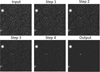 |
Fig. 1 Example of a diffusion model operation over five diffusion steps. The input is preprocessed, and between step four and output the model performs prediction and postprocessing, excluding renormalization. |
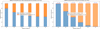 |
Fig. 2 Comparison of forward diffusion schedules in BGRem (left, this work) and the original DDPM scheme (right; Ho et al. 2020). BGRem demonstrates supervised additive corruption of the image with scaled background noise σtx, following the noise scheduling of σt described in Eq. (3). The bars represent relative contribution of photon counts from the source fraction (hatched blue) and the noise fraction (yellow) for a given time step, as obtained from a random image. |
Training and inference steps in BGRem.
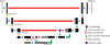 |
Fig. 3 Schematic of the backbone architecture used in BGRem, adapted from the original attention U-Net (Oktay et al. 2018). |
BGRem training hyperparameters and values.
4 Results
To quantify the performance of BGRem, we compared it with the widely used background subtraction method in SExtractor (Bertin & Arnouts 1996). The SExtractor software was developed to produce catalogs of astronomical sources using large-scale sky surveys, with background estimation and subtraction as the first steps in the pipeline. Several alternatives to SExtractor, such as ProFound (Robotham et al. 2018) and NoiseChisel (Akhlaghi & Ichikawa 2015) have been developed in recent years; however, extensive analysis (Haigh et al. 2021) shows that the performance of SExtractor is comparable to these recent alternatives, so we focus on SExtractor for analysis and comparison with BGRem. The SExtractor software models the background by estimating the local background using grids of a certain size (e.g., 64 × 64) and computing a mode (defined as mode ≈2.5× median −1.5× mean)6, of the pixel values, similar to the approach used in the Dominion Astrophysical Observatory Photometry (DAOPHOT) program (Stetson 1987). It then estimates the background via bilinear interpolation over the grid of modes in the image and subtracted it from the image.
Fig. 4 shows an example of BGRem applied to optical images with a relatively smooth background. The figure shows that the background is almost completely removed, while the sources remain intact. Beyond visual inspection, we next discuss our strategy for quantifying the performance of BGRem across the complete test set.
The distribution of pixel values in the test images, with and without background removal, by BGRem and SExtractor highlights the effectiveness of BGRem over SExtractor, as shown in Fig. 5. An image with stars and no background would have zero values in most pixels, with a tail of positive values, since stars occupy only a small portion of the image. The left panel of Fig. 5 shows that, for a test set, the histogram of pixel values obtained with BGRem closely matches this ground truth, while the histogram obtained with SExtractor is more spread out. Fig. 5, shows a zoom in on low pixel values, where background removal is most effective when comparing BGRem to SExtractor.
As mentioned above, as part of our postprocessing step, we set all pixels with values below zero to zero. This clipping induces a photometric bias for downstream tasks (such as source flux estimation), since it shifts the mean background from 0 to >0, making flux estimation, especially for fainter sources, problematic at this stage. Fig. 6 highlights the photon-count underestimation in BGRem images compared to the original images. To produce Fig. 6, we first applied BGRem to denoise the images and the applied SExtractor to localize the sources. Based on the source locations predicted by SExtractor, we cut a small region (37 × 37) centered on the predicted position from the BGRem image, given an initial patch size of 256 × 256. To determine this size, we considered two factors: first, to include larger sources (brighter and larger), the cutoff must be sufficiently large; second, it must be small enough to exclude contributions from nearby sources. We then calculated the sum of the counts within this patch as Fpred, as a proxy to measure the flux. We defined Ftrue analogously, considering the source-only cutout of the same shape. This highlights that at the current stage, BGRem cannot be used as a standalone tool to produce photometry-ready images. We used BGRem for catalog-building tasks in two steps. First, we used the BGRem output solely to generate a high-precision detection mask (building upon our previous work in Stoppa et al. 2022). We then applied this mask to the original, unclipped, background-subtracted data for final flux integration. This ensured that the statistical symmetry of the noise is preserved, providing better photometry and benefiting from a larger number of source detections (see source localization performance plots). We also note that we previously developed a more dedicated DNN-based pipeline for calculating the flux of individual sources (Stoppa et al. 2023b); however, this simple aperture photometry approach provides a sufficiently accurate proxy for our background noise removal analysis, as the full DNN-based approach is not the focus of this work.
Using BGRem as a preprocessing step can improve the performance of other applications. The source localization of SExtractor can detect more sources when BGRem is used as a preprocessing step. This is shown on a cutout from the test data. Figure 7 shows the maximum number of sources (true positives) that can be found without false positives and clearly shows that, using BGRem, eight additional sources are found in this particular example. It is also informative to examine how the model performs for different values of the SExtractor threshold (thresh) parameter, which controls the minimum significance level for source detection. When this threshold value is low, we expect to detect fainter sources (more true positives), but the number of false positives will also increase, and vice versa. Fig. 8 shows that the use of BGRem as a preprocessing step produces more true positives relative to false positives across different threshold values.
The BGRem framework also performs well on images with more complex backgrounds and smaller sizes. Fig. 9 shows an example of its generalizability to a different domain. This image was taken with MegaCam on the Canada-France–Hawaii Telescope7 (CFHT) in the g band (Heymans et al. 2012) and features part of the M31 galaxy in the background, making background removal challenging. While BGRem isolates point sources with high precision, it simultaneously demonstrates a clear limitation: the model interpreted the low-surface-brightness (LSB) structures of M31 as part of the background component and almost completely suppressed them. This aggressive removal of extended structure highlights a domain gap; because we trained our model on MeerLICHT data dominated by point sources, the attention U-Net learned to categorize any faint extended emissions as “noise”. Consequently, while the model shows strong generalizability in removing instrumental and sky backgrounds, it is currently unsuitable for preserving extended galaxies or diffuse nebular structures. This underscores that BGRem, in its current iteration, is primarily intended to improve point-source detection tasks. Since our model is trained for MeerLICHT data and no fine-tuning is applied to adapt it to this new data domain, its effectiveness in preserving point sources highlights that the model has learned generalizable features. The possibility of significant improvement through fine-tuning or training a separate BGRem model from scratch for this particular dataset is beyond the scope of this paper. Future iterations that involve multiscale loss functions or training sets with injected extended sources would likely be necessary to ensure the morphological preservation of LSB science.
To quantify the generalizability of BGRem to a dataset different from that on which it was trained, we used data from the Legacy Survey (Dey et al. 2019) obtained with the Blanco Telescope DECam instrument as part of zero-shot inference testing. We used a Flexible Image Transport System (FITS) image retrieved from the Legacy Surveys DR9 Sky Viewer tool8 to test our ML algorithm. The image, partially shown in Fig. 10, is derived from the Dark Energy Camera Legacy Survey (DECaLS) portion of the DESI Legacy Imaging Surveys from Dey et al. (2019), with and without BGRem applied. Similarly to Fig. 8, Fig. 11 plots true positives versus false positives. Even on a large cutout of real data from the Legacy Survey, we can quantify the zero-shot inference capability of BGRem and show that, across different SExtractor threshold values, BGRem performs better than the SExtractor background removal tool. We also note that for both Figs. 8 and 11, we tested the results without clipping pixel values to zero when BGRem predicts negative values. The performance of SourceExtractor to detect sources worsens in both cases.
Finally, we highlight the possibility of training BGRem to denoise astronomical images at a different wavelength with noise components distinct from those in optical images, as described above. We focus on simulated γ-ray sky images for the Fermi-LAT telescope.
Fig. 12 shows an example of BGRem performance from the test set. Fig. 12 shows two randomly selected test patches of the sky : the top panel corresponds to a region away from the Galactic plane, while the bottom panel corresponds to a region close to it. This shows that the source detection rate obtained with SExtractor on the ground-truth (source-only) image closely resembles the denoised image obtained with BGRem. We also show in Fig. 13 that the mean pixel values of the denoised images produced by BGRem follow a diagonal relation when plotted against those of the source-only images, highlighting the effectiveness of BGRem in reducing the contribution from IEM noise. A low (high) mean pixel value in the source-only image indicates that the corresponding test patch is dominated by faint (bright) sources. This demonstrates the reliability of reconstructing source pixel counts with BGRem for γ-ray images.
As with optical images, this retrained model improves the ability of SExtractor to detect sources. Fig. 14 shows this improvement. This model generates some artifacts that cause SExtractor to find false positives at very high thresholds. However, with simulated data and using SExtractor as a detection module, more than twice the number of correct sources can be identified by using BGRem as a preprocessing step, compared to the default SExtractor background removal method. We also note that, although SExtractor is not designed to remove the IEM in the γ-ray wavelength or to detect γ-ray sources, the significantly improved performance with BGRem motivates its use as a preprocessing step in current and future source detection pipelines across different wavelengths.
However, we also highlight a current limitation of BGRem in removing background noise when we include observational (Poisson) noise in the γ-ray data. Fig. 15 shows BGRem applied to the same patches as in Fig. 12s, but with added Poisson and IEM noise. This shows that, except for the brightest sources in those patches, BGRem fails to reconstruct the denoised images. To further examine the global trend, we reproduce Fig. 16, similar to Fig. 13, but include the effect of Poisson noise for the same test set used previously, and highlight how the mean pixel values of BGRem images vary relative to the original source-only images. The results show that the overall performance of BGRem degrades irrespective of the brightness of the image. A general trend that can be inferred from this is that BGRem underpredicts the counts for brighter images while over-predicting the counts for fainter images. For fainter images, BGRem struggles to distinguish between a faint real source and an upward Poisson fluctuation of the background. Thus, BGRem may interpret the noise spikes as signal and fail to subtract sufficient noise, leaving behind more counts. For brighter patches, BGRem predicts noise more aggressively, leading to the subtraction of more photon counts than optimal.
This highlights that while BGRem shows excellent promise for background removal as a proof-of-concept, the observed over- and underprediction of photon counts in the Poisson regime requires further investigation. Future work will focus on systematic hyperparameter optimization, including a more robust treatment of the image normalization factors, which are critical for the nonlinear scaling of gamma-ray counts, to ensure that the model is optimized for the stochastic nature of Poisson noise in addition to the structural complexities of the IEM.
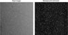 |
Fig. 4 MeerLICHT image (left) and BGRem background-removed image (right). |
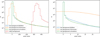 |
Fig. 5 Left: histogram of pixel values for the original simulated image (red), the ground-truth background-free image (green), SExtractor prediction (orange), and BGRem prediction (blue). Right: zoom-in of the left panel (pixel value 0–25) highlighting the close agreement between BGRem and the simulation. |
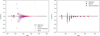 |
Fig. 6 Left: ratio of predicted flux (Fpred) to true flux (Ftrue) for BGRem (blue), SExtractor (red), and the input image (yellow), compared to the ideal line (black) as a function of the signal-to-noise ratio (S/N). Points represent individual sources: small points indicate stars, medium points galaxies, and large points elongated galaxies. Right: same as the left panel, but binned in S/N, with error bars representing statistical error. |
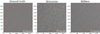 |
Fig. 7 Sources detected by SExtractor in the ground-truth image (left), the SExtractor background-subtracted image (middle), and the BGRem background-subtracted image (right). The red circles indicate the predicted shape and size of the detected sources. |
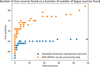 |
Fig. 8 True positives (correctly detected sources) as a function of false positives (spurious detections). Dots represent runs of source localization with varying SExtractor significance thresholds on a random cutout in the test data. |
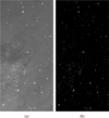 |
Fig. 9 Example of zero-shot inference withBGRem. The best model trained and tested with MeerLICHT data is directly applied to a CFHT telescope image (a) to remove the background noise and produce the denoised image (b). Image credit: CFHT / MegaCam (2022), operated by NRC Canada, CNRS France, and the University of Hawaii. Observations from Maunakea with care and respect. |
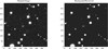 |
Fig. 10 Left: cutout from the Legacy Survey used for the source localization results shown in Fig. 11. Right: result of applying BGRem to remove background from the left image. |
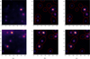 |
Fig. 12 Examples of BGRem for simulated gamma-ray sky patches for two sky regions. Top: low-IEM region away from the Galactic plane. Bottom: region with a stronger IEM component. (a) With background. (b) Source only. (c) With BGRem. The effectiveness of BGRem is highlighted by the equivalent performance of SExtractor on (b) and (c). |
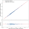 |
Fig. 13 Mean pixel values of BGRem-denoised image patches versus source-only patches (blue dots), which lie close to the diagonal line (red). Bottom: residual plot showing that BGRem reconstruction works better for brighter patches (more and/or brighter sources). |
5 Conclusions
In this paper, we introduce BGRem, a background noise remover for astronomical images. This diffusion-based model with an attention U-Net as a backbone effectively removes background noise from astronomical images with negligible artifacts. We first trained and tested BGRem on optical images from the MeerLICHT telescope and then applied domain transfer to demonstrate the effectiveness of BGRem on optical images taken by CFHT’s MegaCam and the DESI Legacy Survey on the DECam instrument. We also show that retraining the model on a different dataset, particularly for γ-ray simulated data for the Fermi-LAT telescope, provides a reliable background removal tool for astronomical images across various wavelengths. The computation does not depend on the image content, such as the number of stars or galaxies in the image. To our knowledge, this is the first time that a diffusion-based denoising model has been shown to effectively remove background from optical and γ-ray images and to improve source detection with SExtractor. Our results demonstrate that this approach serves as an effective preprocessing step for existing methods in pipelines for constructing astronomical catalogs. We also highlight the potential application of BGRem at a different wavelength, in γ-rays, where the background contamination differs from that of optical images.
However, BGRem has limitations that define its current scientific scope. As the model is trained primarily on simulations of point-like sources, it exhibits a morphological bias: the attention U-Net backbone tends to interpret diffuse, extended galaxies as part of the background component. Consequently, BGRem may attenuate signals from extended sources, making it unsuitable at present for tasks requiring surface photometry or for morphological analysis of such objects. The BGRem framework also tends to underestimate the flux of faint objects, as the model may misidentify low-level signals as a stochastic background and remove them. Thus, the direct output of BGRem should not be used for standalone high-precision photometry. Although BGRem is suitable for removing IEM noise for γ-ray data, it currently fails to model or remove Poisson noise.
Future improvements could involve fine-tuning model hyperparameters, exploring alternative noise schedules or embedding strategies, and optimizing architectural components such as attention modules. Additionally, improving the quality and diversity of the training data – through more realistic background simulations or domain-specific augmentation – could further improve BGRem’s generalization capability. We will explore these topics in future work. We also aim to apply the same technique to different training datasets to develop a model that includes astronomical images from different wavelengths, including radio, X-ray, and infrared images. Although BGRem performs robustly across different noise levels, there remains room for further improvement.
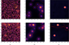 |
Fig. 15 Examples of BGRem applied to simulated gamma-ray sky patches from Fig. 12, but now including Poisson noise. (a) With background. (b) Source only. (c) With BGRem. BGRem does not fully remove Poisson noise and IEM in both high- and low-Galactic-latitude regions, highlighting a current limitation of BGRem for γ-ray data. |
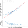 |
Fig. 16 Same as Fig. 13, but highlighting the effect of additional Poisson noise. Overall, BGRem underpredicts the counts for brighter patches and overpredicts for fainter patches. |
References
- Abadi, M., Agarwal, A., Barham, P., et al. 2015, TensorFlow: Large-scale machine learning on heterogeneous systems [Google Scholar]
- Abdollahi, S., Acero, F., Ackermann, M., et al., 2020, ApJS, 247, 33 [Google Scholar]
- Acciarri, R., Adams, C., Andreopoulos, C., et al. 2021, Front. Artif. Intell., 4, 649917 [Google Scholar]
- Acero, F., Ackermann, M., Ajello, M., et al. 2016, ApJS, 223, 26 [Google Scholar]
- Akhlaghi, M., & Ichikawa, T. 2015, ApJS, 220, 1 [Google Scholar]
- Atwood, W. B., Abdo, A. A., Ackermann, M., et al. 2009, ApJ, 697, 1071 [CrossRef] [Google Scholar]
- Bellm, E. C., Kulkarni, S. R., Graham, M. J., et al. 2018, PASP, 131, 018002 [Google Scholar]
- Bertin, E., & Arnouts, S. 1996, A&AS, 117, 393 [Google Scholar]
- Caron, S., Eckner, C., Hendriks, L., et al. 2023, J. Cosmology Astropart. Phys., 2023, 013 [Google Scholar]
- Chollet, F., et al. 2015, Keras, https://keras.io [Google Scholar]
- Croitoru, F.-A., Hondru, V., Ionescu, R. T., & Shah, M. 2023, IEEE Trans. Pattern Anal. Mach. Intell., 45, 10850 [Google Scholar]
- Dey, A., Schlegel, D. J., Lang, D., et al. 2019, AJ, 157, 168 [Google Scholar]
- Ehlert, S., Chen, C.-T., Swartz, D., et al. 2022, MNRAS, 515, 5185 [Google Scholar]
- Gheller, C., & Vazza, F. 2021, MNRAS, 509, 990 [NASA ADS] [CrossRef] [Google Scholar]
- Groot, P. J., Bloemen, S., Vreeswijk, P., et al. 2024, PASP, 136, 115003 [NASA ADS] [CrossRef] [Google Scholar]
- Haigh, C., Chamba, N., Venhola, A., et al. 2021, A&A, 645, A107 [NASA ADS] [CrossRef] [EDP Sciences] [Google Scholar]
- Heymans, C., Van Waerbeke, L., Miller, L., et al. 2012, MNRAS, 427, 146 [Google Scholar]
- Ho, J., Jain, A., & Abbeel, P. 2020, NeurIPS, 33, 6840 [Google Scholar]
- Huber, P. 1964, Ann. Math. Stat., 35, 73 [CrossRef] [Google Scholar]
- Ivezić, Ž., Kahn, S. M., Tyson, J. A., et al. 2019, ApJ, 873, 111 [Google Scholar]
- Jia, P., Lv, J., Ning, R., et al. 2023, MNRAS, 527, 6581 [Google Scholar]
- Kingma, D. P., & Ba, J. 2014, arXiv preprint [arXiv:1412.6980] [Google Scholar]
- Loshchilov, I., & Hutter, F. 2017, in ICLR [Google Scholar]
- Maas, A. L., Hannun, A. Y., & Ng, A. Y. 2013, ICML, 30 [Google Scholar]
- Oktay, O., Schlemper, J., Folgoc, L. L., et al. 2018, arXiv preprint [arXiv:1804.03999] [Google Scholar]
- Panes, B., Eckner, C., Hendriks, L., et al. 2021, A&A, 656, A62 [NASA ADS] [CrossRef] [EDP Sciences] [Google Scholar]
- Robotham, A. S. G. 2018, MNRAS, 476, 3137 [NASA ADS] [CrossRef] [Google Scholar]
- Ronneberger, O., Fischer, P., & Brox, T. 2015, in MICCAI-2015 (Springer International Publishing), 234 [Google Scholar]
- Roscani, V., Tozza, S., Castellano, M., et al. 2020, A&A, 643, A43 [NASA ADS] [CrossRef] [EDP Sciences] [Google Scholar]
- Rowe, B. T., Jarvis, M., Mandelbaum, R., et al. 2015, Astron. Comput., 10, 121 [NASA ADS] [CrossRef] [Google Scholar]
- Sohl-Dickstein, J., Weiss, E., Maheswaranathan, N., & Ganguli, S. 2015, in ICML, PMLR, 2256 [Google Scholar]
- Song, Y., Sohl-Dickstein, J., Kingma, D. P., et al. 2020, ICML [Google Scholar]
- Stetson, P. B. 1987, PASP, 99, 191 [Google Scholar]
- Stoppa, F., Vreeswijk, P., Bloemen, S., et al. 2022, A&A, 662, A109 [NASA ADS] [CrossRef] [EDP Sciences] [Google Scholar]
- Stoppa, F., Bhattacharyya, S., de Austri, R. R., et al. 2023a, A&A, 680, A109 [NASA ADS] [CrossRef] [EDP Sciences] [Google Scholar]
- Stoppa, F., de Austri, R. R., Vreeswijk, P., et al. 2023b, A&A, 680, A108 [NASA ADS] [CrossRef] [EDP Sciences] [Google Scholar]
- Tian, C., Fei, L., Zheng, W., et al. 2020, Neural Netw., 131, 251 [Google Scholar]
- Tung, Y.-C., Li, J., et al. 2024, Nucl. Instrum. Methods Phys. Res. A, 1059, 169010 [Google Scholar]
- van den Oetelaar, C., Bhattacharyya, S., Panes, B., et al. 2021, PoS, ICRC, 663 [Google Scholar]
- Vaswani, A., Shazeer, N., Parmar, N., et al. 2017, NeurIPS, 30 [Google Scholar]
- Vojtekova, A., Lieu, M., Valtchanov, I., et al. 2020, MNRAS, 503, 3204 [Google Scholar]
- Wolf, T. N., Jones, B. A., & Bowler, B. P. 2024, AJ, 167, 92 [Google Scholar]
- Zackay, B., & Ofek, E. O. 2017a, ApJ, 836, 187 [Google Scholar]
- Zackay, B., & Ofek, E. O. 2017b, ApJ, 836, 188 [Google Scholar]
Appendix A Acknowledgements
We would like to thank the anonymous referee for constructive comments and queries which have made the draft overall better. The authors are grateful to P.M. Vreeswijk for helpful comments to improve the draft. The work of S.B was supported by the Slovenian Research Agency under grants P1-0031, N1-0344, and J1-60014. PJG is partly supported by NRF SARChI grant 111692. The work of R. RdA was supported by PID2020-113644GB-I00 from the Spanish Ministerio de Ciencia e Innovación and by the PROMETEO/2022/69 from the Spanish GVA. The Legacy Surveys consist of three individual and complementary projects: the Dark Energy Camera Legacy Survey (DECaLS; Proposal ID #2014B-0404; PIs: David Schlegel and Arjun Dey), the Beijing-Arizona Sky Survey (BASS; NOAO Prop. ID #2015A-0801; PIs: Zhou Xu and Xiaohui Fan), and the Mayall z-band Legacy Survey (MzLS; Prop. ID #2016A-0453; PI: Arjun Dey). DECaLS, BASS and MzLS together include data obtained, respectively, at the Blanco telescope, Cerro Tololo Inter-American Observatory, NSF’s NOIRLab; the Bok telescope, Steward Observatory, University of Arizona; and the Mayall telescope, Kitt Peak National Observatory, NOIRLab. Pipeline processing and analyses of the data were supported by NOIRLab and the Lawrence Berkeley National Laboratory (LBNL). The Legacy Surveys project is honored to be permitted to conduct astronomical research on Iolkam Du’ag (Kitt Peak), a mountain with particular significance to the Tohono O’odham Nation. NOIRLab is operated by the Association of Universities for Research in Astronomy (AURA) under a cooperative agreement with the National Science Foundation. LBNL is managed by the Regents of the University of California under contract to the U.S. Department of Energy. This project used data obtained with the Dark Energy Camera (DECam), which was constructed by the Dark Energy Survey (DES) collaboration. Funding for the DES Projects has been provided by the U.S. Department of Energy, the U.S. National Science Foundation, the Ministry of Science and Education of Spain, the Science and Technology Facilities Council of the United Kingdom, the Higher Education Funding Council for England, the National Center for Supercomputing Applications at the University of Illinois at Urbana-Champaign, the Kavli Institute of Cosmological Physics at the University of Chicago, Center for Cosmology and Astro-Particle Physics at the Ohio State University, the Mitchell Institute for Fundamental Physics and Astronomy at Texas A&M University, Financiadora de Estudos e Projetos, Fundacao Carlos Chagas Filho de Amparo, Financiadora de Estudos e Projetos, Fundacao Carlos Chagas Filho de Amparo a Pesquisa do Estado do Rio de Janeiro, Conselho Nacional de Desenvolvimento Cientifico e Tecnologico and the Ministerio da Ciencia, Tecnologia e Inovacao, the Deutsche Forschungsgemeinschaft and the Collaborating Institutions in the Dark Energy Survey. The Collaborating Institutions are Argonne National Laboratory, the University of California at Santa Cruz, the University of Cambridge, Centro de Investigaciones Energeticas, Medioambientales y Tecnologicas-Madrid, the University of Chicago, University College London, the DES-Brazil Consortium, the University of Edinburgh, the Eidgenossische Technische Hochschule (ETH) Zurich, Fermi National Accelerator Laboratory, the University of Illinois at Urbana-Champaign, the Institut de Ciencies de l’Espai (IEEC/CSIC), the Institut de Fisica d’Altes Energies, Lawrence Berkeley National Laboratory, the Ludwig Maximilians Universitat Munchen and the associated Excellence Cluster Universe, the University of Michigan, NSF’s NOIRLab, the University of Nottingham, the Ohio State University, the University of Pennsylvania, the University of Portsmouth, SLAC National Accelerator Laboratory, Stanford University, the University of Sussex, and Texas A&M University. BASS is a key project of the Telescope Access Program (TAP), which has been funded by the National Astronomical Observatories of China, the Chinese Academy of Sciences (the Strategic Priority Research Program “The Emergence of Cosmological Structures” Grant # XDB09000000), and the Special Fund for Astronomy from the Ministry of Finance. The BASS is also supported by the External Cooperation Program of Chinese Academy of Sciences (Grant # 114A11KYSB20160057), and Chinese National Natural Science Foundation (Grant # 12120101003, # 11433005). The Legacy Survey team makes use of data products from the Near-Earth Object Wide-field Infrared Survey Explorer (NEOWISE), which is a project of the Jet Propulsion Laboratory/California Institute of Technology. NEOWISE is funded by the National Aeronautics and Space Administration. The Legacy Surveys imaging of the DESI footprint is supported by the Director, Office of Science, Office of High Energy Physics of the U.S. Department of Energy under Contract No. DE-AC02-05CH1123, by the National Energy Research Scientific Computing Center, a DOE Office of Science User Facility under the same contract; and by the U.S. National Science Foundation, Division of Astronomical Sciences under Contract No. AST-0950945 to NOAO. Based on observations obtained with MegaPrime/MegaCam, a joint project of CFHT and CEA/DAPNIA, at the Canada-France-Hawaii Telescope (CFHT), which is operated by the National Research Council (NRC) of Canada, the Institut National des Sciences de 1’Univers of the Centre National de la Recherche Scientifique (CNRS) of France, and the University of Hawaii. The observations at the CFHT were performed with care and respect from the summit of Maunakea, which is a significant cultural and historic site. The MeerLICHT telescope is designed, installed and operated by a consortium including Radboud University, the University of Cape Town, the University of Oxford, the University of Manchester, the University of Amsterdam, and the South African Astronomical Observatory, a part of the South African National Science Foundation.
Appendix B BGRem hyper-parameters: Normalization factor and diffusion steps
To get the best results with BGRem, here we discuss the choices of the two hyperparameters that might affect the performance. First, the normalization factor, which determines how well the background gets removed. Since the noise in the training data is likely different from the one encountered in most real images, we have to make them match as well as possible. This is done by tuning the normalization factor in such a way that the noise has a standard deviation of around 1. The mean of the noise isn’t important since this is removed in one of the preprocessing steps. Setting the normalization factor too low will result in the model recognizing faint stars as background and removing them, while setting it too high will result in the model seeing the background as sources and not removing it. This is shown in Fig. B.1.
BGRem has a built-in tool that can estimate the normalization factor by calculating the standard deviation σ of the pixel values. Stars heavily influence this, so it ignores the 10% brightest pixels. It also ignores all pixels with a value of 0 if there are any, so it doesn’t take into account empty parts of images. The normalization factor is then simply ![Mathematical equation: $\[\frac{1}{\sigma}\]$](/articles/aa/full_html/2026/06/aa57715-25/aa57715-25-eq16.png) . This works best for an image with a uniform background and might need tuning for images with large gradients in the background.
. This works best for an image with a uniform background and might need tuning for images with large gradients in the background.
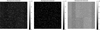 |
Fig. B.1 Effect of a good normalization factor (left), a too low normalization factor (middle) and a too high normalization factor (right) on the output of the model. |
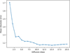 |
Fig. B.2 Mean absolute error of BGRem on the validation data as a function of the number of diffusion steps. |
The second parameter of BGRem is the number of diffusion steps. This determines how many steps the diffusion model removes the background. The accuracy increases with the increasing number of steps, but the computation time also increases linearly. Figure B.2 shows the mean absolute error of the model as a function of the number of diffusion steps. This was tested on the validation data.
Here we see that even with only one diffusion step, the model is very accurate. However, with more diffusion steps, the model is less likely to introduce image artifacts, making the performance even better. The optimal performance is at 15 diffusion steps, while 3, 6 and 11 are local optima, making these four choices preferable over other options.
Appendix C Effect of training with MSE loss
While in our work to train BGRem we have used MAE loss, in the original DDPM work, L2/MSE loss was introduced (Ho et al. 2020). First, we checked from reconstructed image quality inspection that MSE loss fails to properly remove the background. This can be visually seen for reference images in optical dataset trained with MAE and MSE loss (top and bottom row of Fig. C.1 respectively). The same can be seen for the γ-ray images as shown in Fig. C.2 and compared to the results presented before in Fig. 12. Also, we quantify by plotting the mean pixel values of the de-noised images with BGRem against the mean pixel values of the source-only images in Fig. C.3, which can be compared to Fig. 13 presented before obtained with MAE loss. While for the brighter patches, even with MSE loss BGRem performance is similar to that of obtained with MAE loss, for the fainter patches the performance is significantly worse, which can be seen from the residuals.
In the original DDPM work, during the forward process the image is completely destroyed and usually we have a Gaussian noise with zero mean and unit variance ϵ ~ (𝒩(0, 𝕀)). Minimizing the MSE loss is a natural consequence of maximum likelihood under Gaussian Noise. For astronomical images with backgrounds (noise) we may have bright structures, localized excess, occasional extreme flares and these can be grouped into outliers; MAE penalizes error linearly and is less sensitive to outliers. While MAE performs better according to our tests, for our future work, we intend to test BGRem with Huber loss (Huber 1964) where it can seamlessly move from MSE to MAE depending on the small to large error values.
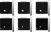 |
Fig. C.1 Example of training BGRem with MAE loss for a random MeerLICHT image (top row) compared with MSE loss (bottom row). Visually inspecting the final column where we obtain the ‘cleaned’ image with BGRem highlights that training with MSE loss fails to remove background properly. |
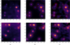 |
Fig. C.2 Examples of BGRem for the same simulated gamma-ray sky patches as in Fig. 12, but now obtained with MSE loss. Panel (a): With background. Panel (b): Source only. Panel (c): With BGRem. It fails to properly remove the background noise and produces artifacts, highlighting MSE loss being less effective than MAE. |
All Tables
All Figures
|
Fig. 1 Example of a diffusion model operation over five diffusion steps. The input is preprocessed, and between step four and output the model performs prediction and postprocessing, excluding renormalization. |
| In the text | |
|
Fig. 2 Comparison of forward diffusion schedules in BGRem (left, this work) and the original DDPM scheme (right; Ho et al. 2020). BGRem demonstrates supervised additive corruption of the image with scaled background noise σtx, following the noise scheduling of σt described in Eq. (3). The bars represent relative contribution of photon counts from the source fraction (hatched blue) and the noise fraction (yellow) for a given time step, as obtained from a random image. |
| In the text | |
|
Fig. 3 Schematic of the backbone architecture used in BGRem, adapted from the original attention U-Net (Oktay et al. 2018). |
| In the text | |
|
Fig. 4 MeerLICHT image (left) and BGRem background-removed image (right). |
| In the text | |
|
Fig. 5 Left: histogram of pixel values for the original simulated image (red), the ground-truth background-free image (green), SExtractor prediction (orange), and BGRem prediction (blue). Right: zoom-in of the left panel (pixel value 0–25) highlighting the close agreement between BGRem and the simulation. |
| In the text | |
|
Fig. 6 Left: ratio of predicted flux (Fpred) to true flux (Ftrue) for BGRem (blue), SExtractor (red), and the input image (yellow), compared to the ideal line (black) as a function of the signal-to-noise ratio (S/N). Points represent individual sources: small points indicate stars, medium points galaxies, and large points elongated galaxies. Right: same as the left panel, but binned in S/N, with error bars representing statistical error. |
| In the text | |
|
Fig. 7 Sources detected by SExtractor in the ground-truth image (left), the SExtractor background-subtracted image (middle), and the BGRem background-subtracted image (right). The red circles indicate the predicted shape and size of the detected sources. |
| In the text | |
|
Fig. 8 True positives (correctly detected sources) as a function of false positives (spurious detections). Dots represent runs of source localization with varying SExtractor significance thresholds on a random cutout in the test data. |
| In the text | |
|
Fig. 9 Example of zero-shot inference withBGRem. The best model trained and tested with MeerLICHT data is directly applied to a CFHT telescope image (a) to remove the background noise and produce the denoised image (b). Image credit: CFHT / MegaCam (2022), operated by NRC Canada, CNRS France, and the University of Hawaii. Observations from Maunakea with care and respect. |
| In the text | |
|
Fig. 10 Left: cutout from the Legacy Survey used for the source localization results shown in Fig. 11. Right: result of applying BGRem to remove background from the left image. |
| In the text | |
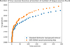 |
Fig. 11 Same as Fig. 8, but applied to real data from the Legacy Survey. |
| In the text | |
|
Fig. 12 Examples of BGRem for simulated gamma-ray sky patches for two sky regions. Top: low-IEM region away from the Galactic plane. Bottom: region with a stronger IEM component. (a) With background. (b) Source only. (c) With BGRem. The effectiveness of BGRem is highlighted by the equivalent performance of SExtractor on (b) and (c). |
| In the text | |
|
Fig. 13 Mean pixel values of BGRem-denoised image patches versus source-only patches (blue dots), which lie close to the diagonal line (red). Bottom: residual plot showing that BGRem reconstruction works better for brighter patches (more and/or brighter sources). |
| In the text | |
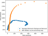 |
Fig. 14 Same as Figs. 8 and 11, but for results obtained with simulated γ-ray sky images. |
| In the text | |
|
Fig. 15 Examples of BGRem applied to simulated gamma-ray sky patches from Fig. 12, but now including Poisson noise. (a) With background. (b) Source only. (c) With BGRem. BGRem does not fully remove Poisson noise and IEM in both high- and low-Galactic-latitude regions, highlighting a current limitation of BGRem for γ-ray data. |
| In the text | |
|
Fig. 16 Same as Fig. 13, but highlighting the effect of additional Poisson noise. Overall, BGRem underpredicts the counts for brighter patches and overpredicts for fainter patches. |
| In the text | |
|
Fig. B.1 Effect of a good normalization factor (left), a too low normalization factor (middle) and a too high normalization factor (right) on the output of the model. |
| In the text | |
|
Fig. B.2 Mean absolute error of BGRem on the validation data as a function of the number of diffusion steps. |
| In the text | |
|
Fig. C.1 Example of training BGRem with MAE loss for a random MeerLICHT image (top row) compared with MSE loss (bottom row). Visually inspecting the final column where we obtain the ‘cleaned’ image with BGRem highlights that training with MSE loss fails to remove background properly. |
| In the text | |
|
Fig. C.2 Examples of BGRem for the same simulated gamma-ray sky patches as in Fig. 12, but now obtained with MSE loss. Panel (a): With background. Panel (b): Source only. Panel (c): With BGRem. It fails to properly remove the background noise and produces artifacts, highlighting MSE loss being less effective than MAE. |
| In the text | |
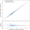 |
Fig. C.3 Same as Fig. 13 but now with MSE loss. |
| In the text | |
Current usage metrics show cumulative count of Article Views (full-text article views including HTML views, PDF and ePub downloads, according to the available data) and Abstracts Views on Vision4Press platform.
Data correspond to usage on the plateform after 2015. The current usage metrics is available 48-96 hours after online publication and is updated daily on week days.
Initial download of the metrics may take a while.