| Issue |
A&A
Volume 709, May 2026
|
|
|---|---|---|
| Article Number | A133 | |
| Number of page(s) | 13 | |
| Section | Numerical methods and codes | |
| DOI | https://doi.org/10.1051/0004-6361/202558042 | |
| Published online | 08 May 2026 | |
Multi-scale learning with point spread function and spectral energy distribution constraints for faint source detection in lobster-eye X-ray telescopes
1
Key Laboratory of Space Astronomy and Technology, National Astronomical Observatories, Chinese Academy of Sciences,
Beijing
100101,
China
2
University of Chinese Academy of Sciences,
Beijing
100049,
China
★ Corresponding authors: This email address is being protected from spambots. You need JavaScript enabled to view it.
; This email address is being protected from spambots. You need JavaScript enabled to view it.
Received:
10
November
2025
Accepted:
9
March
2026
Abstract
Context. Detecting faint and cross-shaped sources in long-exposure images from lobster-eye X-ray telescopes is particularly challenging due to the low signal-to-noise ratio (S/N), complex noise, and unique point spread function (PSF) of these instruments. Conventional deep learning networks struggle in such conditions as they fail to effectively incorporate astrophysical priors such as photon arrival time, energy, and PSF morphology. Furthermore, the significant flux-scale differences between faint and bright sources complicate feature extraction in the standard feature pyramid network (FPN).
Aims. The goal is to propose a PSF-guided multi-scale detection framework that integrates prior physical features and is specifically designed for the Wide-field X-ray Telescope (WXT) on board the Einstein Probe (EP).
Methods. Our approach began by constructing three-channel inputs, combining conventional grayscale images with photon energy and arrival time data. We then introduced a PSF-guided morphological convolution module (PSFConv) and a multi-kernel multi-scale FPN (MKMS-FPN) to enhance the extraction of morphological features and improve multi-scale target perception. Additionally, we integrated high-level convolutional features with prior physical statistics within a multibranch binary classifier of our detection network to boost both detection sensitivity and interpretability.
Results. Using simulated long-exposure WXT data and in-orbit EP observations, our framework achieves 90% precision with recall rates of 0.85 and 0.95 for sources with flux >2 mCrab (i.e. 3.21 × 10⁻¹¹ erg cm−2 s−1, unabsorbed, 0.5-4 keV) and flux >3 mCrab, respectively. At moderate precision levels, the framework further doubles the number of detectable sources with flux < 1 mCrab compared to conventional CNNs and the SExtractor pipeline.
Conclusions. The integration of physical priors with deep convolutional features demonstrates a robust detection performance across diverse flux regimes. The proposed framework offers a practical reference for data processing in future lobster-eye X-ray missions, promising enhanced sensitivity for detecting faint sources in challenging astrophysical observations.
Key words: methods: data analysis / techniques: image processing / X-rays: general
© The Authors 2026
 Open Access article, published by EDP Sciences, under the terms of the Creative Commons Attribution License (https://creativecommons.org/licenses/by/4.0), which permits unrestricted use, distribution, and reproduction in any medium, provided the original work is properly cited.
This article is published in open access under the Subscribe to Open model. This email address is being protected from spambots. You need JavaScript enabled to view it. to support open access publication.
1 Introduction
Lobster-eye X-ray telescopes have emerged as key facilities for time-domain X-ray astronomy because they deliver arcminutelevel imaging across thousands of square degrees using micropore optics (MPO) that focus soft X-rays at grazing incidence. The Einstein Probe (EP, Yuan et al. 2015, 2018; Yuan et al. 2022, 2025) mission achieves this 3850 square degrees with its Wide-field X-ray Telescope (WXT), enabling systematic monitoring of both bright transients and weak persistent emitters over an instantaneous field of view of ≳103 deg2. The technology builds on the original lobster-eye concept (Angel 1979) and was space-qualified by the EP pathfinder LEIA, which produced the first truly wide-field focusing X-ray images in orbit and validated the characteristic cruciform point spread function (PSF) and near-uniform effective area across the field (Ling et al. 2023; Zhang et al. 2022). However, robust point-source detection across such wide fields is nontrivial, since the square-pore MPO produces field-dependent aberrations and highly non-Gaussian, cross-shaped PSFs with extended arms (Cheng et al. 2024; Cheng et al. 2026, 2025b), together with complex noise distributions, all of which degrade the performance of simple aperture photometry and classical sliding-cell methods.
Moreover, the diverse spatial scales and temporal durations of sources, ranging from compact point-like emitters to extended diffuse structures, from short-timescale events (e.g., short gamma ray bursts) to long-duration phenomena (e.g., outbursts of X-ray binaries, tidal disruption events), further complicate source extraction and classification, particularly in deep exposures. Zuo et al. (2024) proposed a machine learning approach for classifying X-ray sources based on extracted parameters from LEIA data. While effective for catalog-level analysis, their method assumes prior source detection and does not address the challenges of direct detection under low signal-to-noise ratio (S/N) and complex PSF conditions, which are the focus of this study.
Astronomical object detection, particularly for faint sources in high-noise environments, remains one of the major challenges in observational astronomy. Traditional methods, such as thresholding and background subtraction, can be effective for detecting relatively bright sources in low-noise environments, but they often struggle in situations in which background noise overwhelms faint signals (Benezeth et al. 2010; Geological 2024). This issue is particularly pertinent in the case of X-ray astronomy, where long exposure times and low S/N make it increasingly difficult to detect faint sources. As exposure time increases, the background noise grows following a square root relationship, while the signal intensity increases linearly, making it harder to distinguish weak sources (Jeffs et al. 2008; Lucke & Kessel 2006). This problem is exacerbated by the inherent characteristics of X-ray telescopes, particularly those utilizing lobster-eye optics, where the faint sources are often spatially extended and have complex structural features (Van Inneman et al. 1999; Feng et al. 2024). Sawano et al. (2020) reduced threshold dependence by overlapping two regions of interest (ROIs). However, the method relies on 1D data, limiting its ability to handle complex scenes and PSF distortions. It also fails to enhance PSF shape feature extraction and struggles to apply an integral detection threshold across targets of different scales. Jia et al. (2023) introduced a two-stage machine learning framework for lobster-eye X-ray telescopes, which mitigates the masking effect of bright sources on faint targets through patch-based multi-scale detection. While this strategy improves target separation, it does not explicitly address how convolutional networks can be adapted to enhance sensitivity to the PSF morphology or improve feature extraction for faint, low-S/N sources.
Building on this, Nammour et al. (2022) introduced a shape-constrained loss within a deep learning framework to improve galaxy image deconvolution, explicitly preserving morphological fidelity such as galaxy shapes and flux. Yang et al. (2025) introduced a pinwheel-shaped convolution that better captures the spatial structure of small infrared targets by aligning with their radial pixel distribution. Inspired by this, we introduce a morphology-inspired convolutional structure that emulates the PSF of lobster-eye telescopes, allowing the network to better capture the spatial and structural features that are inherent to the target objects. Furthermore, we incorporate a multi-kernel convolution structure within the FPN to account for the scale differences in target sizes. The multi-kernel convolution structure (Chen et al. 2025; Xiao et al. 2025) has been shown to effectively capture multi-scale contextual information and enhance feature discrimination across varying target sizes. Building upon this property, we further introduce a channel-aware enhancement mechanism within the FPN, aiming to improve the representation of scale-varying targets.
Additionally, our hybrid classifier model, which integrates deep features derived from CNNs with prior physical knowledge, provides a robust and interpretable detection framework for X-ray astronomy. This model combines high-level CNN feature maps with key astrophysical parameters, such as source morphology and physical parameters, alongside prior image statistics. This integration allows the model to effectively handle complex X-ray data, including low-S/N and spatially extended sources, while improving source detection accuracy.
The remainder of this paper is organized as follows. Sect. 2 introduces the data used and the dataset production process. Sect. 3 describes the detection framework. The experimental results and analyses are provided in Sect. 4. We draw conclusions in Sect. 5.
2 Data
Sect. 2.1 introduces the sources and relevant information in this study. The data preprocessing procedures, including channel expansion and data enhancement are described in Sect. 2.2.
2.1 Data sources
In this study, we use simulated data from a Monte Carlobased simulator developed by the EP team, along with real observational images from EP after calibration. The simulator models photon and electron noise accounting for the capability of the telescope, including the variations in the PSF and detector response. The X-ray sources are mainly sourced from the ROSAT All-Sky Survey Bright Source Catalog (Voges et al. 1999). A simplified version of the simulator is publicly available on the EP website1 The fidelity of these simulations has been validated against early in-orbit data from the LEIA pathfinder mission (Zhang et al. 2022).
The simulated data includes four components: arrival time, photon energy, and the x and y photon coordinates on the detector plane. Exposure times range from 1500 to 2500 seconds, and the X-ray photons are distributed across a 4096×4096 pixel detector, with energies of between 0.5 keV and 4 keV. The grayscale values in the 2D images correspond to detected photons along specific directions. While these data are initially stacked into 2D images, deep learning models typically require three-channel RGB-like inputs, which may result in a loss of essential physical information when adapting the simulation data for model input.
Real observational images from the EP exhibit distinct physical features of X-ray sources, especially high-flux sources that often display extended, cross-shaped arms spanning significant portions of the image. These extended structures are particularly challenging for detection algorithms, as they may lead to fragmentation or incomplete detection. On the other hand, medium- and low-flux sources exhibit lower S/Ns and are distributed over larger areas, leading to lower pixel values. Low flux or low-count-rate sources further exacerbate PSF blurring, as the reduced S/N makes it difficult to recover sharp details, especially during deconvolution or PSF-based detection processes (Selig & Enßlin 2015; Westerkamp et al. 2024). Such conditions introduce significant challenges for accurate image reconstruction and source detection. Additionally, the low S/N in such images poses a significant challenge for detection algorithms, as it increases the likelihood of false positives and negatives (Soltan 2010). To mitigate these challenges, we employed data preprocessing techniques to enhance the S/N and optimize the dataset for subsequent deep learning analysis.
2.2 Data preprocessing
In standard computer vision tasks, CNNs expect three-channel RGB inputs, so astronomical images are often duplicated into pseudo-three-channel grayscale images. However, this replication introduces no new information and discards the physical content of event-level data, such as photon energy and arrival time. To address this, we constructed a physics-driven three-channel representation, as is shown in Fig. 2.
In the data processing phase, we generated grayscale images from the 4D simulated data containing spatial coordinates, arrival time, and photon energy. Additionally, we applied an energy-domain filtering based on the photon PI values, which restricts photons to the statistically dominant energy range and suppresses background-dominated events, thereby enhancing the S/N. Moreover, we investigated flux, measured in millicrab, as an effective parameter for constructing image datasets. Band et al. (1993) introduced the Band function for gamma-ray burst spectra and Preece et al. (2000) analyzed high-resolution detector data over 28-1800 keV. Zhang & Meszaros (2004) reported a low-energy power-law index, α, peaking near −1 with integrated slopes near −2 consistent with the theory. Based on these studies, we analyzed the flux distributions in EP data. Fig. 1 suggests that photon statistical features and power-law spectral slopes contain meaningful information that can complement traditional image-based inputs. However, variability occurs due to incomplete background subtraction, photon noise, and other observational uncertainties, with instrumental noise and limited photon statistics causing fluctuations that do not entirely obscure the theoretical trend (Salmon et al. 2014).
For each observation, we first applied an energy-domain filtering based on the photon PI distribution, retaining only photon events within the 3-sigma energy range. From the filtered event list, three complementary channels are constructed. The first channel is the grayscale photon count map that represents the spatial distribution of detected photons. The second channel is a PI-weighted map, where each pixel is weighted by the mean PI value of its photons, emphasizing spectrally harder and brighter regions. The third channel encodes temporal-spectral behavior through a local power-law-like slope derived from photon arrival times.
An innovation lies in the temporal segmentation of the entire exposure into overlapping time-series segments (with 25% overlap). The temporal segments are defined as overlapping windows of the total exposure, and then features from all segments are fused so that the full photon statistics are preserved. This allows the network to model temporal background evolution without fragmenting the source signal or losing photons and effectively transforms a long-integration image into a shortduration image sequence, enhancing temporal coherence and mitigating the low S/N inherent in individual short exposures.
By combining spatial, spectral, and temporal information into a multichannel image sequence, we provide the CNN with a structured and physically meaningful representation of the data. This enables the network to learn features correlated with variability timescales and spectral signatures, critical for distinguishing astrophysical sources from background noise and for identifying multi-scale targets in high-energy observations.
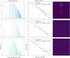 |
Fig. 1 Photon statistics and spectral properties of a typical brightness sample. The left panel shows the photon count distribution, with flux represented on a logarithmic scale. The middle panel presents the linear fit of the power-law spectral slope, which aligns with the theoretical expectations for gamma-ray burst spectra, though noise causes significant fluctuations. The right panel displays the spatial distribution of photon points on the detector plane, enhanced using a logarithmic scaling for better visibility. |
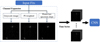 |
Fig. 2 Data processing workflow for CNN input: raw FITS images are expanded into three channels: the original grayscale image, a photon weighted map, and a power-law spectral slope map based on photon arrival times. These are segmented into overlapping time windows, creating a sequence of frames with temporal features for CNN input. |
 |
Fig. 3 Detection framework architecture. Based on a Faster R-CNN backbone, the model integrates two key components: (1) PSF-guided morphological convolution for improved feature extraction, and (2) multi-scale FPN for enhanced spatial feature representation. Together, these form an integrated end-to-end pipeline for astronomical object detection. |
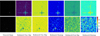 |
Fig. 4 Feature maps and heat maps across ResNet50 bottlenecks show that increasing depth (e.g., Bottleneck4 to Bottleneck6) does not improve focus on faint cross-shaped sources. Instead, deeper layers exhibit diffuse attention and amplified noise, reducing feature distinctness. |
3 Detection framework
This section introduces the faint source detection framework. To achieve this goal, we adopted a two-stage detection network based on Faster R-CNN, integrating a PSF-guided morphological convolution module (PSFConv) and a multi-kernel multi-scale feature pyramid network (MKMS-FPN). The overall framework is further illustrated in Fig. 3. In Sect. 3.1, a convolution layer with wavelet filters simulates the cross-shaped structure of the PSF, enhancing feature extraction from astronomical PSF morphology. Sect. 3.2 introduces the MKMS-FPN, which uses channel splitting and multi-scale convolutions to improve spatial feature representation and balance contributions from targets across different scales. Sect. 3.3 presents a loss function incorporating morphology-based constraints, boosting the model’s ability to capture relevant features. Finally, in Sect. 3.4, high-level convolutional features and physics-based features are combined to form joint representations, which are then fed into the binary classifier in the ROI head to discriminate true sources from the background for final detection.
3.1 Morphological convolution
We first analyzed the feature maps and heat maps and class activation mappings (CAMs) of deep networks, using ResNet50 as an example. In convolutional networks, a “bottleneck” block refers to a residual module designed to reduce computational cost while preserving information through skip connections. Here, Bottleneck4 and Bottleneck6 denote the fourth and sixth such modules within the network, corresponding to mid- and high-level feature representations. As is shown in Fig. 4, the heat maps indicate that red regions correspond to higher network attention. These visualizations reveal that increasing depth from Bottleneck4 to Bottleneck6 does not enhance the focus on target sources. Instead, the later stage shows a more diffuse activation, failing to concentrate on critical regions containing faint sources. Furthermore, while Bottleneck6 captures more abstract patterns, it also amplifies background noise and introduces greater feature degradation, complicating the discernment of true astronomical signals. These results suggest that simply deepening standard convolutional networks may weaken localization capability and reduce feature distinctness for faint source detection. Therefore, we propose a wavelet filtered morphological convolution structure tailored for cross-shaped faint sources in lobster-eye telescope observations.
To address challenges in weak signal feature extraction and morphological restoration, we propose a novel convolutional structure integrating wavelet convolution and PSFConv, inspired by the design philosophy of morphological convolutions that emphasize preserving structural priors and shape cues, so as to better capture faint features without overly smoothing edges (Yang et al. 2025; Cui et al. 2025), whose morphological effect is illustrated in Fig. 5. Furthermore, to bridge the gap between the high-level framework in Fig. 3 and the operator-level illustration in Fig. 5, we further provide a detailed backbone specification in Fig. 6, which explicitly presents the layer-wise architecture, channel dimensions, and the integration of PSFConv and the wavelet transformer within the feature extraction network.
The process begins with a wavelet transform, which decomposes the input image into low-frequency and multiple high-frequency components using wavelet bases. This decomposition enables effective signal-noise separation and multi-scale feature extraction, isolating the low-frequency contours and high-frequency details of the target. The feature map is then processed by the PSFConv module, which uses a pinwheel-shaped convolution kernel with four-fold central symmetry. This kernel is designed to capture directional spatial information, specifically adapting to the cross-shaped spatial diffusion characteristics of astronomical targets. Through parallel convolutions in four directions, PSFConv enhances the contribution of photons from each direction to the central region, thereby expanding the receptive field of the target area for more precise capture of its morphology and texture.
By combining a PSF-guided convolutional structure with a wavelet transform, our approach not only retains the shape and boundary sensitivity inherent in morphological convolutional designs, but also incorporates the physical prior of the PSF. This dual integration enables the network to enhance both frequency-domain details and spatial structural consistency, thereby achieving more accurate morphological recovery and weak signal detection across multiple scales and under complex background conditions.
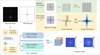 |
Fig. 5 Wavelet-enhanced PSF-guided morphological convolution. After decomposing the input into multi-scale frequency components via wavelet transform, the model applies a cross-shaped convolutional structure that conforms to the morphology of astronomical PSFs, particularly the extended arms. This design aggregates dispersed information along the PSF pattern toward the central region, thereby enhancing weak, extended features. The receptive field visualization illustrates how this morphological structure enlarges the perception range and improves sensitivity to cross-shaped sources. |
3.2 Multi-scale detection strategy
In the subsequent feature enhancement structure, we designed a MKMS-FPN to strengthen the representation of astronomical sources with variable spatial extents and morphological complexity. As is illustrated in Fig. 7, the core design principle is to decouple spatial and semantic information through an attention mechanism, and to aggregate contextual evidence across multiple receptive fields via parallel convolutional kernels of different sizes that allow the model to probe multiple spatial scales simultaneously, ensuring that neither small faint sources nor extended cross-arm structures are suppressed by a single fixed kernel size.
While Fig. 7 highlights the conceptual design and its effect on multi-scale feature extraction, the concrete implementation of MKMS-FPN within the detection backbone is shown in Fig. 8. In this architecture, feature maps from different backbone stages (C2-C4) are projected to a unified channel dimension and fused through a top-down pathway with lateral connections, forming pyramid levels P2-P5.
The pyramid features are enhanced through multi-scale aggregation and attention-based refinement, which improves their representation before being passed to the region proposal network (RPN). The RPN generates candidate source regions at different spatial scales, and these proposals are then aligned with the pyramid features using ROI pooling, producing fixed-size representations for subsequent classification and localization tasks.
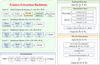 |
Fig. 6 Detailed architecture of the feature extraction backbone. The network consists of four hierarchical stages. An initial feature extraction block maps the input from 3 to 64 channels and integrates a wavelet transformer and a PSF-guided pinwheel convolution (PSFConv) to preserve multi-scale frequency information and PSF-aligned morphology. Each stage is built from residual bottleneck blocks with CBAM attention for adaptive feature refinement. The PSFConv module applies four directional convolutions (two horizontal and two vertical) followed by fusion to model the cross-shaped PSF structure of Lobster-Eye optics. The wavelet transformer decomposes features into four subbands, processes them via grouped convolution, and reconstructs the spatial representation via inverse wavelet transform, enabling frequency-aware feature enhancement before entering deeper layers. |
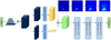 |
Fig. 7 Design of the MKMS-FPN. The network decouples spatial attention and channel attention to separately model positional saliency and semantic importance before recombining them for enhanced feature representation. Multiple convolutional kernels with different receptive field sizes are used to capture astronomical targets at different spatial scales. The receptive field visualizations illustrate how multi-kernel aggregation enlarges the perceptual range, enabling simultaneous sensitivity to compact sources and extended emission. |
3.3 Loss function design
The inherent sparsity of raw data and the extremely limited spatial extent of faint targets often lead to significant bias towards the background in the FPN and RPN modules during the ROI proposal and classification stages. The standard classification task at the ROI head is formulated as a binary decision between source and background. The baseline classification loss is the standard binary cross-entropy loss:
![Mathematical equation: \mathcal{L}_{\mathrm{CE}} = -\left[y \log(p) + (1-y)\log(1-p)\right],](/articles/aa/full_html/2026/05/aa58042-25/aa58042-25-eq1.png) (1)
(1)
where y ∈ {0,1} denotes the ground-truth label and p is the predicted source probability.
This auxiliary constraint is formulated as
 (2)
(2)
where h * x is the convolutional feature map, y is approximated using a simulated PSF sample, ui are predefined structural basis functions (morphological priors of the cross-shaped PSF), and wi are the corresponding weights. Table 1 shows that the basis set {ui} includes key spatial templates derived from the canonical cross-shaped PSF structure.
The total loss is therefore defined as
 (3)
(3)
where λ is a small weighting factor. In our experiments, we set λ = 0.1, ensuring that the cross-entropy loss remains the dominant term, while the PSF constraint acts as a weak regular-izer. This design suppresses false positives caused by structured background fluctuations, particularly in the faint-source regime, while preserving the discriminative capacity of the standard classification loss.
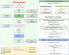 |
Fig. 8 Implementation of the MKMS-FPN backbone. Feature maps from backbone stages C2-C4 are projected and fused through top-down and lateral connections to form a multi-scale pyramid. The SPFF (spatial pyramid feature fusion) module aggregates multi-scale context using multiple pooling branches followed by convolutional fusion. The FCM (feature channel module) applies spatial and channel attention on two branches that are recombined to produce attention-weighted features. The MKPConv block performs parallel depthwise convolutions with kernel sizes {1,3,5,7} (with padding) followed by a 1 × 1 pointwise convolution to fuse multi-scale responses. The resulting pyramid features (P2-P5) are used for region proposal and detection. |
Spatial basis set for PSF morphology.
3.4 Classifier
In addition to the convolutional improvements, we enhanced the model’s detection performance by incorporating a multibranch classifier at the downstream stage. We noted that, prior to classification, photon counts were background-corrected using local estimates. The multibranch classifier (source vs. background) is designed to analyze both the rich feature maps extracted from the convolutional layers and the prior physical features derived from astronomical knowledge.
Specifically, the proposed framework consists of three independent branches: the first processes the original image data, the second handles high-dimensional convolutional feature maps extracted by a backbone network, and the third incorporates handcrafted physical priors. Each branch is designed to extract optimized representations from its respective input modality. The modular structure of the multibranch classifier is illustrated in Fig. 9.
Additionally, the specific feature definitions and computations are illustrated in Fig. 10. The 19 physical features are encoded by fully connected layers and fused with convolutional features using concatenation and attention mechanisms, yielding the final binary classification output. This design enables the model to leverage both the representational power of deep features and the domain relevance of physical parameters in a complementary manner.
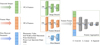 |
Fig. 9 Multibranch classifier implemented by a three-branch network with a feature fusion module. |
 |
Fig. 10 Morphological and physical feature extraction for candidate source classification. The morphological features were computed by partitioning the candidate ROI into a cross-shaped layout aligned with the instrument PSF, including the central region, the axial arms, and corner regions. These features summarize photon counts, regional means and densities, a global standard deviation, and a PSF fitting consistency score. The physical features include aperture photometry, S/N, a power-law spectral slope, and the FWHM. |
4 Results
In this section, we evaluate the proposed framework using a test dataset composed of real EP WXT observations and the augmented data generated from the real EP WXT events with known fluxes, with exposure times ranging from 1500 to 2500 s. The distribution of detection samples across different flux intervals is summarized in Fig. 11. We conduct a comparative analysis between our framework, a baseline model based on Faster R-CNN, and the widely used astronomical source detection software SExtractor. In addition, we perform ablation studies to assess the data augmentation strategy and individual network modules, and further analyze the performance of the downstream multibranch classifier in enhancing detection capability.
4.1 Overall performance and comparative analysis
As is shown in Table 2, we compared the performance of our proposed model with traditional methods and baseline models including Bayesian methods, SExtractor (Bertin & Arnouts 1996) and the two-stage Faster R-CNN baseline (Jia et al. 2023) for detecting faint sources across various flux ranges. The definitions of the precision, recall, and F1 score are given as follows:
 (4)
(4)
 (5)
(5)
and
 (6)
(6)
where
TP (true positive) refers to the number of correctly identified positive instances,
FP (false positive) refers to the number of incorrectly identified positive instances, and
FN (false negative) refers to the number of missed positive instances.
SExtractor: SExtractor, with image sizes of 256×256, achieves a relatively balanced performance in both precision and recall, demonstrating fairly good recall for lower flux ranges (flux < 1 mCrab), indicating its capability to reliably detect faint sources. Given this performance, we regard SExtractor as an effective general-purpose detection benchmark. However, despite these strengths, SExtractor’s performance improvement slows as flux increases, especially for brighter sources (flux > 1 mCrab). The growth in recall is slower compared to machine learning models. This is mainly due to SExtractor’s reliance on handcrafted features and fixed thresholds, limiting its ability to adapt to different flux conditions. As a result, SExtractor’s performance plateaus with higher-flux sources, while the framework continues to show consistent improvements.
PSF-matched filtering with Gaussian fitting: to explore the applicability of traditional X-ray astronomy tools, we implemented a two-stage approach that first convolves the image with the lobster-eye PSF matrix for matched-filter detection, then refines the candidates using a 2D Gaussian model within a maximum-likelihood fitting framework (e.g., using Sherpa (Siemiginowska et al. 2024). However, this hybrid approach achieves very low precision (0.04) and recall (0.0191 for faint sources). The performance suggests that combining a non-Gaussian PSF-matched filter with a subsequent Gaussian parametric fit may not be a suitable strategy for this data, likely because the final fitting stage cannot adequately represent the complex source morphology captured by the initial filter.
Bayesian likelihood detection with a PSF model: we further implemented a Bayesian detection method that directly incorporates the instrumental PSF matrix into a Poisson likelihood function (Cash statistic). This approach avoids Gaussian approximations and performs a pixel-wise likelihood-ratio test between source-plus-background and background-only models. This method yields better precision (0.15) and substantially higher recall for bright sources (flux > 1 mCrab) than the Gaussian-fitting approach. However, its performance remains far below that of our framework, especially for faint sources (recall = 0.017 for flux < 1 mCrab). The primary limitations are twofold: (i) in the low-count regime, faint sources often produce incomplete, irregular PSF realizations that deviate from the ideal template, reducing the likelihood even when a true source is present; and (ii) the current simplified background treatment cannot effectively distinguish between true PSF arms and structured background fluctuations, leading to spurious detections.
Baseline models: the baseline256 within the RF model offers better precision (0.81) for faint sources, but the recall is lower. The baseline512 within the RF model achieves richer features for larger sources, but the precision significantly drops to 0.50 for faint sources, showing that the larger input image size introduces noise that affects the detection performance.
Proposed framework: our framework significantly improves detection, particularly for flux < 1 mCrab, where recall reaches 0.1608, a substantial gain over SExtractor (0.0629). For flux >2 mCrab, precision is 0.9 with recall at 0.85, and for flux >3 mCrab, recall increases to 0.95. This demonstrates the effectiveness of our PSF morphology-based convolutions and multi-scale feature extraction in maintaining high precision and recall across flux ranges.
A more detailed recall analysis is shown in Fig. 12. Detecting sources with flux < 1 mCrab remains challenging due to the low S/N and high source density. Nevertheless, our framework achieves a recall of 0.18-0.22 for 0.6 mCrab < flux < 1 mCrab while sustaining a precision of 0.9, effectively doubling or tripling the number of detectable sources compared to other methods. For brighter sources, recall reaches 0.85 at flux > 2 mCrab and 0.90 at flux > 3 mCrab, ensuring high completeness for ordinary sources. When relaxing the precision constraint to 0.5, recall further increases to 0.28-0.32 for 0.6 mCrab < flux < 1 mCrab and shows a marked gain for flux < 0.6 mCrab, confirming the framework’s sensitivity to faint-source features.
Fig. 13 presents the F1 scores across flux intervals. SExtractor achieves a slightly better performance at the faint end (flux < 0.6 mCrab), where its recall contributes to higher F1 scores compared to some traditional machine learning baselines. This advantage, however, diminishes rapidly as the flux increases. With brighter sources, for which both the source brightness and the apparent size of the detection targets grow, the capacity of machine learning models to extract richer features becomes more pronounced, resulting in substantially higher F1 scores than those of SExtractor. The limited feature extraction ability of SExtractor, based on fixed thresholds, restricts its adaptability in these regimes.
In comparison, our framework consistently maintains significantly higher and more stable F1 scores across all flux intervals. This improvement arises from the morphology-aware convolution module, which enhances feature extraction, and the multi-kernel, multi-scale design, which balances detection capability across different source sizes. Moreover, by employing a multibranch downstream classifier, the framework effectively balances output precision and recall, thereby achieving a more favorable trade-off and stronger robustness under diverse flux conditions.
To better compare the detection results, we considered the significant variation in sample sizes across different flux intervals (as analyzed in Fig. 11). We then assessed the number of detected sources within different S/N intervals, using a log-scale count for clearer representation. As is shown in Fig. 14, we observe that for S/N > 10, the detection counts and trends for all methods are relatively similar, with no substantial differences. However, our framework demonstrates a clear advantage, maintaining consistently higher detection counts across the S/N range. This indicates that our framework not only detects more sources but also exhibits improved performance stability compared to the other models as S/N increases, further supporting its superiority in handling varied detection conditions.
Recall and precision by flux interval for different models.
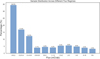 |
Fig. 11 Distribution of detection samples across different flux intervals. In the test dataset, a substantial number of sources fall into the faint regime (flux < 0.6 mCrab), where detection is particularly challenging and the demand is higher. |
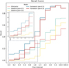 |
Fig. 12 Recall comparison across flux intervals. The proposed framework achieves markedly higher recall in the faint-source regime (flux < 1 mCrab), about two to three times that of benchmark models. For brighter sources, recall exceeds 0.85 at flux >2 mCrab and 0.90 at flux >3 mCrab, ensuring high completeness. |
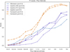 |
Fig. 13 F1 score across different flux intervals for the proposed framework, Faster R-CNN baselines, and SExtractor. |
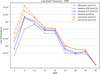 |
Fig. 14 Distribution of detected sources across S/N intervals in logscale, computed using the Li-Ma significance formula to account for imbalanced source counts in the faint (flux < 1) regime. |
4.2 Ablation analysis
To validate the effectiveness of the core module design, we designed a series of ablation experiments on the test dataset. Ablation analysis is widely used to isolate and quantify the contribution of individual components, thereby validating the effectiveness of the overall model design (LeCun et al. 2015; Zoph et al. 2018). Experimental results in Table 3 exhibit the effectiveness of all contributions in this work.
We conducted ablation experiments to assess the contributions of data augmentation, PSF-guided morphological convolution (PSFConv), and the multi-kernel multi-scale FPN (MKMS-FPN). Adding multidimensional data augmentation to the baseline CNN improved recall by 5% with flux > 1 mCrab, confirming its role in enriching feature diversity. PSFConv delivered the largest gains, improving recall by up to 13% over the baseline, highlighting its effectiveness in extracting PSF-aligned morphological features. MKMS-FPN provided moderate improvements (3-4%), mainly by balancing multi-scale feature representations and mitigating target occlusion. Even without data augmentation, the full framework improved recall by 5% (flux < 1 mCrab) and 9.8% (flux > 1 mCrab), showing its robustness. Under stricter precision constraints, recall decreased due to low-S/N limitations, indicating the need for enhanced preprocessing and refined downstream classification. In summary, PSFConv drives the most substantial performance gains, with MKMS-FPN offering complementary improvements. Together, these components substantially enhance detection performance and set the stage for further improvements via downstream classification modules.
Ablation analysis of framework modules.
Comparison of precision, recall, and F1 score for different models with and without hybrid data.
4.3 Classifier performance
To evaluate the proposed multibranch architecture, we compared it against several common classifiers (light gradient boosting machine (LightGBM) (Ke et al. 2017), random forest (RF) (Breiman 2001), recurrent neural network (RNN) (Elman 1990), graph neural network (GNN) (Scarselli et al. 2008), and Transformer (Vaswani et al. 2017) using both raw and hybrid data. The results are reported in Table 4. For a more intuitive performance comparison, we also provide summarized bar plots in Fig. 15.
The results clearly demonstrate that the inclusion of hybrid features consistently enhances classifier performance across nearly all models. When using raw features alone, all classifiers exhibited limited recall and correspondingly low F1 scores (ranging from 0.26 to 0.55), indicating a high false-negative rate and an inability to fully capture astrophysical source characteristics. With the integration of hybrid features - which combine conventional physical attributes with learned representations from a convolutional backbone - LightGBM and random forest show noticeable improvements, with F1 scores rising to 0.64 and 0.67, respectively. More substantially, sequence- and attentionbased models such as RNN and Transformer display dramatic gains, with the Transformer model achieving an F1 score of 0.81. This suggests that hybrid features effectively provide structured and semantically enriched inputs that help sophisticated models leverage their representational capacity.
Notably, applying PCA-based dimensionality reduction to the hybrid features further improves the performance for certain architectures (e.g., Transformer F1 score reached 0.83), underscoring the compatibility of hybrid features with feature compression and their utility in reducing computational overhead without sacrificing critical information. All subsequent appearances should be in the acronym form (unless at the beginning of a sentence). Any acronyms that are defined in the abstract need to be re-introduced in the main text. In contrast, the GNN performance declines with hybrid features, likely due to its limited suitability for directly modeling high-dimensional convolutional features that are not naturally represented as graphs. Overall, the universally positive response of most classifiers to hybrid features underlines their role as robust and informative descriptors that mitigate the limitations of raw physical measurements or unstructured deep features alone.
The proposed multibranch architecture capitalizes on its dedicated design for multimodal feature extraction and fusion, consistently outperforming all benchmarked classifiers. By processing raw images, high-level feature maps, and engineered physical parameters through separate yet synergistic branches, the model effectively captures both salient structural patterns and critical domain-specific attributes. The subsequent fusion via attention-weighted concatenation further ensures a balanced and context-aware integration of heterogeneous features. This structured approach not only yields superior predictive performance (F1 = 0.91) but also enhances representational richness, providing a robust framework that leverages the complementary strengths of data-driven and physics-informed features in astronomical source detection.
Feature importance analysis provides a quantitative way to interpret black-box classifiers by ranking the contribution of each input feature to the prediction outcome (Breiman 2001; Lundberg & Lee 2017). In the astrophysical context, this allows us to connect machine learning predictions with physically meaningful attributes, helping to identify which descriptors drive classification decisions. As is shown in Fig. 16, photometric value emerges as the dominant factor, followed by PCA-derived components and the full width at half maximum (FWHM). Importantly, several PCA features achieve a comparable importance to classical descriptors, indicating that high-dimensional convolutional representations provide effective complementary information to prior physical attributes. This not only improves the interpretability of our hybrid framework, but also demonstrates that integrating learned features with astrophysical priors yields tangible and physically meaningful gains for source detection tasks. Overall, Fig. 16 illustrates how hybrid features bridge physical measurements and deep representations, offering both an enhanced performance and clearer interpretability.
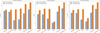 |
Fig. 15 Comparison of precision, recall, and F1 score for different models with and without hybrid data, highlighting the performance improvement of the multibranch model. |
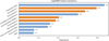 |
Fig. 16 Hybrid features integrate physical priors with learned representations to enhance interpretability and detection performance. |
5 Conclusion
This study addresses the challenge of detecting cross-shaped, low-flux sources in long-exposure lobster-eye X-ray telescope images, where conventional CNNs often struggle under low-S/N and with complex source morphology. By combining multidimensional data augmentation, PSF-guided morphological convolution (PSFConv), a multi-kernel multi-scale feature pyramid (MKMS-FPN), and a hybrid multibranch classifier, the proposed framework significantly enhances source detectability. Using simulated long-exposure WXT data and in-orbit EP observations, the framework achieves 90% precision with recall rates of 0.85 and 0.95 for sources above 2 and 3 mCrab, respectively, and more than doubles the number of detectable sources with flux < 1 mCrab compared with conventional CNNs and the SExtractor pipeline. Overall, the proposed framework provides a sensitive, efficient, and integrated end-to-end solution for multi-scale target detection.
Acknowledgements
This work is supported by and uses data from the Einstein Probe mission, a space mission under the Strategic Priority Program on Space Science of the Chinese Academy of Sciences, in collaboration with ESA, MPE, and CNES. We acknowledge the financial support from the National Natural Science Foundation of China. This work is supported by the National Natural Science Foundation of China (Grant Nos. 12433005, 12333004).
References
- Angel, J. 1979, in Space Optics Imaging X-Ray Optics Workshop, 184, SPIE, 84 [Google Scholar]
- Band, D., Matteson, J., Ford, L., et al. 1993, ApJ, 413, 281 [Google Scholar]
- Benezeth, Y., Jodoin, P.-M., Emile, B., Laurent, H., & Rosenberger, C. 2010, J. Electron. Imaging, 19, 033003 [Google Scholar]
- Bertin, E., & Arnouts, S. 1996, A&ASS, 117, 393 [Google Scholar]
- Breiman, L. 2001, Mach. Learn., 45, 5 [Google Scholar]
- Chen, Z., Wu, H., Wu, W., et al. 2025, IEEE J. Sel. Top. Appl. Earth Obs. Remote Sens., 18, 20708 [Google Scholar]
- Cheng, H., Ling, Z., Zhang, C., et al. 2024, Exp. Astron., 57, 10 [Google Scholar]
- Cheng, H., Pan, H.-W., Liu, Y., et al. 2026, A&A, in press https://doi.org/10.1051/0004-6361/202556050 [Google Scholar]
- Cheng, H., Zhang, C., Ling, Z., et al. 2025b, Exp. Astron., 60, 15 [Google Scholar]
- Cui, X., Luo, J., Deng, J., et al. 2025, ARFC-WAHNet: Adaptive Receptive Field Convolution and Wavelet-Attentive Hierarchical Network for Infrared Small Target Detection [Google Scholar]
- Elman, J. L. 1990, Cogn. Sci., 14, 179 [Google Scholar]
- Feng, W.-C., Jia, S.-M., Zhao, H.-H., et al. 2024, Study of Wide-Field-of-View X-ray Observations of the Virgo Cluster Using the Lobster Eye Imager for Astronomy [Google Scholar]
- Geological, B. 2024, Data Study Group Final Report, Tech. rep. [Google Scholar]
- Jeffs, B. D., Warnick, K. F., Landon, J., et al. 2008, IEEE J. Selected Top. Signal Process., 2, 635 [Google Scholar]
- Jia, P., Liu, W., Liu, Y., & Pan, H. 2023, ApJSS, 264, 43 [Google Scholar]
- Ke, G., Meng, Q., Finley, T., et al. 2017, Adv. Neural Inform. Process. Syst., 30 [Google Scholar]
- LeCun, Y., Bengio, Y., & Hinton, G. 2015, Nature, 521, 436 [Google Scholar]
- Ling, Z., Sun, X., Zhang, C., et al. 2023, Res. Astron. Astrophys., 23, 095007 [Google Scholar]
- Lucke, R. L., & Kessel, R. A. 2006, Opt. Eng., 45, 056403 [Google Scholar]
- Lundberg, S. M., & Lee, S.-I. 2017, Adv. Neural Inform. Process. Syst., 30 [Google Scholar]
- Nammour, F., Akhaury, U., Girard, J., et al. 2022, A&A, 663, A69 [NASA ADS] [CrossRef] [EDP Sciences] [Google Scholar]
- Preece, R. D., Briggs, M. S., Mallozzi, R. S., et al. 2000, ApJSS, 126, 19 [Google Scholar]
- Salmon, J., Harmany, Z., Deledalle, C.-A., & Willett, R. 2014, J. Math. Imaging Vis., 48, 279 [Google Scholar]
- Sawano, T., Yonetoku, D., Arimoto, M., et al. 2020, in Space Telescopes and Instrumentation 2020: Ultraviolet to Gamma Ray, 11444, SPIE, 946 [Google Scholar]
- Scarselli, F., Gori, M., Tsoi, A. C., Hagenbuchner, M., & Monfardini, G. 2008, IEEE Trans. Neural Netw., 20, 61 [Google Scholar]
- Selig, M., & Enßlin, T. A. 2015, A&A, 574, A74 [NASA ADS] [CrossRef] [EDP Sciences] [Google Scholar]
- Siemiginowska, A., Burke, D., Günther, H. M., et al. 2024, ApJSS, 274, 43 [Google Scholar]
- Sołtan, A. 2010, A&A, 532, A19 [Google Scholar]
- Van Inneman, A., Hudec, R., Pina, L., & Gorenstein, P. 1999, in X-ray Optics, Instruments, and Missions II, 3766, 72 [Google Scholar]
- Vaswani, A., Shazeer, N., Parmar, N., et al. 2017, Adv. Neural Inform. Process. Syst., 30 [Google Scholar]
- Voges, W., Aschenbach, B., Boller, T., et al. 1999, arXiv preprint [arXiv:astro-ph/9909315] [Google Scholar]
- Westerkamp, M., Eberle, V., Guardiani, M., et al. 2024, A&A, 684, A155 [NASA ADS] [CrossRef] [EDP Sciences] [Google Scholar]
- Xiao, Y., Xu, T., Xin, Y., & Li, J. 2025, Proceedings of the AAAI Conference on Artificial Intelligence, 39, 8673 [Google Scholar]
- Yang, J., Liu, S., Wu, J., et al. 2025, Pinwheel-shaped convolution and scalebased dynamic loss for infrared small target detection [Google Scholar]
- Yuan, W., Zhang, C., Feng, H., et al. 2015, arXiv e-prints [arXiv:1506.07735] [Google Scholar]
- Yuan, W., Zhang, C., Ling, Z., et al. 2018, SPIE Conf. Ser., 10699, 1069925 [Google Scholar]
- Yuan, W., Zhang, C., Chen, Y., & Ling, Z. 2022, The Einstein Probe Mission, eds. C. Bambi, & A. Santangelo (Singapore: Springer Nature Singapore), 1 [Google Scholar]
- Yuan, W., Dai, L., Feng, H., et al. 2025, Sci. China Phys. Mech. Astron., 68 [Google Scholar]
- Zhang, B., & Meszaros, P. 2004, Int. J. Mod. Phys. A, 19, 2385 [NASA ADS] [CrossRef] [Google Scholar]
- Zhang, C., Ling, Z., Sun, X., et al. 2022, ApJ, 941, L2 [Google Scholar]
- Zoph, B., Vasudevan, V., Shlens, J., & Le, Q. V. 2018, in Proceedings of the IEEE Conference on Computer Vision and Pattern Recognition, 8697 [Google Scholar]
- Zuo, X., Tao, Y., Liu, Y., et al. 2024, Res. Astron. Astrophys., 24, 085016 [Google Scholar]
All Tables
Comparison of precision, recall, and F1 score for different models with and without hybrid data.
All Figures
|
Fig. 1 Photon statistics and spectral properties of a typical brightness sample. The left panel shows the photon count distribution, with flux represented on a logarithmic scale. The middle panel presents the linear fit of the power-law spectral slope, which aligns with the theoretical expectations for gamma-ray burst spectra, though noise causes significant fluctuations. The right panel displays the spatial distribution of photon points on the detector plane, enhanced using a logarithmic scaling for better visibility. |
| In the text | |
|
Fig. 2 Data processing workflow for CNN input: raw FITS images are expanded into three channels: the original grayscale image, a photon weighted map, and a power-law spectral slope map based on photon arrival times. These are segmented into overlapping time windows, creating a sequence of frames with temporal features for CNN input. |
| In the text | |
|
Fig. 3 Detection framework architecture. Based on a Faster R-CNN backbone, the model integrates two key components: (1) PSF-guided morphological convolution for improved feature extraction, and (2) multi-scale FPN for enhanced spatial feature representation. Together, these form an integrated end-to-end pipeline for astronomical object detection. |
| In the text | |
|
Fig. 4 Feature maps and heat maps across ResNet50 bottlenecks show that increasing depth (e.g., Bottleneck4 to Bottleneck6) does not improve focus on faint cross-shaped sources. Instead, deeper layers exhibit diffuse attention and amplified noise, reducing feature distinctness. |
| In the text | |
|
Fig. 5 Wavelet-enhanced PSF-guided morphological convolution. After decomposing the input into multi-scale frequency components via wavelet transform, the model applies a cross-shaped convolutional structure that conforms to the morphology of astronomical PSFs, particularly the extended arms. This design aggregates dispersed information along the PSF pattern toward the central region, thereby enhancing weak, extended features. The receptive field visualization illustrates how this morphological structure enlarges the perception range and improves sensitivity to cross-shaped sources. |
| In the text | |
|
Fig. 6 Detailed architecture of the feature extraction backbone. The network consists of four hierarchical stages. An initial feature extraction block maps the input from 3 to 64 channels and integrates a wavelet transformer and a PSF-guided pinwheel convolution (PSFConv) to preserve multi-scale frequency information and PSF-aligned morphology. Each stage is built from residual bottleneck blocks with CBAM attention for adaptive feature refinement. The PSFConv module applies four directional convolutions (two horizontal and two vertical) followed by fusion to model the cross-shaped PSF structure of Lobster-Eye optics. The wavelet transformer decomposes features into four subbands, processes them via grouped convolution, and reconstructs the spatial representation via inverse wavelet transform, enabling frequency-aware feature enhancement before entering deeper layers. |
| In the text | |
|
Fig. 7 Design of the MKMS-FPN. The network decouples spatial attention and channel attention to separately model positional saliency and semantic importance before recombining them for enhanced feature representation. Multiple convolutional kernels with different receptive field sizes are used to capture astronomical targets at different spatial scales. The receptive field visualizations illustrate how multi-kernel aggregation enlarges the perceptual range, enabling simultaneous sensitivity to compact sources and extended emission. |
| In the text | |
|
Fig. 8 Implementation of the MKMS-FPN backbone. Feature maps from backbone stages C2-C4 are projected and fused through top-down and lateral connections to form a multi-scale pyramid. The SPFF (spatial pyramid feature fusion) module aggregates multi-scale context using multiple pooling branches followed by convolutional fusion. The FCM (feature channel module) applies spatial and channel attention on two branches that are recombined to produce attention-weighted features. The MKPConv block performs parallel depthwise convolutions with kernel sizes {1,3,5,7} (with padding) followed by a 1 × 1 pointwise convolution to fuse multi-scale responses. The resulting pyramid features (P2-P5) are used for region proposal and detection. |
| In the text | |
|
Fig. 9 Multibranch classifier implemented by a three-branch network with a feature fusion module. |
| In the text | |
|
Fig. 10 Morphological and physical feature extraction for candidate source classification. The morphological features were computed by partitioning the candidate ROI into a cross-shaped layout aligned with the instrument PSF, including the central region, the axial arms, and corner regions. These features summarize photon counts, regional means and densities, a global standard deviation, and a PSF fitting consistency score. The physical features include aperture photometry, S/N, a power-law spectral slope, and the FWHM. |
| In the text | |
|
Fig. 11 Distribution of detection samples across different flux intervals. In the test dataset, a substantial number of sources fall into the faint regime (flux < 0.6 mCrab), where detection is particularly challenging and the demand is higher. |
| In the text | |
|
Fig. 12 Recall comparison across flux intervals. The proposed framework achieves markedly higher recall in the faint-source regime (flux < 1 mCrab), about two to three times that of benchmark models. For brighter sources, recall exceeds 0.85 at flux >2 mCrab and 0.90 at flux >3 mCrab, ensuring high completeness. |
| In the text | |
|
Fig. 13 F1 score across different flux intervals for the proposed framework, Faster R-CNN baselines, and SExtractor. |
| In the text | |
|
Fig. 14 Distribution of detected sources across S/N intervals in logscale, computed using the Li-Ma significance formula to account for imbalanced source counts in the faint (flux < 1) regime. |
| In the text | |
|
Fig. 15 Comparison of precision, recall, and F1 score for different models with and without hybrid data, highlighting the performance improvement of the multibranch model. |
| In the text | |
|
Fig. 16 Hybrid features integrate physical priors with learned representations to enhance interpretability and detection performance. |
| In the text | |
Current usage metrics show cumulative count of Article Views (full-text article views including HTML views, PDF and ePub downloads, according to the available data) and Abstracts Views on Vision4Press platform.
Data correspond to usage on the plateform after 2015. The current usage metrics is available 48-96 hours after online publication and is updated daily on week days.
Initial download of the metrics may take a while.