


| Issue |
A&A
Volume 710, June 2026
|
|
|---|---|---|
| Article Number | A13 | |
| Number of page(s) | 12 | |
| Section | Astrophysical processes | |
| DOI | https://doi.org/10.1051/0004-6361/202556571 | |
| Published online | 28 May 2026 | |
Giant radio pulses in the magnetar XTE J1810−197 detected with the IAR’s telescopes
1
Instituto de Astronomía Teórica y Experimental, CONICET-UNC, Laprida 854, X5000BGR, Córdoba, Argentina
2
Facultad de Matemática, Astronomía, Física y Computación, UNC. Av. Medina Allende s/n, Ciudad Universitaria, CP:X5000HUA, Córdoba, Argentina
3
Instituto Argentino de Radioastronomía (CCT La Plata, CONICET; CICPBA; UNLP), C.C.5, (1894), Villa Elisa, Buenos Aires, Argentina
4
Facultad de Ciencias Astronómicas y Geofísicas, Universidad Nacional de La Plata, Paseo del Bosque, B1900FWA, La Plata, Argentina
5
Department of Space, Earth and Environment, Chalmers University of Technology, SE-412 96 Gothenburg, Sweden
6
Center for Computational Relativity and Gravitation, Rochester Institute of Technology, 85 Lomb Memorial Drive, Rochester, New York, 14623, USA
★ Corresponding author: This email address is being protected from spambots. You need JavaScript enabled to view it.
Received:
24
July
2025
Accepted:
26
February
2026
Abstract
Context. XTE J1810−197 is one of the six magnetars that exhibit radio emission, sometimes visible only during periods of increased activity or outbursts. XTE J1810−197 underwent its latest outburst in December 2018.
Aims. We analyzed the population of single pulses of XTE J1810−197 in radio, characterized its timing properties, and explored the potential connection between magnetars and fast radio bursts (FRBs).
Methods. We observed XTE J1810−197 between 29 September 2022 and 14 July 2023 with the radio telescopes at the Argentine Institute of Radioastronomy (IAR). We searched for single pulses in time series at a dispersion measure (DM) range of 100–400 pc cm−3, with a signal-to-noise ratio (S/N) threshold of 8. We folded each observation to obtain an integrated pulse profile. We also analyzed archival X-ray observations of the MAXI instrument from the same period, and studied the flux evolution and the magnetar’s activity.
Results. We found 249 giant pulses (GPs) at a DM mean value of 178.8 ± 0.1 pc cm−3. We measured peak flux densities up to 119 Jy, and fluences up to 58 Jy ms. We fitted a power-law distribution to the flux density, obtaining an index of −4.0 ± 0.3. We observed a maximum rate of approximately 15 pulses per hour on 20 February 2023, followed by an abrupt disappearance of transient radio emission, indicating a transition to a less active state. The brightest single pulses are limited to ∼2% of the rotational phase and have similar fluence values to the reported intermediate FRB-like bursts of SGR 1935+2154. No significant X-ray activity in the MAXI data was detected during the radio observing period.
Conclusions. This is the first study of single radio pulses of a magnetar using IAR data, showing the potential of the upgraded telescopes for investigating the transient radio sky. The properties of the single pulses detected here show the magnetar transient nature and capability to emit high-luminosity pulses. We compared the detected emission to FRB-like bursts and single pulses emitted by SGR 1935+2154. Even though the mechanism producing all the events should be coherent, the luminosity of the events, features on the dynamic spectra, and the difference between being phase confined or not, indicate that XTE J1810−197 presents GP emission, while SGR 1935+2154 only shows normal single pulses or FRB bursts. This could indicate that the conditions for producing each type of event differ.
Key words: methods: data analysis / methods: observational / stars: magnetars / stars: neutron / stars: individual: XTE J1810-197 / radio continuum: general
© The Authors 2026
 Open Access article, published by EDP Sciences, under the terms of the Creative Commons Attribution License (https://creativecommons.org/licenses/by/4.0), which permits unrestricted use, distribution, and reproduction in any medium, provided the original work is properly cited.
This article is published in open access under the Subscribe to Open model. This email address is being protected from spambots. You need JavaScript enabled to view it. to support open access publication.
1. Introduction
Magnetars are neutron stars with extremely strong surface magnetic fields (B ∼ 1013–1015 G). They are among the youngest and slowest neutron stars, with periods from ∼1 to 12 s (Olausen & Kaspi 2014). They display a rich transient phenomenology, including giant flares, short bursts, and outbursts, detected mainly at X-rays and γ-rays (Kaspi & Beloborodov 2017). The energy for the emission is provided by the decaying magnetic fields, which could be composed of a twisted dipole plus some local twisted multipole field (Duncan & Thompson 1992; Tong 2023).
Only 6 out of the 30 known magnetars have been detected in radio to date (Olausen & Kaspi 2014)1, five of which presented transient radio pulsations that are in general associated with X-ray outbursts. The sixth magnetar, SGR 1935+2154, has been found to emit a fast radio burst (FRB) (Bochenek et al. 2020) and FRB-like radio bursts. During its October 2022 outburst, bright radio bursts were detected within the nine-hour interval between the two glitches of an unusual double-glitch event (Maan et al. 2022a; Dong & Chime/Frb Collaboration 2022; Hu et al. 2024). This radio activity may have arisen from the emergence of a short-lived magnetospheric wind, as proposed by Hu et al. (2024). The detection of FRB 200428 from SGR 1935+2154 strongly supports the hypothesis that magnetars can power at least some FRBs. These results turned the community’s attention toward the conditions required for a magnetar to produce a FRB-like burst.
Studying the pulsed radio emission of magnetars provides an avenue to explore their unique spectral-temporal properties and phenomenology. This radio emission has been detected across a wide range of frequencies, observed as an integrated pulse profile and as bright single pulses. Furthermore, the radio emission exhibits transient episodes of activity, characterized by short-duration (e.g., daily) on-off switching that can occur even in the absence of concurrent X-ray activity, as exemplified by magnetar PSR J1622-4950 (Levin et al. 2010). It also shows high pulse-to-pulse variability in single pulses and in folded pulses (Kaspi & Beloborodov 2017; Esposito et al. 2021, for recent reviews).
XTE J1810−197 was the first magnetar detected at radio frequencies (Halpern et al. 2005; Camilo et al. 2006). Here we present the results of a timing and single-pulse analysis on the radio observations of XTE J1810−197 conducted daily with the radiotelescopes at the Argentine Institute of Radioastronomy (IAR) between September 2022 and July 2023. We also present an analysis of the X-ray activity during this period using archival observations of the Monitor of All-sky X-ray Image (MAXI). This work is the first single-pulse study of magnetar observations ever done with the IAR telescopes, and the first study of the radio activity of the magnetar in the mentioned epoch.
The structure of the paper is as follows. In Sect. 2 we review previous observational results associated with this magnetar. In Sect. 3 we describe the observations obtained in this work. In Sect. 4 we present the reduction and data analysis. In Sects. 5 and 6 we show the results obtained from the radio and X-ray observations, which we discuss in Sect. 7. We summarize our main conclusions in Sect. 8.
2. The magnetar XTE J1810−197
XTE J1810−197 was discovered serendipitously in X-rays on 15 July 2003 by the Rossi X-ray Timing Explorer (RXTE) while observing a soft gamma repeater. It had a transient X-ray outburst between 17 November 2002 and 23 January 2003. With the study of its spin-down rate and slow period (∼5.54 s), it showed the first signatures of being a magnetar (Ibrahim et al. 2004). It was the first of its class with detected radio emission, initially as a point source in 2004 interferometric observations (Halpern et al. 2005) and later via radio pulses in single-dish observations beginning in 2006, revealing its transient nature (Camilo et al. 2006). This is known in the literature as the first radio and X-ray outburst of the source.
Camilo et al. (2006) showed that the magnetar emitted bright, narrow, and highly linearly polarized pulses in each rotation, suggesting that a magnetar could have pulsar-like emission. They noted that the observed radio emission requires a coherent mechanism, which is likely powered by pair production enabled by the strong voltage induced in the magnetosphere. While the resulting radio beam may be narrow and miss our line of sight, its activation is linked to magnetospheric twisting. As reviewed by Kaspi & Beloborodov (2017), the emission is thought to originate from long-lived currents produced by the magnetosphere untwisting, along magnetic field lines in the magnetosphere far from the star. In the 2006 study they detected single pulses of width ≤10 ms and flux densities of ≤10 Jy. The period of detected radio activity went from 2004 until the end of 2008 (Camilo et al. 2016). This last study showed the extremely unpredictable behavior of the radio emission of the magnetar. The pulse profile showed day-to-day variations, changing the number of components, and the radio spectrum changed from being flat in 2004 to a steeper one by 2008. In addition, the radio emission suddenly disappeared until the 2018 outburst.
A second radio and X-ray outburst was detected in late 2018, with an onset between 26 October and 8 December 2018 in radio and between 20 and 26 November 2018 in X-rays (Lyne et al. 2018; Levin et al. 2019; Gotthelf et al. 2019). On the following days – 14, 19, and 20 December – integrated radio pulse profiles were detected with the IAR telescopes (Del Palacio et al. 2018). Several different radio studies were conducted following this outburst. The evolution of the pulse profile and the behavior of the broadband spectra and polarization were extensively studied (Dai et al. 2019; Levin et al. 2019; Eie et al. 2021; Desvignes et al. 2024; Lower et al. 2024), including observations at frequencies as low as 300 MHz (Maan et al. 2022b) and as high as 353 GHz (Torne et al. 2022). The main results obtained were that the pulse profile showed a daily changing behavior and a steeper spectrum (Torne et al. 2022).
Other studies focused on single-pulse analysis (Maan et al. 2019; Caleb et al. 2022; Bause et al. 2024). The latter two made an analysis on long-term observations and were able to analyze the change in the single-pulse population throughout the period from 8 December 2018 to 14 November 2021; Bause et al. (2024) was the one with the most recent observations. An interesting result was the detection of bursts of emission in the form of giant pulses (GPs) or GP-like events (Maan et al. 2019; Bause et al. 2024; Caleb et al. 2022) from this magnetar. Clearly, there is no universal consensus on the definition of GPs. One thing on which there is agreement is that they are extremely energetic and occur in a narrower phase window compared to normal pulses. One working definition in previous studies on XTE J1810−197 is that the pulse’s energy is ten times the average energy. Caleb et al. (2022) obtained the average pulse energy from the integrated profiles of only the rotations that did not present GP-like emission. We considered that all the detected single pulses are GPs (see Sect. 7.1). To asses the energetics of the pulses, we introduced the fluence defined as Speak × τ, where Speak is the flux density of the peak and τ is the pulse duration2.
The observations with the shortest sampling time were taken with the Effelsberg telescope, with a sampling of 131 μs (Caleb et al. 2022), followed by the Stockert telescope with 218.45 μs (Bause et al. 2024) and finally the Giant Metrewave Radio Telescope (GMRT) with 655 μs (Maan et al. 2019). This is relevant when identifying the substructure and width of the pulses.
We note that different works use slightly different definitions of a single pulse and its width depending on the method employed. Caleb et al. (2022) defines a single pulse as the emission detected within one rotation of the neutron star, sometimes presenting substructure or spiky emission, while Bause et al. (2024) defines a single pulse as the spiky emission, where several single pulses could occur in one rotation. Bause et al. (2024) found pulse widths in the range of 0.65–30 ms; around 50% of the pulses had a width of ≤4 ms. The flux densities they found ranged from just a 1–3 Jy to up to 300 Jy, with some outliers of 600 Jy.
Interestingly, the average fluxes in radio and X-rays are not correlated, as shown by Caleb et al. (2022) during May–September 2020 and by Bause et al. (2024) during February 2021. This suggests that the activity in the radio regime may evolve independently of the X-ray activity.
3. Observations
3.1. Radio observations
We performed high-cadence observations of XTE J1810−197 with the two 30 m single-dish antennas at IAR, Carlos M. Varsavsky (A1) and Esteban Bajaja (A2), located in Parque Pereyra Iraola, Argentina (Gancio et al. 2020). The monitoring started on 29 September 2022 (MJD 59851) and continued until 14 July 2023 (MJD 60139). Although it was close to the ecliptic in December, we note that the source was never behind the Moon or the Sun.
Each antenna’s receiver consists of two Ettus boards. For A1, the central frequency was 1424 MHz with a bandwidth of 112 MHz divided into 128 channels, on one circular polarization. In the case of A2, the central observing frequency was set to 1428 MHz with a bandwidth of 56 MHz divided into 64 channels, on both circular polarizations. The sample time in both cases was 146 μs. The data was recorded into filterbank files. Here we analyzed 149 days of observations obtained with A2. The A1 observations were excluded from the analysis due to a higher level of radio-frequency interferences (RFIs). The A2 observing times ranged between 18 min and 172 min, yielding a total of 269 h on source. We highlight that this high-cadence campaign covered approximately 52% of the observing period.
The geographic location of the IAR provides unique access to temporal windows unavailable to other radio telescopes during previous high-cadence campaigns. Figure 1 compares the possible hours on source for several telescopes (Parkes, GMRT, Stockert, Effelsberg), considering their elevation limit. As it is a southern source, IAR can observe XTE J1810−197 for almost 13 hours above the horizon, although mechanical limitations reduce its maximum tracking time to 3.6 h. Figure 1 shows that high-cadence campaigns with several telescopes enable the detection of intraday transient events, highlighting the benefit of geographically dispersed observations.
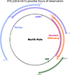 |
Fig. 1. Observable time of XTE J1810−197 for different telescopes that have conducted high-cadence campaigns. The arc matching the telescope’s color represents the source’s possible observation time for that telescope. We highlight the very short overlap between the IAR and other observatories. |
In mid-2022 the IAR underwent an upgrade with the installation of a parallel digitalizer board consisting of Reconfigurable Open Architecture Computing Hardware (ROACH) boards. Virtually, the IAR antennas have two receivers that differ only on the digitalizer board, either Ettus or ROACH. In August 2022, we started the calibration of the system employing the ROACH board, calibrating the noise diode MC7014 ENR 35dB (Araujo Furlan et al. 2023). The efforts on the calibration of the dual-polarization of A2 can be found in Gancio et al. (2024). We only have a noise temperature value for the ROACH board.
The flux density values obtained in this work rely on two main assumptions. First, the noise temperature was identical for both the Ettus and the ROACH board, and second, the noise temperature remained constant throughout the entire observation period. These assumptions are justified below.
Equation (1) describes the noise temperature for a receiver
 (1)
(1)
where TN is the total noise temperature for a receiver composed of f elements. The parameters TN1 and G1 are the individual noise temperature and gain of the first element, respectively, TN2 and G2 of the second element, and so on. The contribution of the final element is minimal as it is divided by the product of the gains of all preceding stages. Consequently, the first element in the receiver chain dominates the overall noise temperature. In our case, the final element was the digitalizer board, either the ROACH or the Ettus. The two boards received the same input signal. Their noise temperature contribution was insignificant as the factor that multiplies them is on the order of 10−6.
Since we only have systematic measurements of the noise temperature from mid-2023, covering nearly a year of daily data (from June 2023 to May 2024), we adopted the average value measured during this period: TN = 50 ± 8 K. The receiver system underwent no modifications during this time, thus supporting the assumption of stability. We therefore consider this value representative of the system from September 2022 to May 2024, with any potential variation reflected in the quoted uncertainty.
Thus, we obtained the flux density of a temporally resolved single pulse using the modified radiometer equation (e.g., Maan & Aswathappa 2014)
 (2)
(2)
where Tsys is the system temperature in K, Ae(z) is the effective collecting area as a function of the zenith angle (0.3 times the area of the 30m dish for A2 in m2), Δν is the bandwidth in Hz (56 × 106 Hz), np is the number of polarizations (2 for A2), (S/N)peak is the peak signal-to-noise ratio of the pulse, and W the observed pulse width. In this work, we consider Tsys as the noise temperature of the system. After cleaning for RFIs, we determined that one or two channels were fully masked in all observations, and used Δν as 0.9 of the observed bandwidth (0.9 × 56 × 106 Hz).
3.2. X-ray observations
We analyzed archival X-ray observations of XTE J1810−197 to search for possible correlations with the radio emission. We studied the daily light curves of XTE J1810−197 provided by the MAXI instrument (Matsuoka et al. 2009). MAXI is a high-energy astrophysical experiment on board the International Space Station (ISS). It comprises two semicircular arc-shaped X-ray slit cameras with a wide field of view (FoV). It harbors two kinds of X-ray detectors that collect photons from the slit cameras: a gas proportional counter, the Gas Slit Camera (GSC; working in the 2–30 keV band), and an X-ray CCD, the Solid-state Slit Camera (SSC; operating in the 0.5–12 keV range). MAXI maps the entire sky on each orbit of the ISS, every ∼92 min.
The data that MAXI provides are already processed with different time binning. We used the one-orbit light curves, and associated ∼15° FoV images, together with the all-sky maps to check possible source contamination3. The observations retrieved spanned the period from 1 September 2022 (MJD 59823) to 28 April 2024 (MJD 60428).
4. Reduction and data analysis
4.1. Radio
The radio analysis involves two main parts. The first part was carried out by the PuMA pipeline4, which employs PRESTO (Ransom 2011) as its core tool and uses it to perform RFI masking and phase folding of the observations. This is described in detail in Section 4.1.1. The second part, focused on transient activity, was performed with a bash pipeline developed for this work, described in Section 4.1.2. After processing all observations with these pipelines, we conducted an in-depth analysis with a Python-based script.
4.1.1. Timing
We used the RFIFIND and PREPFOLD tasks in the PRESTO package to remove RFIs and fold the entire duration of each observation using a previously reported ephemeris to obtain integrated pulse profiles. Next, we used the task PAT in PSRCHIVE (Hotan et al. 2004; van Straten et al. 2012) to calculate the time of arrival (TOA) using the Fourier phase gradient-matching method for template fitting. We used the pulse profile of an observation with high S/N to construct the template with the PSRSMOOTH package in PSRCHIVE.
We developed a timing model to characterize the rotation of the magnetar by tracking the TOAs of its pulses. We used a Taylor expansion to describe the temporal evolution of the pulsar phase
 (3)
(3)
where ν,  , and
, and  represent the rotation frequency of the magnetar and its first and second derivatives at the reference epoch t0, and φ is the phase of the pulsar at t0. Various physical phenomena, such as glitches or sudden changes in the frequency derivative can be investigated through this method (Antonopoulou et al. 2022).
We first obtained the parameters for the timing model from Camilo et al. (2016), and subsequently updated them by fitting our data to the timing model (Eq. (3)) using the TEMPO2 software package (Hobbs et al. 2006).
To address jitter and systematic errors, we incorporated the parameters EFAC and EQUAD. These parameters model white noise by adjusting each TOA uncertainty as
 (4)
(4)
where σi represents the TOA uncertainty for each observation derived from the cross-correlation between the template profile and the folded observation. EFAC accounts for the unmodeled instrumental effects and inaccuracies in TOA uncertainty estimates, while EQUAD addresses additional sources of time-independent uncertainties, such as pulse jitter.
We used TempoNest (Lentati et al. 2014) to determine EFAC and EQUAD once we fitted the rotational parameters of the magnetar, maintaining the solution fixed and considering a small data span to discard red noise effects, as described in Zubieta et al. (2023).
4.1.2. Single pulses
We studied the transient activity searching for single pulses. For this we employed the PRESTO PREPSUBBAND task to dedisperse the data. This produces a dedispersed temporal series at a dispersion measure (DM) value specified beforehand. We searched for single pulses between a DM range of 100–500 pc cm−3, with incremental steps of 1 pc cm−3. We did not use the parameter ZERODM to help discard RFIs, as it produced artifacts on our time series that did not contribute to RFI classification. We searched each dedispersed time series for single pulses with PRESTO SINGLE_PULSE_SEARCH.PY script. We chose a threshold value of S/N > = 8 (Maan et al. 2022b) and the remaining parameters on default, searching for pulses in a downsampling range of 2–30, or pulse width of 0.293–4.389 ms.
We found that setting a threshold as high as S/N ≥ 8 was restrictive enough, as visual inspection of the diagnostics plots and the pulses themselves mainly revealed pulses from the magnetar. This is illustrated in a diagnostic plot from SINGLE_PULSE_SEARCH.PY in Fig. 2, for 19 November 2022. The detected pulses appeared clustered around a DM of 178 pc cm−3.
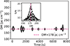 |
Fig. 2. Single-pulse search carried out with PRESTO on 19 November 2022 for the DM range. Time = 0 corresponds to the start of the observation. Each circle represents a pulse detected with a S/N ≥ 8; its size is proportional to its S/N. The dashed horizontal line marks the DM of the magnetar (178 pc cm−3). The pulses align in elongated islands centered around the magnetar DM. Pulses that are farther from that line (e.g., at ∼6200 s) are more likely to be RFIs. Inset: Distribution of pulse S/N as a function of DM. The pink vertical line marks the DM of the magnetar. The distribution of the pulses’ S/N is also centered at the magnetar DM. |
We extracted the candidates from all the searches and analyzed them with a Python-based script. Each circle in Fig. 2 represents a possible identified signal, hereafter referred to as an event. A pulse is defined as a collection of events produced by the detection of a pulse across different time series (i.e., at varying DM values). To avoid multiple detections of the same pulse, we assumed that events at different DM values coinciding within a millisecond were produced by the same pulse. This millisecond threshold served as an initial empirical criterion, justified by the following: (1) the neutron star rotational period of ∼5.54 s implies that two pulses coincident to the millisecond should come from the same rotation, and (2) the widths of single pulses previously reported span a few milliseconds (Caleb et al. 2022; Bause et al. 2024). For each pulse, the DM value was taken from the highest S/N event within the group. This way, each group of circles depicted in Fig. 2 was considered a single pulse if it met our criteria.
Additionally, since previous studies estimated the DM of the magnetar within a range of 178–180 pc cm−3, we restricted our selection to pulses with DM values between 170–190 pc cm−3, resulting in a subset of 419 candidate pulses. This set included misclassified RFIs, duplicates, and real astrophysical pulses. We identified 249 single pulses through visual inspection of the diagnostic plots, as shown in Fig. 2. The following step was to match the 249 visually identified pulses with the 419 candidates and to obtain a clean definitive sample.
First, we fitted a Gaussian profile to each candidate. We defined the pulse width as the full width at half maximum (FWHM),  , with σ obtained from the fit. This parameter allowed a simple identification and RFI removal as poorly fitted Gaussians produced outlier widths in the distribution. We manually cross-checked the remaining pulses, using both the diagnostic plots and the fitted profiles, and we discarded any remaining duplicates. High S/N pulses often appeared in several more time series than lower S/N ones. Due to our coincidence criterion –based on truncating event times to the nearest millisecond– some events from the same pulse were assigned slightly different timestamps, thus resulting in false duplication. For instance, a pulse occurring at 567.479956 s and extending across several DMs could result in some events being truncated to 567.479 s and others to 567.480 s, hence producing two identifications for the same pulse. In such cases, we checked whether the pulse centers were consistent and examined the S/N versus DM distribution of all events within ±0.5 s of the center (∼1/5 of a period). Figure 3 shows an example of a duplicated pulse. Through visual inspection of the time series, we confirmed the duplicates and assigned the correct DM based on the S/N peak. This process allowed us to reconstruct the properties of all 249 visually identified pulses.
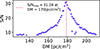 |
Fig. 3. S/N vs DM distribution of one pulse detected on 25 November 2022, at time 7128.940 s from the start of the observation. It appeared at two different times: 7128.939 s and 7128.940 s. It was detected in 75 different time series across a DM range of 127–210 pc cm−3, peaking in S/N at DM = 179 pc cm−3. |
4.2. MAXI X-ray data
We restricted our study of the light curve from the MAXI data to the MJD range 59850–60428. We extended the analysis beyond the date range in radio after observing a peak in the light curve that recurred with a one-year interval. Following consultations with the MAXI team, we had to distinguish whether the minor activity observed in the magnetar light curve was intrinsic to the source or was the result of contamination from the Sun or a nearby source.
MAXI discards the observations of a source when it is close in the sky to the Sun within a certain angular distance. As the Sun was in an active phase within its 12-year activity cycle, contamination of the light curves due to solar leakage was still possible. The contamination can appear due to scattering of solar photons, mainly in the 2–4 keV band. Hence, a possible confusion arises as the magnetar activity is mostly seen in soft X-rays. The MAXI team kindly performed an on-demand removal of solar contamination from the data. We worked with the cleaned light curves of XTE J1810−197 in both the 2–20 keV and the 4–20 keV energy bands. The difference between those light curves represents the activity in the 2–4 keV range. We cross-checked the light curves, the source region image, and the all-sky images available5 to see the daily variations and possible sources of contamination. In the all-sky images, the scatter from the Sun appeared as red diffuse halos originating from the point where the Sun is located.
Another potential contamination in the source light curves could be caused by nearby X-ray sources, primarily GX 9+1 and GX 13+1. Due to their small angular distance to XTE J1810−197, there was a chance that the observed variability could have originated from the intrinsic variability of such neighboring X-ray binaries. The MAXI team decontaminated the light curves by extending the neighboring source regions to reduce contamination. Additionally, if the elongated point spread function (PSF) of the MAXI instrument experienced any distortion or change in its position angle, this could also produce contamination. We examined the light curves of GX 9+1 and GX 13+1 simultaneously with the light curves of the magnetar. For the days on which observations of the magnetar and the other sources were available, we computed the correlation of the X-ray flux in the 2–20 keV band. We used the corr method in the pandas library and calculated the Pearson correlation coefficient. Finally, we analyzed the presence of the magnetar emission and the PSFs of both GX sources in the images, considering a FoV of ∼15°, combined with the variations in the light curve. In section 6 we explore in detail when contamination could be ruled out and when it could not.
5. Radio results
5.1. Timing analysis
We monitored the pulsar from 29 September 2022 (MJD 59851) to 14 July 2023 (MJD 60140). However, we only detected the folded profile until 10 January 2023 (MJD 59954). Within this date range, we performed 60 observations of the magnetar and detected it 16 times.
To obtain the timing solution for these observations, we fitted ν,  , and
, and  to the TOAs, keeping DM fixed at 178 pc cm−3 (Caleb et al. 2022). The results are shown in Table 1 and the residuals for the model are shown in Fig. 4. We obtained a phase-coherent solution between MJD 59851 and MJD 59954. After this epoch, we were not able to detect the folded profile of the magnetar. This reduction in the activity of the pulsar agrees with the reduction in the activity of GPs.
Results for the timing model by fitting to the TOAs analyzed in this work.
5.2. Single pulses
5.2.1. Transient activity
Over 149 days of observations, we detected single pulses in 56 days. In the remaining 93 days we were not able to detect pulses with our criteria.
The final sample consists of 249 single pulses from the magnetar. We analyzed the transient activity in terms of the rate, i.e., the number of pulses per hour. To obtain the rate, we determined the effective observing time tobserved for each observation by taking the total exposure time and excluding intervals in which more than 70% of the frequency channels were masked.
We assumed the emission process to be Poissonian, and we assigned to the number of pulses from a day, Nday, an uncertainty of  . Finally, we calculated the rate as Nday/tobserved. For non-detection days, we estimated an upper limit as 1/tobserved indicating that < 1 single pulses were detected on those days, following the method of Lazarus et al. (2012). Since the observation durations ranged from 18 min to 172 min, shorter observations on non-detection days resulted in higher upper limits.
The resulting rate is shown in Fig. 5. In the upper panel we show the rate considering all the single pulses. A peak in activity occurred on 20 January 2023, after which only two days had detected single pulses. This suggests that the magnetar experienced a highly active state before its radio emission dropped below the sensitivity limit of the IAR telescopes. In the lower panel we present the rate only considering pulses with S/N ≥ 15 in order to highlight the behavior of the most energetic pulses. In this case the upper limit represents the non-detection of pulses with S/N ≥ 15. This decomposition reveals that the rate of more energetic pulses was higher earlier in the campaign, even though the overall peak in activity occurred shortly before the subsequent decline. We computed the minimum detectable flux density of single pulses with the next relation (e.g., Pastor-Marazuela et al. (2023))
 (5)
(5)
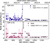 |
Fig. 5. Rate of pulses per hour of observation against days of observation. The upper panel shows the rate considering only pulses of S/N ≥ 8 and the lower panel only of S/N ≥ 15. The circles represent the rates and the filled triangles are the upper limits. |
where G (in K/Jy) is the telescope gain, β ∼ 1 the digitization factor for the IAR, tobs the observation time, and W the width considered. The remaining values are the same from Equation 1. In general, when there is no detection, a broad value of W is used, such as 10 ms. In this case we considered a value of 4.4 ms as it was the broader width in our search. The result is upper limits for flux density and luminosity respectively of Smin = 7 ± 1 Jy and Lmin = 600 ± 100 Jy pc2 for a single pulse.
5.2.2. Pulses properties
We analyzed the distribution of the width of the pulses (FWHM), flux density, and the fluence (or energy) of all the single pulses. We considered that all of our single pulses are GPs (see Section 7.1).
We fitted the FWHM distribution using curvefit from scipy with two different models. One consisted of a lognormal plus a Gaussian distribution (L+G) and the other consisted of two lognormal functions (L+L). The upper panel of Fig. 6 displays the resulting distributions overlaid on the data. There is a principal component in the range of 0.2–0.7 ms, and a second component for higher FWHM. In Table 2, the resulting parameters are shown, along with the χred2 and the number of degrees of freedom (d.o.f.). The L+G model is favored, with a χred2 = 0.78 against a value of 1.42.
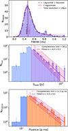 |
Fig. 6. Histograms of pulses grouped by different properties, together with the best fit of the distribution. Upper Panel: FWHM distribution fitted with L+G (black dotted) and L+L (pink continuous curve) models. The vertical lines show the time resolution (gray), the exp(μ1) value of the lognormal component of the L+G model (black), and the exp(μ1) value of the first lognormal component of the L+L model (pink). Middle and lower panels: Flux density and fluence distributions with the respective completeness limit indicated by vertical dotted lines. The sloped line indicates the fit and the shadowed area the uncertainty range. |
Parameters for the fitted models of the FWHM.
Previous studies of the flux density distribution of the pulses from the magnetar have modeled it as a power-law function (Maan et al. 2019) or a broken power law (Caleb et al. 2022). To study our distribution, we applied a flux density threshold at 30 Jy, at the transition of the peak of the distribution; this limit is consistent with the lower bound of the power law obtained in the fit (the parameter x min). We studied the distributions in two ways. First, we studied NSpeak, the number of pulses detected in a 5.5 Jy flux density interval, using a Knuth binning in the linear space. We assume the emission process is Poissonian and assign error bars as the square root of the number of pulses in each bin. We employed CURVE_FIT from SCIPY, which uses a nonlinear least squares fitting of our model, a power law  . The optimized value obtained was α = −4.0 ± 0.3. In the middle panel of Fig. 6, we show our full sample and indicate the completeness limit. We plot the distribution on a logarithmic scale, where the power-law behavior is represented with straight lines. The different colored bins represent which bins were used for the fitting and which were ignored.
The second method comprised a power-law fit to the flux density’s probability density function (PDF). We used the Python package POWERLAW (Alstott et al. 2014) to obtain the power-law index (α) that best fits the data. This method employs Pareto’s maximum likelihood estimate (MLE) to determine the optimal index. It gives the minimum flux density value (x min) to adjust the power law by finding the minimal Kolmogorov-Smirnov distances between the fitted power law and the data. In this case, it was 30.18 Jy, which is our completeness threshold. We obtained the uncertainty of α by performing a bootstrap with replacement 1000 times. We obtained α = −4.1 ± 0.4 for the distribution. Since both fitted values agree, we used the first method’s value; the corresponding fit appears in the middle panel of Fig. 6.
For the fluence, we applied the same methodology as for the flux density. We considered a fluence completeness limit of 12.5 Jy ms, obtained empirically and confirmed with POWERLAW. In this case, we studied the number of pulses NFluence in a 2.9 Jy ms interval. The index of the fitted power law with SCIPY was α = −3.0 ± 0.2 and with POWERLAWα = −3.3 ± 0.5. As before, we considered the value from the first method.
Figure 7 presents the time evolution of both the FWHM and the flux density. The FWHM appears to decrease and stabilize over time. The vertical line marks the day with the highest rate of detected single pulses, coinciding with one of the brightest single pulses with Sν = 118 ± 19 Jy. The brightest pulse was detected on 10 January 2022 (MJD 59954), with a flux density of 119 ± 19 Jy, while the faintest detected pulse occurred with Sν = 16 ± 3 Jy on 24 October 2022. Following this peak activity – marked by both the highest pulse rate and brightest pulses – the magnetar’s activity diminished substantially, becoming virtually undetectable for the IAR sensitivity.
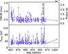 |
Fig. 7. FWHM and flux density variation through the days. In the lower panel the dotted horizontal line is the flux density completeness limit. |
5.2.3. Morphology, DM, phase, and periodicity
The sample of single pulses shows no particular behavior on their dynamic spectrum. In Fig. 8 we dedispersed the brightest pulse on 20 January 2023, at 179 pc cm−3. The diminished central band intensity aligns with the known frequency response characteristic of our receiver.
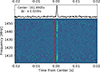 |
Fig. 8. Dynamic spectrum (lower) and time series (upper) for the brightest pulse of 20 January 2023, dedispersed at 179 pc cm−3. The center of the time series (161.6905 s) represents the time from the start of the observation. The vertical red line is shown for reference and corresponds to a pulse of DM = 179 pc cm−3. |
As previously mentioned, the pulses had a range of possible DM values. When producing plots as shown in Fig. 8, we confirmed the astrophysical origin of the pulses. Our DM resolution, based on our sample time, was approximately 0.93 pc cm−3. Technically, our uncertainty in each measured DM is of 1 pc cm−3. However, by analyzing the pulses distribution, we can statistically narrow down the magnetar DM. We fitted a Gaussian distribution to the number of pulses per DM (upper panel of Fig. 9). The parameters were μ = 178.8 ± 0.1 pc cm−3, σ = 1.15 ± 0.09 pc cm−3, with a χred2 = 2.26 and six d.o.f.
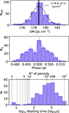 |
Fig. 9. Upper panel: Distribution of the pulse DM. The dash-dotted line is the Gaussian fit, the vertical line is μ, and the colored area represents the uncertainty of the value. Middle panel: Distribution of pulse phases. Lower panel: Distribution of log10 of the waiting time between two consecutive pulses. The vertical lines indicate waiting times equal to multiples of the spin period. |
We studied the dispersion in the phase of all our GPs, as shown in the middle panel of Fig. 9. For each date, we calculated the period with our timing solution and assumed it was constant throughout the observation. The maximum phase difference for pulses within the same observation was Δφ = 0.0196, which represents approximately 2% of the magnetar’s rotational period. Since we had days with detected GPs but not an integrated pulse profile, this prevented us from consistently aligning the GPs based on a timing solution. Thus, we aligned the mean phase of each day by manually shifting each to 0.5, and applied the same shift to each individual phase. The maximum difference in shifted phases across all observations was Δφ = 0.0239, which represents approximately 2.4% of the neutron star’s rotational period. Our results indicate that the detected emission originates from roughly 2.4% of the magnetar’s rotational phase. This small phase range corresponds to an observed opening angle of the emission region of 8.64°. We found no correlation between pulse phase and brightness (Sν), with Pearson and Spearman correlation coefficients of 0.03 and 0.02, respectively.
We analyzed the waiting-time distribution between consecutive single pulses to determine the typical interval required for subsequent pulse detection. The lower panel of Fig. 9 displays this distribution in both logarithmic units (log10(waiting time)) and in units of magnetar rotation periods. We only observed one case of two consecutive rotations with GPs detected. The waiting time shows a main distribution center at around 100–208 periods and a secondary minimum between 1 and 3 periods. A waiting time shorter than one period would indicate multiple peaks in one single rotation, i.e., the detection of substructure. The observed distribution is evidence of the non-detection of substructure in our observations. The mean waiting time is 562.7 s (101 periods) with a standard deviation of 3.7 s (0.7 periods).
Previous studies of this magnetar have shown that single pulses and giant micro pulses are emitted across a wide range of rotational phases, generally coinciding with the window of the integrated pulse profile (Kramer et al. 2007; Serylak et al. 2009; Dai et al. 2019; Maan et al. 2019; Bause et al. 2024). In contrast, GPs appears at a limited phase range (Serylak et al. 2009; Caleb et al. 2022), with GPs from the 2003 outburst limited to ∼4° (Serylak et al. 2009) and for the 2018 in a range of ∼9 − 10°, either preceding or lagging behind the folded profile (Caleb et al. 2022). Figure 10 displays the 16 integrated pulse profiles and their corresponding single-pulse phase range, indicated by vertical dotted lines. For pre-November 2022 observations, the single-pulse phase range aligns with the peak of the noisy integrated profile. From November onward, we observe a trailing phase drift in some observations, most notably in the profile from 6 November 2022. Of the 16 days with detected profiles, only one lacked detection of single pulses. On all the other days where both integrated pulse profiles and GPs were detected, there was at least one GP with S/N ≥10, including two days with only one GP detected (S/N = 13 and 28). Of 78 days with GPs but without profiles, many exhibit pulses with S/N ≥10, particularly the bright GP on 20 January 2023 (S/N = 40, Sν = 118 ± 19 Jy).
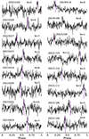 |
Fig. 10. Integrated pulse profiles for the days with detection. For each day, the number of single pulses detected is indicated by N. Vertical lines indicate the mean phase (in pink) along with the minimum and maximum pulse phase values (in violet) for individual pulses. |
These results align with prior studies (Serylak et al. 2009; Caleb et al. 2022; Bause et al. 2024), suggesting the emission comprises two distinct components: a normal (steady) component and a GP component. On the days with detected profiles, the profile phase width is wider than the single-pulse phase range. This difference may arise from the underlying normal component or from single pulses below our instrumental sensitivity. This is shown by days of non-alignment between the profile peaks and single-pulse phase range, and by one profile detection without corresponding single pulses.
6. X-ray results: MAXI
We examined the magnetar’s light curve to check whether the detected peaks at around 0.1-0.2 c/s/cm2 at 2–20 keV were produced by its activity or is due to contamination. The peaks that recurred with a one-year interval disappeared in the Sun-cleaned data. However, some smaller peaks persisted on other days. We paid particular attention to three date ranges, namely 29 September to 9 December 2022 (MJD 59851–59922), 2 January to 5 June 2023 (MJD 59946–60100), and 13 September to 4 December 2023(MJD 60200–60282), as these periods exhibited increases in the measured flux. We found that some days appeared to be contaminated by diffuse scattering from the Sun, but not all.
When we analyzed the light curves of the GX sources, they did not exhibit the same behavior as XTE J1810−197. The Pearson correlation coefficient indicated no correlation between their fluxes with that of the magnetar, with values of −0.12 for GX 9+1 and 0.14 for GX 13+1. Although these values suggest a lack of correlation, further examination of the PSF distortion revealed that the peaks observed in the light curve of the magnetar tended to occur when the PSFs of the other sources were elongated and aligned with the position of the magnetar. The shape and orientation of the PSFs varied from day to day, affecting or producing the peaks detected in the magnetar light curve.
We found that all variations in the X-ray light curves can be attributed either to contamination from the Sun or to a distorted PSF from neighboring bright sources. On some days, both sources of contamination were present. The magnetar itself did not exhibit any detectable activity during this period in the data collected by the MAXI instrument.
7. Discussion
7.1. Giant pulses
Our sample consists exclusively of GPs. However, as we have mentioned, there is no universal consensus about how a GP should be defined. Various studies adopt different criteria. Some define a GP when its energy exceeds ten times the average energy of all single pulses; others use a similar characterization but invoke flux density; and yet others classify a pulse as a GP if its flux density is ten times the average peak flux density of the folded profile6. In previous studies of this magnetar, Caleb et al. (2022) reported GPs with peak flux densities up to 158 mJy. In this work, we detected pulses with flux densities from 16 ± 3 Jy up to 119 ± 19 Jy, i.e., up to three orders of magnitude higher in peak flux density. Based on this comparison, we consider that the entire sample of pulses consists only of GPs. This type of criterion appears in literature – especially in studies with the Crab pulsar, for instance Karuppusamy et al. (2010), Doskoch et al. (2024) – where a pulse is considered a GP if its S/N exceeds a certain threshold.
Another criterion often used to identify GPs is the study of the flux and fluence distribution. Typically, GPs describe a power-law distribution, in contrast with the normal or lognormal distributions of normal pulsar emission. We performed this analysis on the IAR data and fitted a power-law distribution to the flux density and fluence of the pulses, supporting the GP classification. Additional evidence comes from the narrow phase range reported, especially when compared to the broader apparent phase width of the integrated profiles in Fig. 10.
A comparison of the flux density and fluence distributions with other works is as follows. For the previous outburst, Serylak et al. (2009) reported a power-law index of −1.85 for the energy distribution of GP at higher frequencies (8.5 GHz). Our results indicate a steeper energy distribution for the 2018 outburst. Caleb et al. (2022) reported a broken power law for the flux density with a power of about −1 or −4, depending on the flux density range. Maan et al. (2019) found that the high-energy tails of the distribution, where the brightest pulses showed similarities to GPs, were described by a simple power law with a mean index of ∼ − 3.3 across five observations. Bause et al. (2024) noted that their single pulses did not follow a power law, possibly due to the different definition used for a single pulse. Following the behavior observed in the previous outburst, where pulse energy distributions changed daily, our sample might indicate an evolution between the epoch studied by Bause et al. (2024) and our observations.
We fitted a single power law of index α = −4.0 ± 0.3 to the flux density distribution, and α = −3 ± 0.2 to the fluence distribution. It is important to note that the flux density range and the epoch at which each study derived these indices differ; there is no overlap in the flux density intervals, as shown in Fig. 11. This work corresponds to the highest flux density range. The differing values could indicate a dependence on the Sν range considered or the employed bandwidth, as Maan et al. (2019) observed at lower frequencies, but primarily reflect the evolving nature of the emission. Previous studies on GPs for the Crab pulsar found a power law index of about −3 for its flux density distribution (Karuppusamy et al. 2010); the index obtained for this work is steeper.
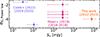 |
Fig. 11. Power-law index fitted by different studies for GPs and giant micro pulses after the 2018 outburst, color-coded by the reference and with the observation years indicated between brackets. |
7.2. Some implications of our observations
Following its outburst, the magnetar entered a period of mild transient activity in December 2018. Two subsequent peaks in radio activity were observed before our campaign –one in September 2020 and another in February 2021. The September 2020 peak marked the onset of a more sustained active phase (Caleb et al. 2022; Bause et al. 2024). The IAR observations began in September 2022 and revealed enhanced activity by February 2023, followed by a sharp decline below our sensitivity limit. This suggests that the peak in radio emission is significantly delayed with respect to the initial X-ray outburst.
Previous efforts to identify a correlation between X-ray and radio activity yielded no results. Caleb et al. (2022) reported no X-ray enhancement accompanying the radio activity. They even found an X-ray flux minimum coinciding with the rise in average radio flux density toward September 2020. Similarly, Bause et al. (2024) found no associated X-ray activity in archival Swift/XRT data from August 2020 and February–April 2021. In our analysis, we found no reportable activity on the magnetar from the MAXI observations.
The measured widths are the narrowest reported to date. We note two caveats regarding observed pulse width comparisons. First, the different methods employed make a direct comparison difficult. Second, our flux density sensitivity of Smin = 7 ± 1 Jy (for S/N = 8) means that a more sensitive telescope would likely measure wider FWHM values for the same pulses. While previous studies have detected pulses several orders of magnitude fainter, our faintest pulse is 16 ± 3 Jy. This empirical detection threshold is higher than the theoretical sensitivity calculated for the Ettus boards in Section 5.2.1. This suggests we are likely detecting only the brightest portion of each pulse. If the pulses follow a Gaussian profile, we would primarily observe the narrow peak region, explaining the small measured widths.
For a resolved single pulse with a known width (Δt), the size of the emission region can be estimated using the light travel time as r < cΔt (Lorimer & Kramer 2004), where c is the speed of light. Considering the average FWHM measured in this study, 0.469 ± 0.008 ms, we estimate a size of the emitting region of 141 ± 2 km. If the intrinsic width is broader (e.g., 1–10 ms), as reported in previous studies at similar frequencies, the corresponding size would increase to ∼300–3000 km. In any case, the radiation seems to be produced well within the magnetosphere as the radius of the light cylinder of XTE J1810-197 is ≈2.65 × 1010 cm.
The single-pulse luminosities range from (6 ± 2)×1030 erg s−1 to (5 ± 2)×1031 erg s−1, with an average value of (1.5 ± 0.7)×1031 erg s−1, approximately 10−2 times lower than the magnetar’s spin-down luminosity of 4.6 × 1033 erg s−1, as derived from our timing solution and previously reported Bsurf values. The brightness temperatures range from (3 ± 2)×1025 K to (5 ± 2)×1026 K, with a mean value of (5 ± 3)×1026 K, about a factor of 10−6 lower than the value reported for FRB20200426 (Bochenek et al. 2020) at a similar central frequency. All these temperatures, however, are well above the Compton limit of 1012 K, indicating that the radiation must be coherent.
7.3. Possibility of observing an FRB from this source
An important question about this source is whether it could present a similar behavior to SGR 1935+2154 and emit a future FRB. To get a clue, we compared the detected pulses to the radio emission from SGR 1935+2154.
The energy distributions of GPs from neutron stars and repeating FRBs share a common property as both are expected to follow a power law. As mentioned in Sect. 5.2.2, we fitted a power law to the single-pulse properties, with fluences ranging from 9 ± 3 Jy ms to 58 ± 10 Jy ms. If, as discussed earlier, the intrinsic widths of the pulses are broader, the fluence values will increase. The measured fluences overlap with the faintest values reported in Kirsten et al. (2021) for two bright radio bursts from SGR 1935+2154, neither those bursts nor the detected GPs in this work show distinct features in their dynamic spectra. The bursts reported by Kirsten et al. (2021) differ from our brightest pulses by two orders of magnitude in their specific luminosities; their waiting time was a fraction of the rotational period, and the bursts appeared at random phases, distinguishing them even from FRB20200428, which occurred in opposition to the pulsar-like emission (Zhu et al. 2023). In contrast, we detected pulses at different rotations, but within a limited phase range, marking their GP nature.
Our fluence values are comparable to two bursts reported on 8 October 2020 in Giri et al. (2023), (34.1 ± 8.1) Jy ms and (5.9 ± 1.7) Jy ms, which exhibit features in their dynamic spectra and show no phase preference (Zhu et al. 2023). The pulsar-like emission reported by Zhu et al. (2023) shows no evidence of a GP emission at those observing epochs. Their average spectral luminosity is (6.2 ± 0.2)×1029 erg s−1, which is 10−5 times the spin down luminosity, in contrast to our value of 10−2 times. The absence of GP emission, but the presence of FRB-like bursts from SGR 1935+2154 marks a difference in the phenomenology observed from this source with XTE J1810−197. XTE J1810−197 has shown to be a proficient GP emitter; in contrast, SGR 1935+2154 has shown high-energy pulses only in the form of FRB and FRB-like. It remains uncertain whether SGR 1935+2154 could emit GPs similar to XTE J1810−197 or if GPs from XTE J1810−197 could extend to higher luminosities.
In Fig. 12 we compare the reported single pulses with those of previous works of XTE J1810−197 and SGR J1935+2154. We adapted the transient phase space plot from Nimmo et al. (2022), included the reported pulses from Zhu et al. (2023) assuming a distance of 9.5 ± 2.9 kpc, and adopted a distance of 2.5 ± 0.5 kpc for XTE J1810−197 (Ding et al. 2020). Several points arise from this comparison: (1) our brightest single pulses overlap in specific luminosity/4π with the faintest radio bursts reported by Giri et al. (2023); (2) we detected some of the most luminous pulses from XTE J1810−197, consistent with the bright pulses reported by Bause et al. (2024); (3) SGR 1935+2154 exhibits standard radio single-pulse emission and bright bursts, but almost no intermediate pulses, whereas XTE J1810−197 single pulses span through a broad range of specific luminosities; (4) all the detected pulses from XTE J1810−197 to date lie below the diagonal line corresponding to a constant brightness temperature of 1027 K.
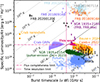 |
Fig. 12. Transient phase space adapted from Nimmo et al. (2022) including the GPs detected in this work and their error bars, previous works on XTE J1810−197 (Caleb et al. 2022; Bause et al. 2024), and a recent work on FAST radio pulses from SGR J1935+2154 (Zhu et al. 2023). In the case of SGR 1935+2154, the vertical error bar of each pulse includes the uncertainty in the magnetar distance. The pink horizontal dotted line represents our flux completeness limit, and the vertical line our time resolution limit. |
Studies suggest a twist and un-twist effect on the magnetosphere following the outburst. Borghese et al. (2021) reported that the delayed increase in the spin-down was consistent with a steady growth of a small twist. Later, Desvignes et al. (2024) argued that the observed decrease in both spin-down and width of single radio pulses pointed to a gradual untwisting of the magnetic field. Combining the geometrical interpretations from both studies, it appears that our line of sight is close to the region on the neutron star’s surface responsible for the X-ray emission, which is also the hemisphere from which the radio pulsar emission seems to originate. This interpretation is supported by the small lag between the X-ray and radio peak reported in Borghese et al. (2021). This scenario is different from the geometry proposed in Zhu et al. (2023) for SGR J1935+2154, where the radio pulsar emission and the X-ray peak were in opposition, while FRB 20200428 appeared coincidental with the X-ray peak.
Our study presents that the radio emission from magnetar XTE J1810−197 shows similarities to some intermediate bursts from SGR 1935+2154, but also important differences, making a direct extrapolation of the possibility of XTE J1810−197 to emit a FRB-like burst difficult. While reviewing this manuscript, a recent work making an in-depth analysis of this possibility has also appeared (Lal et al. 2026)7.
8. Summary and conclusions
We presented the first analysis of XTE J1810−197 observations made with the radio telescopes of the IAR, opening a new line of research for the observatory. We performed a high-cadence campaign during a time window not previously explored, starting four years after the magnetar’s latest outburst in 2018. We characterized the emission of GPs during this period and investigated possible X-ray activity.
We detected a total of 249 GPs over 149 days of observations. The 249 GPs were concentrated in 56 out of the 149 observations. We found pulses with flux densities from 16 ± 3 Jy up to 119 ± 19 Jy, centered at a DM = 178.8 ± 0.1 pc cm−3. The broad flux density range and the daily fluctuations in the rate of detected pulses highlight the extreme variability in the radio emission from the magnetar.
The GPs we detected share similar specific luminosities with some intermediate bursts from SGR 1935+2154 reported by Giri et al. (2023). However, key differences exist with FRB-like pulses from SGR 1935+2154: the bursts reported by Giri et al. (2023) are not restricted in phase, whereas our detections show a GP phase alignment, confined to a narrow rotational window. This contrasts with FRB and FRB-like emission detected from SGR 1935+2154, which either appeared in opposition to the pulsar-like component or at random phases (Zhu et al. 2023).
We found that the rate of pulses peaked on 20 January 2023, followed by a sudden drop in the emission of GPs, suggesting a transition from a high-activity state to a lower one. This behavior is coincident with that reported in Bause et al. (2024), where a sudden change in the activity of the magnetar was detected in September 2020 and another in February 2021. This may imply transitions of the magnetar between different emission states, undergoing a highly active state for two years between February 2021 and February 2023, at which the magnetar’s emission fell below our sensitivity.
Finally, we analyzed public archival X-ray observations of the magnetar from MAXI. We did not detect any X-ray activity throughout the entire observation period.
Acknowledgments
We thank the Referee for their constructive comments, which have significantly improved the quality of this work. We are grateful to the authorities and technical staff of the IAR for their continuous efforts that enable our high-cadence observational campaign. This research has made use of the MAXI data provided by RIKEN, JAXA and the MAXI team. S.B.A.F. especially thanks M. Tatehiro for the support provided when analyzing MAXI’s data. S.B.A.F. also thanks M. Lower for providing an initial ephemeris for XTE J1810-197, and M. Bause for the enriching email exchange. S.B.A.F. and E.Z. are PhD candidates with CONICET fellowships. G.E.R. and F.G. acknowledge financial support from the State Agency for Research of the Spanish Ministry of Science and Innovation under grant PID2022-136828NB-C41/AEI/10.13039/501100011033/, and by “ERDF A way of making Europe”, by the “European Union”. G.E.R. also thanks the support from PIP 0554 (CONICET). G.E.R and F.G. are CONICET researcher. F.G. acknowledges support from PIBAA 1275 and PIP 0113 (CONICET). S.d.P. acknowledges support from ERC Advanced Grant 789410. COL gratefully acknowledges support from NSF award AST-2319326, PHY-2207920 and PHY-2513442.
References
- Alstott, J., Bullmore, E., & Plenz, D. 2014, PLOS ONE, 9, e85777 [Google Scholar]
- Antonopoulou, D., Haskell, B., & Espinoza, C. M. 2022, Rep. Prog. Phys., 85, 126901 [NASA ADS] [CrossRef] [Google Scholar]
- Araujo Furlan, S. B., Gancio, G., Galante, C. A., & Romero, G. E. 2023, Boletin de la Asociacion Argentina de Astronomia La Plata Argentina, 64, 304 [Google Scholar]
- Bause, M. L., Herrmann, W., & Spitler, L. G. 2024, A&A, 686, A144 [NASA ADS] [CrossRef] [EDP Sciences] [Google Scholar]
- Bochenek, C. D., Ravi, V., Belov, K. V., et al. 2020, Nature, 587, 59 [NASA ADS] [CrossRef] [Google Scholar]
- Borghese, A., Rea, N., Turolla, R., et al. 2021, MNRAS, 504, 5244 [NASA ADS] [CrossRef] [Google Scholar]
- Caleb, M., Rajwade, K., Desvignes, G., et al. 2022, MNRAS, 510, 1996 [Google Scholar]
- Camilo, F., Ransom, S. M., Halpern, J. P., et al. 2006, Nature, 442, 892 [NASA ADS] [CrossRef] [Google Scholar]
- Camilo, F., Ransom, S. M., Halpern, J. P., et al. 2016, ApJ, 820, 110 [NASA ADS] [CrossRef] [Google Scholar]
- Dong, F. A., & Chime/Frb Collaboration 2022, ATel, 15681, 1 [NASA ADS] [Google Scholar]
- Dai, S., Lower, M. E., Bailes, M., et al. 2019, ApJ, 874, L14 [NASA ADS] [CrossRef] [Google Scholar]
- Del Palacio, S., Garcia, F., Combi, L., et al. 2018, ATel, 12323, 1 [Google Scholar]
- Desvignes, G., Weltevrede, P., Gao, Y., et al. 2024, Nat. Astron., 8, 617 [Google Scholar]
- Ding, H., Deller, A. T., Lower, M. E., et al. 2020, MNRAS, 498, 3736 [NASA ADS] [CrossRef] [Google Scholar]
- Doskoch, G. M., Basuroski, A., Halley, K., et al. 2024, ApJ, 973, 87 [Google Scholar]
- Duncan, R. C., & Thompson, C. 1992, ApJ, 392, L9 [Google Scholar]
- Eie, S., Terasawa, T., Akahori, T., et al. 2021, PASJ, 73, 1563 [Google Scholar]
- Esposito, P., Rea, N., & Israel, G. L. 2021, in Magnetars: A Short Review and Some Sparse Considerations, eds. T. M. Belloni, M. Méndez, & C. Zhang (Berlin, Heidelberg: Springer, Berlin Heidelberg), 97 [Google Scholar]
- Gancio, G., Lousto, C. O., Combi, L., et al. 2020, A&A, 633, A84 [NASA ADS] [CrossRef] [EDP Sciences] [Google Scholar]
- Gancio, G., Romero, G. E., Astudillo, J., Saavedra, E. A., & Combi, J. A. 2024, Rev. Mex. Astron. Astrofis. Conf. Ser., 56, 131 [Google Scholar]
- Giri, U., Andersen, B. C., Chawla, P., et al. 2023, arXiv e-prints [arXiv:2310.16932] [Google Scholar]
- Gotthelf, E. V., Halpern, J. P., Alford, J. A. J., et al. 2019, ApJ, 874, L25 [Google Scholar]
- Halpern, J. P., Gotthelf, E. V., Becker, R. H., Helfand, D. J., & White, R. L. 2005, ApJ, 632, L29 [NASA ADS] [CrossRef] [Google Scholar]
- Hobbs, G. B., Edwards, R. T., & Manchester, R. N. 2006, MNRAS, 369, 655 [Google Scholar]
- Hotan, A. W., van Straten, W., & Manchester, R. N. 2004, PASA, 21, 302 [Google Scholar]
- Hu, C.-P., Narita, T., Enoto, T., et al. 2024, Nature, 626, 500 [Google Scholar]
- Ibrahim, A. I., Markwardt, C. B., Swank, J. H., et al. 2004, ApJ, 609, L21 [CrossRef] [Google Scholar]
- Karuppusamy, R., Stappers, B. W., & van Straten, W. 2010, A&A, 515, A36 [NASA ADS] [CrossRef] [EDP Sciences] [Google Scholar]
- Kaspi, V. M., & Beloborodov, A. M. 2017, ARA&A, 55, 261 [Google Scholar]
- Kirsten, F., Snelders, M. P., Jenkins, M., et al. 2021, Nat. Astron., 5, 414 [Google Scholar]
- Kramer, M., Stappers, B. W., Jessner, A., Lyne, A. G., & Jordan, C. A. 2007, MNRAS, 377, 107 [Google Scholar]
- Kuzmin, A. D. 2006, Chin. J. Astron. Astrophys. Suppl., 6, 34 [Google Scholar]
- Lal, B., Maan, Y., Abdelmaguid, M., et al. 2026, ApJ, 998, 99 [Google Scholar]
- Lazarus, P., Kaspi, V. M., Champion, D. J., Hessels, J. W. T., & Dib, R. 2012, ApJ, 744, 97 [NASA ADS] [CrossRef] [Google Scholar]
- Lentati, L., Alexander, P., Hobson, M. P., et al. 2014, MNRAS, 437, 3004 [NASA ADS] [CrossRef] [Google Scholar]
- Levin, L., Bailes, M., Bates, S., et al. 2010, ApJ, 721, L33 [Google Scholar]
- Levin, L., Lyne, A. G., Desvignes, G., et al. 2019, MNRAS, 488, 5251 [Google Scholar]
- Lorimer, D. R., & Kramer, M. 2004, Handbook of Pulsar Astronomy, 4 (Cambridge, UK: Cambridge University Press) [Google Scholar]
- Lower, M. E., Johnston, S., Lyutikov, M., et al. 2024, Nat. Astron., 8, 606 [Google Scholar]
- Lyne, A., Levin, L., Stappers, B., et al. 2018, ATel, 12284, 1 [NASA ADS] [Google Scholar]
- Maan, Y., & Aswathappa, H. A. 2014, MNRAS, 445, 3221 [Google Scholar]
- Maan, Y., Joshi, B. C., Surnis, M. P., Bagchi, M., & Manoharan, P. K. 2019, ApJ, 882, L9 [Google Scholar]
- Maan, Y., Leeuwen, J. V., Straal, S., & Pastor-Marazuela, I. 2022a, ATel, 15697, 1 [NASA ADS] [Google Scholar]
- Maan, Y., Surnis, M. P., Chandra Joshi, B., & Bagchi, M. 2022b, ApJ, 931, 67 [NASA ADS] [CrossRef] [Google Scholar]
- Matsuoka, M., Kawasaki, K., Ueno, S., et al. 2009, PASJ, 61, 999 [Google Scholar]
- Nimmo, K., Hessels, J. W. T., Kirsten, F., et al. 2022, Nat. Astron., 6, 393 [NASA ADS] [CrossRef] [Google Scholar]
- Olausen, S. A., & Kaspi, V. M. 2014, ApJS, 212, 6 [Google Scholar]
- Pastor-Marazuela, I., Straal, S. M., van Leeuwen, J., & Kondratiev, V. I. 2023, A&A, 672, A151 [NASA ADS] [CrossRef] [EDP Sciences] [Google Scholar]
- Ransom, S. 2011, PRESTO: PulsaR Exploration and Search TOolkit, Astrophysics Source Code Library [record ascl:1107.017] [Google Scholar]
- Serylak, M., Stappers, B. W., Weltevrede, P., et al. 2009, MNRAS, 394, 295 [Google Scholar]
- Tong, H. 2023, arXiv e-prints [arXiv:2309.05181] [Google Scholar]
- Torne, P., Bell, G. S., Bintley, D., et al. 2022, ApJ, 925, L17 [NASA ADS] [CrossRef] [Google Scholar]
- van Straten, W., Demorest, P., & Oslowski, S. 2012, Astron. Res. Technol., 9, 237 [NASA ADS] [Google Scholar]
- Zhu, W., Xu, H., Zhou, D., et al. 2023, Sci. Adv., 9, eadf6198 [NASA ADS] [CrossRef] [Google Scholar]
- Zubieta, E., Missel, R., Sosa Fiscella, V., et al. 2023, MNRAS, 521, 4504 [Google Scholar]
This quantity is also referred as the energy of the pulse in some works on GPs (Kuzmin 2006; Karuppusamy et al. 2010).
The adoption of the number ten in these definitions suggests it is a community-adopted threshold for distinguishing between populations.
We emphasize the complementary role of observing from the IAR. While that recent work reports observations with the Green Bank Telescope (GBT) (which shares a common visibility window of this magnetar with the IAR), none are reported between MJD 59896 and 60058 (162 days). During this period, we conducted 84 observations, detecting GPs in 35. The peak activity (MJD 59969) occurred during this GBT observational gap, reinforcing the importance of high-cadence IAR observations, as the events reported here are unique and would otherwise have gone undetected.
All Tables
All Figures
|
Fig. 1. Observable time of XTE J1810−197 for different telescopes that have conducted high-cadence campaigns. The arc matching the telescope’s color represents the source’s possible observation time for that telescope. We highlight the very short overlap between the IAR and other observatories. |
| In the text | |
|
Fig. 2. Single-pulse search carried out with PRESTO on 19 November 2022 for the DM range. Time = 0 corresponds to the start of the observation. Each circle represents a pulse detected with a S/N ≥ 8; its size is proportional to its S/N. The dashed horizontal line marks the DM of the magnetar (178 pc cm−3). The pulses align in elongated islands centered around the magnetar DM. Pulses that are farther from that line (e.g., at ∼6200 s) are more likely to be RFIs. Inset: Distribution of pulse S/N as a function of DM. The pink vertical line marks the DM of the magnetar. The distribution of the pulses’ S/N is also centered at the magnetar DM. |
| In the text | |
|
Fig. 3. S/N vs DM distribution of one pulse detected on 25 November 2022, at time 7128.940 s from the start of the observation. It appeared at two different times: 7128.939 s and 7128.940 s. It was detected in 75 different time series across a DM range of 127–210 pc cm−3, peaking in S/N at DM = 179 pc cm−3. |
| In the text | |
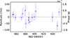 |
Fig. 4. Residuals with respect to the timing model presented in Table 1. |
| In the text | |
|
Fig. 5. Rate of pulses per hour of observation against days of observation. The upper panel shows the rate considering only pulses of S/N ≥ 8 and the lower panel only of S/N ≥ 15. The circles represent the rates and the filled triangles are the upper limits. |
| In the text | |
|
Fig. 6. Histograms of pulses grouped by different properties, together with the best fit of the distribution. Upper Panel: FWHM distribution fitted with L+G (black dotted) and L+L (pink continuous curve) models. The vertical lines show the time resolution (gray), the exp(μ1) value of the lognormal component of the L+G model (black), and the exp(μ1) value of the first lognormal component of the L+L model (pink). Middle and lower panels: Flux density and fluence distributions with the respective completeness limit indicated by vertical dotted lines. The sloped line indicates the fit and the shadowed area the uncertainty range. |
| In the text | |
|
Fig. 7. FWHM and flux density variation through the days. In the lower panel the dotted horizontal line is the flux density completeness limit. |
| In the text | |
|
Fig. 8. Dynamic spectrum (lower) and time series (upper) for the brightest pulse of 20 January 2023, dedispersed at 179 pc cm−3. The center of the time series (161.6905 s) represents the time from the start of the observation. The vertical red line is shown for reference and corresponds to a pulse of DM = 179 pc cm−3. |
| In the text | |
|
Fig. 9. Upper panel: Distribution of the pulse DM. The dash-dotted line is the Gaussian fit, the vertical line is μ, and the colored area represents the uncertainty of the value. Middle panel: Distribution of pulse phases. Lower panel: Distribution of log10 of the waiting time between two consecutive pulses. The vertical lines indicate waiting times equal to multiples of the spin period. |
| In the text | |
|
Fig. 10. Integrated pulse profiles for the days with detection. For each day, the number of single pulses detected is indicated by N. Vertical lines indicate the mean phase (in pink) along with the minimum and maximum pulse phase values (in violet) for individual pulses. |
| In the text | |
|
Fig. 11. Power-law index fitted by different studies for GPs and giant micro pulses after the 2018 outburst, color-coded by the reference and with the observation years indicated between brackets. |
| In the text | |
|
Fig. 12. Transient phase space adapted from Nimmo et al. (2022) including the GPs detected in this work and their error bars, previous works on XTE J1810−197 (Caleb et al. 2022; Bause et al. 2024), and a recent work on FAST radio pulses from SGR J1935+2154 (Zhu et al. 2023). In the case of SGR 1935+2154, the vertical error bar of each pulse includes the uncertainty in the magnetar distance. The pink horizontal dotted line represents our flux completeness limit, and the vertical line our time resolution limit. |
| In the text | |
Current usage metrics show cumulative count of Article Views (full-text article views including HTML views, PDF and ePub downloads, according to the available data) and Abstracts Views on Vision4Press platform.
Data correspond to usage on the plateform after 2015. The current usage metrics is available 48-96 hours after online publication and is updated daily on week days.
Initial download of the metrics may take a while.