| Issue |
A&A
Volume 708, April 2026
|
|
|---|---|---|
| Article Number | A321 | |
| Number of page(s) | 15 | |
| Section | Astrophysical processes | |
| DOI | https://doi.org/10.1051/0004-6361/202557296 | |
| Published online | 21 April 2026 | |
Searching for radio emission from radio quiet magnetars with MeerKAT
Max-Planck-Institut für Radioastronomie, Auf dem Hügel 69, 53121 Bonn, Germany
★ Corresponding author: This email address is being protected from spambots. You need JavaScript enabled to view it.
Received:
17
September
2025
Accepted:
28
February
2026
Abstract
Context. Magnetars are neutron stars that occupy the extreme end of the neutron star population, with magnetic field strengths greater than 1012 G. They have been proposed as one of the most likely progenitor models for the phenomenon of energetic, millisecond-duration, extragalactic radio bursts (FRBs), which have been increased even further due to the FRB-like bursts emitted from the galactic Magnetar SGR 1935+2154. However, only a low fraction of the magnetars (six in total) have been detected in the radio regime, and thus most magnetars are radio quiet.
Aims. We conducted regular observations of 13 radio quiet magnetars to probe the long-term radio quietness using the most sensitive telescope in the southern hemisphere: MeerKAT. These observations provide deep constraints on the radio emission of magnetars, relevant for the progenitor models of FRBs.
Methods. Given that MeerKAT is an interferometer, we probe the magnetars for radio emission in both the imaging and time domain. We search in the time domain in the DM range of 20 pc/cm3 10 000 pc/cm3 for single pulses using a TransientX-based search pipeline (the FRB perspective), as well as from a pulsar perspective by folding the data using the X-ray ephemeris. On the other hand, we use the imaging domain to search for persistent radio emission in total intensity and circular polarisation, as well as to create light curves using snapshot imaging, which also has a long transient perspective.
Results. We find no radio emission in the time domain for any of the observed magnetars. Nevertheless, we are providing deep limits of the mean flux density (52 μJy to 68 μJy) and the single pulse fluence 39 mJy ms to 52 mJy ms. From the image domain, we provide individual upper limits on the persistent radio emission and the light curve for the 13 magnetars. Additionally, an ultra-long period transient and an additional magnetar happened to be in the imaging beam, for which we provide lower limits as well.
Conclusions. We provide an extensive series of deep upper limits in the time domain, but also as novelty limits from the imaging domain for magnetars. As the current magnetar radio emission models are based on a few radio loud magnetars, we encourage monitoring of radio quiet magnetars independent of their X-ray flux with high cadence for further insights into their potential for emitting in the radio regime.
Key words: stars: magnetars / stars: neutron
© The Authors 2026
 Open Access article, published by EDP Sciences, under the terms of the Creative Commons Attribution License (https://creativecommons.org/licenses/by/4.0), which permits unrestricted use, distribution, and reproduction in any medium, provided the original work is properly cited.
This article is published in open access under the Subscribe to Open model.
Open access funding provided by Max Planck Society.
1. Introduction
Magnetars are a subclass of neutron stars whose inferred dipole magnetic field strengths are the highest seen in neutron stars (1012 G 1015 G). The term was originally introduced by Duncan & Thompson (1992) and Thompson & Duncan (1993) as a unified model of soft gamma-ray repeaters (SGRs) and anomalous X-ray pulsars (AXPs). The two main observable characteristic behaviours of magnetars are strong and frequent glitches and the high-energy emission in the X-ray (and partially also gamma-ray). Glitches are sudden jumps in the spin period of the neutron star, which seem to be related to the interior of the neutron star as discussed by Anderson & Itoh (1975). High-energy emission consists of a persistent profile of pulsed emission with periods in the order of 2 s to 12 s, as well as transient emission in the form of bursts and rare (giant) flare events Kaspi & Beloborodov (2017). The bursts are often clustered in time, but not necessarily periodic (GöǧüŞ et al. 1999), and are on millisecond to second scale in duration. Additionally, magnetars can undergo outbursts, in which the X-ray flux increases by a factor of 10–1000 and shows enhanced bursting activity in contrast to the quiescent state. Thus, classifying a newly found neutron star, which is not showing the hallmark observables, as a magnetar can be challenging, as only an inferred high magnetic field and the pulsed (X-ray) emission can be observed. However, the nature of transient X-ray emission is highly time variable and can change on timescales of weeks. The magnetar catalogue1 (Olausen & Kaspi 2014) includes currently 30 magnetars and magnetar candidates.
Of these magnetars, six have been observed in radio: SGR 1935+2154 (for example Bochenek et al. 2020; CHIME/FRB Collaboration 2020), XTE J1810-197 (for example Halpern et al. 2005), Swift J1818.0-1607 (for example Karuppusamy et al. 2020), SGR J1745-2900 (for example Shannon & Johnston 2013), PSR J1622-4950 (for example Levin et al. 2010), and 1E 1547.0-5408 (for example Camilo et al. 2007). The radio emission can show as short millisecond-scale radio pulses (which we refer to as single pulses in this work), of which there can be multiple in a single rotation, as well as pulsed emission at the rotational period of the magnetar, often displayed as a pulse profile. However, the appearance of the profiles, as well as the single pulses, varies with time and can show sudden changes. In XTE J1810-197, for example, as seen among others by Levin et al. (2019) and Bause et al. (2024), the number of components and the brightness of the single pulses vary over time. Additionally, the radio emission itself appears and disappears on a timescale of months to a few years (Camilo et al. 2016). Although radio emission is typically assumed to follow after an outburst of a magnetar, Caleb et al. (2022) and Bause et al. (2024) have shown that the radio flux densities for the magnetar XTE J1810-197 can increase without a corresponding increase in X-ray emission (mid 2020 and early 2021). This indicates that the paradigm of searching for radio emission only after an X-ray outburst could be biased, and hence motivates a monitoring campaign at radio wavelengths.
From the theory side, there are attempts to constrain the parameters under which magnetars are capable of emitting in the radio regime. If we assume that the radio emission mechanism of magnetars, which is not well understood, follows conditions similar to those of the emission mechanism of radio pulsars (that is, a polar cap model), we can define the so-called death line(s) of the spin period and its derivative, under which the magnetic field is too strong and thus quenches the radio emission, as shown by Chen & Ruderman (1993). Depending on the configuration of the magnetic field assumed for the death line, several radio quiet magnetars lie in the region where radio emission is expected, while radio loud magnetars lie below the death line. Hence, these alone do not suffice to predict radio emission from a magnetar. Figure 1 shows the spin period and the derivative of each magnetar considered in this work, as well as the radio loud magnetars. Also shown are the two extreme cases for the death lines, one for the case of a dipolar magnetic field configuration (higher up in Fig. 1) and for a twisted magnetic field configuration (lower in Fig. 1). Clearly, several radio quiet magnetars such as SGR 1627+41 are in the regime, where radio emission would be expected.
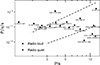 |
Fig. 1. So-called P-Pdot diagram, which shows spin period (P) vs spin period derivative (Ṗ) for the radio loud (triangles) and the radio quiet magnetars considered in this work (circles). The values are taken from from Olausen & Kaspi (2014). Additionally, two death lines are shown: simple dipolar field magnetic field (upper line) and a twisted magnetosphere (bottom line). The area in between is referred to as the death valley. |
Additionally, the so-called fundamental plane proposed by Rea et al. (2012b) is another (observational) approach to explain why only specific magnetars show radio emission by comparing the quiescent X-ray luminosity (LX) and the spin down luminosity LR (energy that is available from the spin down of the neutron star). The fundamental plane is defined as the electric potential gap as a function of LX = LR and splits the magnetars into those where the spin-down dominates (LR > LX), and those where the X-ray emission dominates (LX > LR). Based on this, Rea et al. (2012b) argue that in the case of the spin-down-dominated magnetars, a pulsar-like polar cap radio emitting process could be sustained and hence produce the radio emission. However, those with a higher LX will not show radio emission as the processes that lead to radio emission are quenched.
The clearly radio loud magnetar XTE J1810-197 challenges both of these predictions. It is centrally in the death valley (the area in between the death line for a simple dipolar magnetic field and a complex magnetic field), indicating a more complex magnetic field structure. Additionally, its X-ray luminosity exceeds the spin down luminosity, indicating that it should not emit radio emission but instead is still radio loud.
Previous searches for radio emission typically targeted the source(s) sparsely or even just once after an X-ray outburst. This includes, for example, Lorimer & Xilouris (2000) for SGR 1900+14, while Burgay et al. (2006) and Crawford et al. (2007) targeted four magnetars with one Parkes observation each. Lazarus et al. (2012) conducted a first campaign targeting several targets in the search for radio emission, focusing on a target after an X-ray outburst with the Green Bank Telescope (GBT). Even the Five-hundred-meter Aperture Spherical Telescope (FAST) has been used for searches in the radio emission of individual magnetars by Lu et al. (2024), Bai et al. (2025), and Xie et al. (2025).
Recently, magnetars have become the most actively followed progenitor models for fast radio bursts (FRBs), which are millisecond-duration extragalactic radio bursts of unknown origin. The FRB-like burst, in terms of energy and morphology, from the Galactic Magnetar SGR 1935+2154 has provided a direct observational link to FRBs (Bochenek et al. 2020 and CHIME/FRB Collaboration 2020). Later, this magnetar has been seen to emit sporadic single pulses (Kirsten et al. 2021) and faint pulsar-like states (Zhu et al. 2023). In the pulsar-like phase, several weak radio pulses from a duty-cycle were visible.
However, our understanding of the conditions under which magnetars can emit radio emission is poor. Therefore, gaining a better understanding will also give crucial insight into their eligibility to produce FRBs. Thus, we conducted regular monitoring of twelve of the radio quiet magnetars, as well as SGR 1935+2154 on a monthly basis with the MeerKAT telescope, which is a radio interferometer consisting of 64 dishes located in the Karoo semi-desert in South Africa, which has the unique ability to collect beam-forming and continuum data simultaneously. Its high sensitivity and isolated location allow us to find even the weakest emission and provide deep limits in the case of a non-detection in both the time and imaging domain presented in this work. This article is structured as follows: Sect. 2 describes the targets and observations, Sect. 3 describes our data reduction techniques, Sect. 4 presents our results, and Sect. 5 and Sect. 6 relate our findings to other works and summarise this work, respectively.‘
2. Observational strategy
2.1. Targets
From the list of magnetars that are published in the Magnetar catalogue (Olausen & Kaspi 2014), we selected those that are visible by MeerKAT and within our Galaxy. Furthermore, we also removed those only classified as magnetar candidates and those that had previously detected radio emission, with the exception of SGR 1935+2154, given its important role as a potential link to FRBs. Hence, the following 13 magnetars, listed in Table 1, were observed in our campaign.
Overview of the sources and their observing epochs.
2.1.1. 1E 1048.1-5937
Magnetar 1E 1048.1-5937 was discovered by Seward et al. (1986) in an X-ray survey with the high-energy Astronomy Observatory 2 (Einstein Observatory) in 1979. Since its discovery, the magnetar has been active with several outbursts, flux enhancements, and glitches (see Archibald et al. (2020) and references therein). An infrared counterpart has been detected by Wang & Chakrabarty (2002) for this magnetar, which is also associated with a stellar wind bubble (Gaensler et al. 2005b). Previous searches for radio emission after outbursts have not revealed radio emission (Camilo & Reynolds 2007).
2.1.2. 1E 1841-045
Vasisht & Gotthelf (1997) reported the detection of magnetar 1E 1841-045, which is associated with the supernova remnant Kes 73 with observations of the Advanced Satellite for Cosmology and Astrophysics, as an anomalous X-ray pulsar (AXP). Since its discovery, the magnetar has shown several periods of outbursts (Gavriil et al. 2002), a behaviour that is known for soft gamma ray repeaters (SGRs). Thus, AXPs and SGRs were now observationally connected under the term magnetar. Additionally, this source went into an outburst during our observational campaign, as reported in Younes et al. (2025).
2.1.3. 1RXS J170849.0-400910
The first detection of 1RXS J170849.0-400910 was reported by Voges et al. (1999) in a ROSAT All-Sky Survey (RASS) with pulsations found by Sugizaki et al. (1997). Despite flaring activity reported by Younes et al. (2020), the magnetar has relatively stable X-ray flux levels (Dib & Kaspi 2014), as well as several glitches observed (Scholz et al. 2014). However, a potential infrared counterpart (Durant & van Kerkwijk 2006) and an upper limit in mid-infrared (Wang et al. 2007) have been found. This IR emission is potentially related to the interaction between the dust and the X-ray emission, and this magnetar has only been clearly detected at high energies so far.
2.1.4. 3XMM J185246.6+003317
Zhou et al. (2014) and Rea et al. (2014) independently discovered 3XMM J185246.6+003317 using data from the X-ray Multi-Mirror Mission (XMM-Newton). Despite the X-ray emission, no low energy counterpart has been found. This only recently discovered magnetar has a comparably low magnetic field strength for magnetars (< 4 × 10¹³ G). Nevertheless, its change in spectrum and X-ray flux density classify it as a (transient) magnetar in a post-outburst stage.
2.1.5. CXOU J164710.2-455216
CXOU J164710.2-455216 was discovered as a magnetar by Muno et al. (2006) within the Westerlund I cluster with the Chandra X-ray telescope. As is common for magnetars, it showed several outbursts (Woods et al. 2011; Borghese et al. 2019). Similarly to 3XMM J185246.6+003317, this source is a magnetar with a rather low magnetic field of about 4 × 10¹³ G estimated by the timing solution of An & Archibald (2019). A potential IR counterpart has been found by (Testa et al. 2018) for this magnetar.
2.1.6. CXOU J171405.7-381031
This source was first discovered by Aharonian et al. (2008) using the Chandra X-ray and High Energy Stereoscopic System (HESS) telescopes as a point source with a non-thermal spectrum coinciding with a radio shell and was identified as a magnetar candidate by Halpern & Gotthelf (2010a). With a follow-up observation with Chandra, Halpern & Gotthelf (2010b) confirmed the nature of the magnetar having the largest spin-down of all magnetars and thus a characteristic age of about 1000yr, making it a very young object.
2.1.7. SGR 1627-41
Woods et al. (1999) discovered this magnetar with the Burst and Transient Source Experiment (BATSE) on the Compton Gamma Ray Observatory (CRGO) from several gamma-ray bursts originating from the same sky position. It has been localised with high precision by Wachter et al. (2004). However, its spin period was discovered by Esposito et al. (2009), when the magnetar was showing an outburst in X-ray and was also associated with the SNR G337.0-0.1. These findings consolidated it as a member of the magnetar class.
2.1.8. SGR 1806-20
This SGR was first detected as a single gamma-ray burst (GRB) in the KONUS experiment by (Mazets et al. 1981). After detecting several more GRBs Laros et al. (1987) proposed a common source, which they referred to as SGR 1806-20. SGR 1806-20 has been one of the most active magnetars in terms of bursting activity, with the peak being the giant flare emitted in 2004, which powers an expanding radio nebula (Hurley et al. 2005; Gaensler et al. 2005a). After this highly active phase, SGR 1806-20 has calmed to a more quiescent state (Younes et al. 2017).
2.1.9. SGR 1833-0832
This magnetar has initially been detected by Barthelmy et al. (2010), Gogus et al. (2010), Gelbord & Vetere (2010) with observations of the Swift Burst Alert Telescope (BAT). It is one of the least studied sources, with only one extensive study by Esposito et al. (2011) showing a relatively high temperature and the typical magnetar timing behaviour.
2.1.10. SGR 1900+14
Kouveliotou et al. (1999) identified SGR 1900+14, which became active after a long period of quiescence, as a magnetar using the Rossi X-Ray Timing Explorer. This demonstrated that SGRs are indeed magnetars. As reported by Hurley et al. (1999a), it is also one of the three magnetars that have been seen to emit giant flares, making it a great object for studying the fundamental physics of neutron stars. It was initially found by Mazets et al. (1979) as a source with a few gamma-ray bursts before it was identified as an SGR (Hurley et al. 1999b) with an associated supernova remnant (SNR) (Vasisht et al. 1994).
2.1.11. SGR 1935+2154
It was originally discovered by Stamatikos et al. (2014) and Lien et al. (2014) using BAT through multiple soft gamma-ray bursts and was associated with an SNR by Gaensler (2014). Shortly after its discovery, an intermediate flare was detected (Kozlova et al. 2016). This magnetar has been rather active with many glitches and bursts, making it one of the most studied sources (for example Younes et al. 2023). Most prominently, the discovery of an FRB-like burst by Bochenek et al. (2020) and CHIME/FRB Collaboration (2020) made SGR 1935+2154 the source that could potentially link FRBs to magnetars as progenitors.
2.1.12. Swift J1822.3-1606
Cummings et al. (2011) found this magnetar from repetitive soft gamma-ray bursts from the same position on the sky using BAT and concluded that it is an SGR. The long-term study of Rea et al. (2012a) showed that this magnetar has one of the lowest magnetic field strengths in the magnetar sample (2.7 × 10¹³ G), which is comparable to those of normal radio pulsars. However, Rea et al. (2012a) observed the typical magnetar X-ray outburst behaviour, which is flux and spectral evolution, leading to magnetar classification.
2.1.13. Swift J1834.9-0846
Swift J1834.9-0846 was first discovered by several gamma-ray bursts from the same origin by D’Elia et al. (2011) and Guiriec et al. (2011) with BAT observations. Its nature as a magnetar was then confirmed by the detection of its spin period and derivative, which gives the associated magnetic field strength of the magnetar during its 2011 outburst (Gogus & Kouveliotou 2011; Gogus et al. 2011). Furthermore, it is associated with an SNR and was the first magnetar to be associated with a magnetar wind nebula (Younes et al. 2012).
2.2. Observational setup
The observations were conducted in the L and S1-bands of MeerKAT, where the L-band covers 856 MHz to 1711 MHz and the S1-band covers 1968 MHz to 2842 MHz. In each band, data were recorded with a time resolution of 32 μs and 1024 frequency channels with a coherent beam at the position of the source. Of the 20 hours, 15 were observed in the L-band and 5 h in the S1-band. The split between the two bands originates from the limited availability of S-band time in shared risk mode with a maximum 25% of the total available time. As radio loud magnetars undergo significant changes on timescales of weeks to months (for example Bause et al. (2024) for XTE J1810-197), we decided to split our observations into seven epochs with a monthly cadence to observe the targets at as many different stages as possible. The L-band observations were taken on MJDs 60343, 60405, 60431, 60462, and 60550, while the S1-band observations were taken on MJDs 60372 and 60503. Additionally, the magnetar 1E 1841-045 went into an X-ray outburst towards the end of the campaign, so we requested Director’s Discretionary Time (DDT) time in S1 band for this source. These observations and results are described in (Younes et al. 2025).
For each target, we estimate the expected dispersion measure (DM) and the scattering time τ in the L-band of MeerKAT using the NE2001 model. The DM estimate is used for the coherent dispersion at the time of observing. Although this is only an estimate, it potentially reduces the intra-channel smearing significantly compared to using no coherent de-dispersion. As the time in the S1-band is limited, we primarily target those magnetars that have a high estimate of τ as the scattering will be reduced to approximately (1.4/2.5)4 ≈ 0.1 at the S1-band. Sources with τ larger than a few milliseconds in the L-band are only targeted in the S1-band, while sources with negligible τ (less than 0.2 ms) are only targeted in the L-band. In the case of intermediate τ (around 0.2 ms), they are targeted in both bands. Table 1 shows the estimated DM, τ, the observing bands and epochs for each target.
The main data product is from the beam former. Beam forming refers here to the antenna’s signals being combined to create a single beam with the equivalent sensitivity of a single dish with a radius of the maximum baseline (distance between the individual dishes). Due to MeerKAT’s outstanding capabilities, a measurement set, which is used to create an image, can be recorded simultaneously with the beam-forming observation. However, due to the limited time for our proposal, we were only able to observe the necessary calibration procedure required to produce the images in two epochs. This was done in the last two epochs, which we refer to as commensal imaging and beam-forming observation. For the calibration procedure, we observed polarisation (J1331+3030 | 3C286), flux (the closest to each source suggested by the MeerKAT observation planning tool) and band (J1939-6342) calibrators in both epochs. In addition, a one-minute scan of the test pulsar PSR J1602-5100 was added to each observation to have a clearly radio loud source for testing the pipelines.
3. Data reduction
Five epochs have been taken with only the beam-forming data, while for the last two observations, we took commensal beam-forming and imaging data. This section describes how both data sets have been processed in the search for radio emission.
3.1. Beam forming
The MeerKAT beam-forming data are in the form of 8 s PSRFITS files, which are converted to total intensity filterbank files of the total observation duration for each source to facilitate the processing for the single pulse search and folding.
3.1.1. Single pulse search
The most relevant parameters for the single pulse search are the DM and the width range to search. As all of the sources, with the exception of SGR 1935+2154, are so far radio quiet, the DM in the line of sight, as well as the typical pulse widths, are unknown. For the DM, our estimate is only a help for the coherent de-dispersion, but the true value might be significantly off. Hence, we have to search a large DM range to include the possibility of an outlier from the DM estimate. We decide to search a DM range of 20 pc/cm3 to 10 000 pc/cm3. We start from 20 pc/cm3 to avoid radio frequency interference (RFI), which has a DM of 0 pc/cm3, while the large upper threshold allows us to cover a DM factor of 10 beyond the estimates. For the unknown pulse widths, we are searching in the range from the time resolution of the data to the period of the magnetar (known from X-ray observations) or 10 s maximum pulse width. We split the search into four width ranges: from 0.038 ms to 2 ms, 1 ms to 100 ms, 10 ms to 1200 ms, and 0.16 s to 10 s, where each search is down-sampled in time by a multiple of 16 (1, 16, 256, 4096), respectively.
To automate the search, we developed BLISS (BLInd Single pulse Search), which creates the so-called de-dispersion plan (DDplan), and starts the search for each source and width. The DDplan allows one to search the data more efficiently as the optimal down-sampling and DM steps are calculated based on the smearing in the data. That is, the further away the searched DM is from the estimated coherent de-dispersion value, the more the signal is smeared in time. Hence, the grid can be wider without losing additional S/N, and thus the search runs faster. The creation of the DDplan is based on PRESTO’s (Ransom 2001)2 DDplan.py. For the single pulse search itself, we use TransientX (Men & Barr 2024), which is a matched filter-based search technique. The search makes use of the inbuilt TransientX RFI mitigation techniques (the skewness-kurtosis filter), and we also apply zdot filtering, which is an improved zeroDM removal filtering, and kadaneF filtering (Men et al. 2023). In the search, we use six as a threshold for S/N. This value is based on the false alarm rate for the typical observation length and the widths searched, so that the number of expected noise candidates is of the order of 10 pulses per observation. Moreover, BLISS also calculates the modulation index and spectral kurtosis for each candidate to filter out RFI, as described in Bause et al. (2024). Those candidates below the threshold for the modulation index are visually inspected for detections of an astrophysical signal. The threshold can be estimated based on the S/N threshold and the frequency resolution as described in Spitler et al. (2012) as ≈1. Taking into account that the signals might not be completely broadband, as can be the case for FRBs and the bursts from SGR1935+2154, we apply a slightly higher modulation index threshold, that is, we accept more candidates, of 1.1 (L-band) and 1.5 (S-band). Then each remaining candidate is visually inspected.
3.1.2. Folded profiles
In addition to the search for single pulses, we are searching for the pulsed emission as is typically done for pulsars, for which the period, period derivative and DM are required. Although the period and the period derivative are known from X-ray observations, the DM is, as for the single pulse search, unknown. We cover the same DDplan as for the single pulses (range: 20 pc/cm3 to 10 000 pc/cm3) and fold our data around the known periods using a fast Fourier transform (FFT) approach (peasoup3) and a fast folding algorithm (FFA) approach (riptide Morello et al. 2020). Before folding the observations, the filterbank files are RFI cleaned by filtool (Men et al. 2023) using the same RFI mitigation as in the TransientX single pulse search. The resulting candidates are inspected for a detection close to the expected period of the respective magnetar.
3.2. Imaging
3.2.1. Total intensity
The imaging of the total intensity images is done using the oxkat pipeline (Heywood 2020). This pipeline provides, among other things, routines for reference calibration (1GC), the flagging of bad baselines, and direction-dependent self-calibration (2GC). We follow the 1GC and flagging procedures with the default parameters. For 2GC calibration, we perform an iterative imaging procedure that goes down from 64 s integration time to 32 s, 16 s, and finally 8 s to account for time-dependent phase changes. In each step, we create a mask with a threshold chosen by visual inspection to mask only the astrophysical sources and imaging with cleaning using the default parameters of oxkat, despite the number of iterations (80 000) and enabling multi-scale cleaning (scales 0, 3, and 9). The final images are then primary beam-corrected using oxkat and are searched for point sources at the position of the magnetar. Figure 2 shows two examples of the resulting images, while the remaining images are presented in Figure B.2.
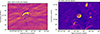 |
Fig. 2. Total intensity images of two magnetars with an SNR association. Left: SGR 1935+2154 at the S1-band, right: 1E1841-054 at L-band. |
The primary field of view of the telescope is much larger than that of the coherently formed beam. Hence, we are also able to see sources that are close to our original targets in our images. We make use of this to apply the imaging-based searches for radio emission to the (unconfirmed) magnetar candidate SGR 1808-20, which is in the images of the SGR 1806-20 observation and was dropped from our original target list due to the limited observation time.
In addition, the ultra-long period object ASKAP J1935+2148, close to SGR 1935+2154 and discovered by Caleb et al. (2024), which suggest it might be a slowly rotating magnetar, was captured during the imaging observations. The (potential) slowly rotating magnetar ASKAP J1935+2148 was not discovered at the time of writing the proposal, but the possibility of being the slowest rotating magnetar made it a target of interest in the search for radio emission. Moreover, during the creation of the images, we note that the sources SGR 1627-41 and CXOU J171405.7-381031 were observed with an offset larger than 1°. Hence, the data for this imaging epoch are not used (for both time and image domain).
3.2.2. Polarisation images
The two imaging epochs were also observed with a polarisation calibrator. Thus, we can create Stokes V images. This is useful as diffuse emission is often bright in Stokes I but (almost) invisible in Stokes V, while the few objects that are emitting circular polarisation, which includes magnetars and pulsars, will stand out from their environment. Thus, to create Stokes V images, we make use of the pipeline developed for the Max Planck Institute for Radio Astronomy MeerKAT Galactic Plane Survey (Padmanabh et al. 2023) (MMGPS)4, since oxkat does not yet support this step.
3.2.3. Imaging light curves
Single pulses can also be searched for in the image domain by creating a time series with the time resolution of the images being taken. Given that the images were taken in 8 s intervals, we can create a light curve of the position of the source. This approach is similar to the search for emission of ultra-long period transients. This also helps to protect against RFI signals that originate from Earth. For creating so-called snapshot images, we use fully calibrated total intensity images and create images without cleaning but subtracting the model (the mean value of each pixel) to focus on the transient emission only. Given the length of the observation, we get 112 images per source, which corresponds to 112 time bins. For each image, we average the area with a 5″ radius around the source position. This area is somewhat smaller than the typical beam for a point source as we focus on the bright centre of the source’s position. The results are the light curves for each magnetar, and ASKAP J1935+2148 displayed in Fig. 3 and Fig. C.1, which we visually inspect for any signal greater than three times the standard deviation after subtraction of the mean of the light curve.
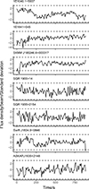 |
Fig. 3. Normalised (and model subtracted) light curves (solid lines) and +−3 sigma limits (dashed lines) for each source for the S1-band observation for the magnetars as well as ASKAP J1935+2148, which is in the beam of the SGR 1935+2154 observation. The time resolution is 8 s. |
4. Results
4.1. Beam forming
In the two beam-forming searches, no single pulse or folded profile that can be related to the magnetars has been found above the S/N threshold of 6. Nevertheless, our observations showed several notable re-detections of pulsars in the proximity of our targeted magnetars, both in single pulses and folding searches. The most notable is the detection of the pulsar B1641-45 in the beam of CXOU J164710.2-455216, which has been seen when folding with the period of the magnetar itself, but also many single pulses were discovered (Fig. A.1). Given the DM of 478 pc/cm3 and the periodicity of 455ms, these pulses can easily be related to PSR B1641-45. Its angular distance is 0.42° from CXOU J164710.2-455216. Additionally, it clearly demonstrates that our pipeline BLISS is able to blindly find single pulses of a source in the beam. However, this clearly limits the detectability of single pulses from the magnetar itself, as the pulsar period is about 4% of the magnetar. Additionally, since both sources are in the proximity of the Westerlund I cluster, their DM is potentially also quite similar. This makes distinguishing between a single pulse from the magnetar and the pulsar challenging.
We additionally found single pulses from a pulsar when inspecting the data from the magnetar SGR 1627-41. As these were three pulses separated by about 440 ms with a DM of 470 pc/cm3, they can be related to the pulsar PSR B1630-44, which happened to be in the beam due to the spurious 1° offset in this observation.
For our main sources, magnetars, we can thus only give upper limits for the radio fluence of single pulses and the mean radio flux density of the folded profiles. We estimate the upper limit mean flux density Smean and the upper limit single pulse fluence FSP using the respective version of the radio meter equation:
where (S/N) = 7 is the minimal S/N of the folded profile or the single pulse, respectively, Tsys is the system temperature, G is the gain, npol = 2 is the number of polarisations recorded, tobs is the duration of the observation, B is the bandwidth of the receiver, X is the duty cycle, Z is the correction factor for the red noise contribution, and w is the single pulse width. We adopt the same values as used in Younes et al. (2025) for the telescope-dependent properties. That is G = 2.65 K/Jy and Tsys = 26 K for the L-band observations and an SEFD = Tsys/G for 56 antennas of 8.6 Jy for the S1-band observations. To estimate Z, we compare the RMS of the residual FFT in the millisecond regime to the RMS in the regime of the period of the slowest magnetar (12 s). This gives a factor of about 4 and thus Z ≈ 4.
For the regular L-band and S1-band observations we estimate Smean = 68 μJy, FSP = 52mJyms and Smean = 52 μJy, FSP = 39mJyms respectively. The last two observations with commensal imaging (one in each band) were slightly longer, so the upper limits for Smean are 60 μJy (L-band) and 43.6 μJy (S1-band). Using the distance estimates of the magnetars, we can estimate the corresponding luminosity and single pulse energy as upper limits. These values are listed in Sect. 2.
Overview of the upper limits from both time and imaging domain.
4.2. Imaging
Figure 2 shows two examples of the resulting total intensity images: S1-band for SGR 1935+2154 and L-band for 1E1841-045. For each of the two sources, the associated SNR is clearly visible. For the SGR 1935+2154 images, we also marked the position of the ultra-long period transient discovered by Caleb et al. (2024). For both sources, the associated SNR is visible. Considering the magnetars as point sources, we searched for them as their respective positions by inspecting the Stokes I and Stokes V images. However, we did not find any radio point-source association for any of the magnetars considered. In the case of SGR 1806-20, we find some emission at the position of the source. After further inspection, it appears most likely to be diffuse emission of the surrounding ISM due to the non-point source like appearance of the emission. Moreover, there is no emission at this position in Stokes V. Hence, we derive upper limits from the imaging domain on the persistent radio emission of each magnetar. To do so, we estimate the RMS of the magnetar in a circle with a radius of 30″ around the magnetar’s position. To be detectable, we require that a source is at least seven times the RMS, which is a threshold inferred by other point sources in the images. The corresponding values for the total intensity images are listed in Sect. 2, where the luminosity using the distance is also estimated. For sources, which are located in an area of diffuse emission (such as SGR 1806-20), the upper limits are higher as a consequence. As the diffuse emission is (almost) completely gone in the Stokes V images, here the upper limit for non-detections is the same among the different sources and about 2 × 10⁻⁴ Jy/beam in the L-band and 2.1 × 10⁻⁴ Jy/beam for the S1-band observation, respectively.
For the light curves obtained from the images shown in Fig. C.1 and Fig. 3, we do not find any signal above our detection threshold in the imaging time series, despite an outlier for SGR 1935+2154. Inspecting the corresponding images and beam-forming candidates around the outlier reveals no signal of interest. Applying the somewhat more conservative threshold for a detection of seven times the RMS, we estimate an upper limit for each light curve for the flux density and luminosity, respectively. Both are listed in Sect. 2.
Despite the non-detection of radio emission from our main targets (the magnetars), we can clearly see that the environment of these sources is very complex, which explains the rather high DM estimates for most of the sources. We find several pulsars in the imaging domain, such as PSR J1841-0500 in the S1-band observation, which is an intermittent pulsar with a substantial amount of circular polarisation (Camilo et al. 2012). As some of the pulsars are visible in the circular polarisation images, we can confirm the quality of our images and that the non-detections of the magnetars in the Stokes V images are indeed astrophysical.
Additionally, the images give a view of the environment of the magnetars themselves and their associated structures, such as SNRs. All images of the sources are presented in Figure 2 and Figure B.1. Clearly, the SNRs of SGR 1935+2154 and 1E1841-045 can be identified in their images at both the L- and S-bands. Even the other magnetars are located in complex environments, which, given their location close to the galactic plane, is not surprising.
5. Discussion
The non-detection of any radio signal from the targeted magnetars can be because 1.) they are indeed radio quiet during our observations, or because 2.) there was emission that we could not detect. Reasons for the latter include a weak source that we were not sensitive to, an unfortunate beaming angle, effects of the interstellar medium, such as scattering or diffuse emission (for imaging only), which diminish the signal from the source, or a combination of all of them.
Although the general emission mechanism of magnetars is unclear, there are some arguments one can try to make to rule out radio emission from magnetars based on their physical properties. Szary et al. (2015) extend the partial screen gap model from radio pulsars into the magnetar regime, making the radio emission rotationally powered, and thus one can make predictions on whether a magnetar emits radio or not based on the temperature in its quiescent state and the period and period derivative. Based on the arguments made by Szary et al. (2015), the following magnetars should not emit radio emission: 1E 1048.1-5937, 1E 1841-045, 1RXS J170849.0, CXOU J164710.2, SGR 1806-20, SGR 1900+14, and Swift J1822.3-1606, either because of a too high surface temperature or too strong magnetic fields.
In addition to the traditional emission mechanism powered by rotational energy, emission mechanisms powered by strong magnetic fields have been proposed. Wang et al. (2019) argue that the emission of the radio loud magnetars XTE J1810-197 and PSR J1622-4950 is powered by oscillations in the magnetosphere, which are induced by a quake of the crust of the magnetar. Additionally, Wang et al. (2024) argue that the radio emission seen in SGR 1935+2154 during the detection of several weak radio pulses is powered by the untwisting magnetic field in the outer magnetosphere. Cooper & Wadiasingh (2024) extend this model to ultra-long period transients, arguing that they are magnetically powered, but also noting that the normal magnetars, that is, the magnetars considered in this work, are too young and might not have built up enough twist in the magnetosphere to sustain the magnetic radio emission. As the death lines and the fundamental plane of magnetars Rea et al. (2012b) are based on rotational powered radio emission, these cannot make predictions on the radio emission of magnetars that are powered on the magnetic field.
Although the process that initiated radio emission differs between rotationally powered and magnetically powered models, the opening angle of the open field line region (or its equivalent in the case of magnetically powered radio emission) defines the beaming fraction (as discussed by Beloborodov 2009), that is, the region of the sky illuminated by the beam. The beaming fraction is thus another limiting factor in the detectability of radio emission. While for ordinary radio pulsars this is commonly estimated from the open field line polar cap geometry and empirical fits (for example Tauris & Manchester 1998), magnetars generally do not follow the narrow polar cap picture. As shown by, for example, Philippov & Kramer (2022), the beam widths of magnetars are about an order of magnitude larger than those of radio pulsars, which indicates that their beaming fractions are also much larger (these would correspond to a beaming fraction of 4% if the pulsar-based polar cap model were applied to these periods). Thus, the non-detection of radio emission from all 13 magnetars is therefore unlikely to be due solely to geometrical effects.
Our understanding of magnetar radio emission is heavily biased due to the small sample of known radio loud magnetars. The strong increase in the flux density of XTE J1810-197 in mid-2020 and early 2021 without notable X-ray activity (Caleb et al. 2022; Bause et al. 2024) and the temporary radio quietness of 1E 1547.0-5408 after an X-ray outburst Lower et al. (2023) deviate from the commonly assumed X-ray radio relation. Additionally, some radio loud magnetars are emitting in radio only sporadically, like SGR 1935+2154. Thus, defining a ‘regular’ radio loud magnetar is challenging, as so far the class appears to consist of many special cases.
Additional challenges in detecting the radio emission from magnetars are their distances, making them faint, and their environment, which influences the emitted radio emission. The estimated DMs and τ for the magnetars are very high compared to the typical galactic radio pulsar, which is challenging in the search for radio emission in the time domain, especially at lower frequencies due to strongly scattered radio emission. This is due to their tendency to be in more complex structures, where a lot of material is in the lines of the side to us, as can be seen in the images in this work. τ is highly frequency dependent and thus changing to higher frequencies significantly reduces the effect of scattering. Although it is generally assumed that magnetars have flat spectra in contrast to radio pulsars, this finding originates from the small set of magnetars where enough radio emission has been observed. Hence, moving to higher frequencies to avoid scattering might still cause a reduced brightness if the spectrum is not flat or has a turn-over, as seen for XTE J1810-197 (Maan et al. 2022). In this particular case, the turn-over is thought to originate from free-free absorption, which limits the detectable radio flux. Given that a large number of magnetars are located in dense regions of the Milky Way and free-free absorption can occur, it could impact their detectability as well. The imaging domain, on the other hand, does not suffer from scattering and is still able to detect pulsed emission that has been scattered so strongly that the profile or single pulses are not detectable anymore in beam-formed searches.
Using radio loud magnetars, the ratio η between the X-ray flux (FX) and the radio flux from the mean flux density (FR) can be estimated. We selected the X-ray flux from a quiescent stage to avoid a potential influence on η from the outburst mechanism. For the radio loud magnetars, we tried to find fluxes close in time to 1E 1547.0-5408 (radio + X-ray: Lower et al. 2023), PSR J1622-4950 (radio: Scholz et al. 2017, X-ray: Coelho et al. 2017), SGR J1745-2900 (radio: Eatough et al. 2013, X-ray: Rajwade et al. 2022), Swift J1818.0-1607 (radio + X-ray : Rajwade et al. 2022), and XTE J1810-197 (radio: Bause et al. 2024). As the radio profile of SGR 1935+2154 was only visible for a very short period by FAST (Zhu et al. 2023), we used the simultaneous X-ray and radio observation of a burst with η ≈ 2.5 ⋅ 107 (Bochenek et al. 2020) instead, to give a reference noting that this is a different characteristic than for the other magnetars, and a galactic FRB would likely saturate the MeerKAT receivers. Figure 4 shows η for each of the five targets. Additionally, we estimated the flux limit, and thus the limit on η, using our radio upper limits, and display them in Figure 4. For the estimates, we take FX from Olausen & Kaspi (2014) and Coti Zelati et al. (2018).
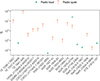 |
Fig. 4. X-ray to radio flux ratio for the radio loud and radio quiet magnetars. For SGR 1935+2154, both the radio quiet (from our measurements) as well as the radio loud one from the FRB-like burst are shown (star shape). |
Sources with η larger than the radio-loud ones should be detectable in our search. Clearly, all magnetars except Swift J1834.9-0846 lie above the η values for the radio loud magnetars. This suggests either that η is not a universal characteristic in the magnetar population or that these sources are not emitting radio in a manner consistent with the radio loud subclass during our observational window. Consequently, the lack of detection in our survey may reflect the aforementioned reasons: intrinsic differences in radio emission mechanisms, temporal variability, their dense environment, or viewing geometry. This might imply that the radio emission from most magnetars could be fundamentally distinct from that of their radio loud counterparts. Further radio monitoring of magnetars is required to constrain this.
The ongoing and upcoming all-sky surveys, such as the ASKAP Variables and Slow Transients survey (VAST; Murphy et al. (2013)), BURSTT (Lin et al. 2022), the SKA, CHORD (Vanderlinde et al. 2019), or DSA-2000 are ideal instruments that can deliver a very high cadence of observations of a large sky fraction that also includes positions of many radio quiet magnetars. We encourage these instruments to also monitor for any radio activity from magnetars using both the imaging and the time domain.
6. Conclusion
In this work, we present the results of an eight-month-long monitoring campaign of 12 radio quiet magnetars and SGR 1935+2154 using the MeerKAT interferometer radio telescope. While focused on the time domain, we also make use of MeerKAT’s interferometric nature and the powerful data taking back end for a search for radio emission in the image domain. Thus, we can search for radio emission from four different perspectives:
-
The FRB perspective by blindly searching for (faint) single pulses of widths from the time resolution to the period of the magnetar over a DM range from 20 pc/cm3 to 10 000 pc/cm3. The non-detections give upper limits of 52 mJyms (L-band) and 39 mJyms (S1-band) for a 10 ms burst.
-
The radio pulsar perspective by folding the observations to search for pulsed emission using both an FFT and an FFA approach. For L-band observations, we can report the upper limits of 68 μJy, while for the S1-band, we can report the upper limits of 56 μJy for each source during our observational campaign.
-
The persistent radio emission perspective by searching for point sources at the positions of the magnetars in the epochs, where the full calibrator scheme for the imaging domain was followed. Our upper limits depend on the environment of the source and are of the order of ≈0.5 mJy/beam for most sources.
-
The long duration single pulse or long duty cycle perspective, that is, searching for single pulses in the image domain by using 8 s snapshot images at the position of the magnetars and generating a light curve for each source. The upper limits are about ⪅0.1 mJy/beam.
In addition to the 13 magnetars specifically targeted, we make use of the field of view of MeerKAT in the imaging domain to also report upper limits for the ultra-long period transient ASKAP J1935+2148 and the magnetar SGR 1808-20 and re-detect several radio pulsars.
We find our results partially in agreement with the models trying to predict radio emission from magnetars, but argue that the foundation of magnetars used in magnetar emission models might not be sufficient because several magnetars are special cases. Hence, we highly encourage follow-up and reports of non-detection of radio quiet magnetars with high cadence, independent of X-ray activity of the magnetar. Ideally, searches will be done in as many of the four perspectives as possible to gain a broader view of the magnetar’s potential of emitting in the radio regime and thus help to understand their emission mechanism, as well as connected phenomena such as FRBs.
Data availability
The final images presented in this work are available in the CDS. The raw measurement sets taken from MeerKAT, as well as the raw time domain data, are available from the MeerKAT data archive. The intermediate filterbanks and light curves are stored at the archive of the Max-Planck-Institute for radio astronomy and can be shared upon reasonable request. The images of Figure B.1 and Figure B.2 are available at the CDS via https://cdsarc.cds.unistra.fr/viz-bin/cat/J/A+A/708/A321.
Acknowledgments
L.G.S. is a Lise Meitner Group Leader, and together with M.L.B. acknowledge support from the Max Planck Society. The MeerKAT telescope is operated by the South African Radio Astronomy Observatory, which is a facility of the National Research Foundation, an agency of the Department of Science and Innovation. This work has made use of the ‘MPIfR S-band receiver system’ designed, constructed, and maintained by funding of the MPI für Radioastronomy and the Max Planck Society. Observations used PTUSE for data acquisition, storage, and analysis which was partly funded by the Max-Planck-Institut für Radioastronomie (MPIfR). We acknowledge the MMGPS pipeline (https://www.mpifr-bonn.mpg.de/mmgps) development team for helping in part with the data analyses. We thank the anonymous referee for the fruitful comments.
References
- Aharonian, F., Akhperjanian, A. G., BarresdeAlmeida, U., et al. 2008, A&A, 486, 829 [NASA ADS] [CrossRef] [EDP Sciences] [Google Scholar]
- An, H., & Archibald, R. 2019, ApJ, 877, L10 [Google Scholar]
- Anderson, P. W., & Itoh, N. 1975, Nature, 256, 25 [NASA ADS] [CrossRef] [Google Scholar]
- Archibald, R. F., Scholz, P., Kaspi, V. M., Tendulkar, S. P., & Beardmore, A. P. 2020, ApJ, 889, 160 [Google Scholar]
- Bai, J., Wang, N., Dai, S., et al. 2025, ApJ, 979, 122 [Google Scholar]
- Barthelmy, S. D., Sakamoto, T., Baumgartner, W. H., et al. 2010, GRB Coordinates Network, 10528, 1 [Google Scholar]
- Bause, M. L., Herrmann, W., & Spitler, L. G. 2024, A&A, 686, A144 [NASA ADS] [CrossRef] [EDP Sciences] [Google Scholar]
- Beloborodov, A. M. 2009, ApJ, 703, 1044 [NASA ADS] [CrossRef] [Google Scholar]
- Bochenek, C. D., Ravi, V., Belov, K. V., et al. 2020, Nature, 587, 59 [NASA ADS] [CrossRef] [Google Scholar]
- Borghese, A., Rea, N., Turolla, R., et al. 2019, MNRAS, 484, 2931 [NASA ADS] [CrossRef] [Google Scholar]
- Burgay, M., Rea, N., Israel, G. L., et al. 2006, MNRAS, 372, 410 [Google Scholar]
- Caleb, M., Rajwade, K., Desvignes, G., et al. 2022, MNRAS, 510, 1996 [Google Scholar]
- Caleb, M., Lenc, E., Kaplan, D. L., et al. 2024, Nat. Astron., 8, 1159 [NASA ADS] [CrossRef] [Google Scholar]
- Camilo, F., & Reynolds, J. 2007, ATel, 1056, 1 [Google Scholar]
- Camilo, F., Ransom, S. M., Halpern, J. P., & Reynolds, J. 2007, ApJ, 666, L93 [NASA ADS] [CrossRef] [Google Scholar]
- Camilo, F., Ransom, S. M., Chatterjee, S., Johnston, S., & Demorest, P. 2012, ApJ, 746, 63 [Google Scholar]
- Camilo, F., Ransom, S. M., Halpern, J. P., et al. 2016, ApJ, 820, 110 [NASA ADS] [CrossRef] [Google Scholar]
- Chen, K., & Ruderman, M. 1993, ApJ, 402, 264 [NASA ADS] [CrossRef] [Google Scholar]
- CHIME/FRB Collaboration (Andersen, B. C., et al.) 2020, Nature, 587, 54 [Google Scholar]
- Coelho, J. G., Cáceres, D. L., de Lima, R. C. R., et al. 2017, A&A, 599, A87 [NASA ADS] [CrossRef] [EDP Sciences] [Google Scholar]
- Cooper, A. J., & Wadiasingh, Z. 2024, MNRAS, 533, 2133 [Google Scholar]
- Coti Zelati, F., Rea, N., Pons, J. A., Campana, S., & Esposito, P. 2018, MNRAS, 474, 961 [NASA ADS] [CrossRef] [Google Scholar]
- Crawford, F., Hessels, J. W. T., & Kaspi, V. M. 2007, ApJ, 662, 1183 [Google Scholar]
- Cummings, J. R., Burrows, D., Campana, S., et al. 2011, ATel, 3488, 1 [NASA ADS] [Google Scholar]
- D’Elia, V., Barthelmy, S. D., Baumgartner, W. H., et al. 2011, GRB Coordinates Network, 12253, 1 [Google Scholar]
- Dib, R., & Kaspi, V. M. 2014, ApJ, 784, 37 [NASA ADS] [CrossRef] [Google Scholar]
- Duncan, R. C., & Thompson, C. 1992, ApJ, 392, L9 [Google Scholar]
- Durant, M., & van Kerkwijk, M. H. 2006, ApJ, 648, 534 [Google Scholar]
- Eatough, R., Karuppusamy, R., Kramer, M., et al. 2013, ATel, 5040, 1 [Google Scholar]
- Esposito, P., Tiengo, A., Mereghetti, S., et al. 2009, ApJ, 690, L105 [Google Scholar]
- Esposito, P., Israel, G. L., Turolla, R., et al. 2011, MNRAS, 416, 205 [Google Scholar]
- Gaensler, B. M. 2014, GRB Coordinates Network, 16533, 1 [NASA ADS] [Google Scholar]
- Gaensler, B. M., Kouveliotou, C., Gelfand, J. D., et al. 2005a, Nature, 434, 1104 [NASA ADS] [CrossRef] [PubMed] [Google Scholar]
- Gaensler, B. M., McClure-Griffiths, N. M., Oey, M. S., et al. 2005b, ApJ, 620, L95 [NASA ADS] [CrossRef] [Google Scholar]
- Gavriil, F. P., Kaspi, V. M., & Woods, P. M. 2002, Nature, 419, 142 [CrossRef] [Google Scholar]
- Gelbord, J. M., & Vetere, L. 2010, GRB Coordinates Network, 10531, 1 [Google Scholar]
- Gogus, E., & Kouveliotou, C. 2011, ATel, 3542, 1 [Google Scholar]
- GöǧüŞ, E., Woods, P. M., Kouveliotou, C., et al. 1999, ApJ, 526, L93 [CrossRef] [Google Scholar]
- Gogus, E., Strohmayer, T., Kouveliotou, C., & Woods, P. 2010, GRB Coordinates Network, 10534, 1 [Google Scholar]
- Gogus, E., Kouveliotou, C., Kargaltsev, O., & Pavlov, G. 2011, ATel, 3576, 1 [NASA ADS] [Google Scholar]
- Guiriec, S., Kouveliotou, C., & van der Horst, A. J. 2011, GRB Coordinates Network, 12255, 1 [Google Scholar]
- Halpern, J. P., & Gotthelf, E. V. 2010a, ApJ, 725, 1384 [Google Scholar]
- Halpern, J. P., & Gotthelf, E. V. 2010b, ApJ, 710, 941 [Google Scholar]
- Halpern, J. P., Gotthelf, E. V., Becker, R. H., Helfand, D. J., & White, R. L. 2005, ApJ, 632, L29 [NASA ADS] [CrossRef] [Google Scholar]
- Heywood, I. 2020, oxkat: Semi-automated imaging of MeerKATobservations, Astrophysics Source Code Library [record ascl:2009.003] [Google Scholar]
- Hurley, K., Cline, T., Mazets, E., et al. 1999a, Nature, 397, 41 [NASA ADS] [CrossRef] [Google Scholar]
- Hurley, K., Li, P., Kouveliotou, C., et al. 1999b, ApJ, 510, L111 [NASA ADS] [CrossRef] [Google Scholar]
- Hurley, K., Boggs, S. E., Smith, D. M., et al. 2005, Nature, 434, 1098 [NASA ADS] [CrossRef] [Google Scholar]
- Karuppusamy, R., Desvignes, G., Kramer, M., et al. 2020, ATel, 13553, 1 [Google Scholar]
- Kaspi, V. M., & Beloborodov, A. M. 2017, ARA&A, 55, 261 [Google Scholar]
- Kirsten, F., Snelders, M. P., Jenkins, M., et al. 2021, Nat. Astron., 5, 414 [Google Scholar]
- Kouveliotou, C., Strohmayer, T., Hurley, K., et al. 1999, ApJ, 510, L115 [NASA ADS] [CrossRef] [Google Scholar]
- Kozlova, A. V., Israel, G. L., Svinkin, D. S., et al. 2016, MNRAS, 460, 2008 [NASA ADS] [CrossRef] [Google Scholar]
- Laros, J. G., Fenimore, E. E., Klebesadel, R. W., et al. 1987, ApJ, 320, L111 [Google Scholar]
- Lazarus, P., Kaspi, V. M., Champion, D. J., Hessels, J. W. T., & Dib, R. 2012, ApJ, 744, 97 [NASA ADS] [CrossRef] [Google Scholar]
- Levin, L., Bailes, M., Bates, S., et al. 2010, ApJ, 721, L33 [Google Scholar]
- Levin, L., Lyne, A. G., Desvignes, G., et al. 2019, MNRAS, 488, 5251 [Google Scholar]
- Lien, A. Y., Barthelmy, S. D., Baumgartner, W. H., et al. 2014, GRB Coordinates Network, 16522, 1 [NASA ADS] [Google Scholar]
- Lin, H.-H., Lin, K.-Y., Li, C.-T., et al. 2022, PASP, 134, 094106 [NASA ADS] [CrossRef] [Google Scholar]
- Lorimer, D. R., & Xilouris, K. M. 2000, ApJ, 545, 385 [NASA ADS] [CrossRef] [Google Scholar]
- Lower, M. E., Younes, G., Scholz, P., et al. 2023, ApJ, 945, 153 [Google Scholar]
- Lu, W.-J., Zhou, P., Wang, P., et al. 2024, ApJ, 963, 151 [Google Scholar]
- Maan, Y., Surnis, M. P., Chandra Joshi, B., & Bagchi, M. 2022, ApJ, 931, 67 [NASA ADS] [CrossRef] [Google Scholar]
- Mazets, E. P., Golenetskij, S. V., & Guryan, Y. A. 1979, Sov. Astron. Lett., 5, 343 [NASA ADS] [Google Scholar]
- Mazets, E. P., Golenetskii, S. V., Ilinskii, V. N., et al. 1981, Ap&SS, 80, 3 [NASA ADS] [CrossRef] [Google Scholar]
- Men, Y., & Barr, E. 2024, A&A, 683, A183 [NASA ADS] [CrossRef] [EDP Sciences] [Google Scholar]
- Men, Y., Barr, E., Clark, C. J., Carli, E., & Desvignes, G. 2023, A&A, 679, A20 [NASA ADS] [CrossRef] [EDP Sciences] [Google Scholar]
- Morello, V., Barr, E. D., Stappers, B. W., Keane, E. F., & Lyne, A. G. 2020, MNRAS, 497, 4654 [NASA ADS] [CrossRef] [Google Scholar]
- Muno, M. P., Clark, J. S., Crowther, P. A., et al. 2006, ApJ, 636, L41 [NASA ADS] [CrossRef] [Google Scholar]
- Murphy, T., Chatterjee, S., Kaplan, D. L., et al. 2013, PASA, 30 [Google Scholar]
- Olausen, S. A., & Kaspi, V. M. 2014, ApJS, 212, 6 [Google Scholar]
- Padmanabh, P. V., Barr, E. D., Sridhar, S. S., et al. 2023, MNRAS, 524, 1291 [NASA ADS] [CrossRef] [Google Scholar]
- Philippov, A., & Kramer, M. 2022, ARA&A, 60, 495 [NASA ADS] [CrossRef] [Google Scholar]
- Rajwade, K. M., Stappers, B. W., Lyne, A. G., et al. 2022, MNRAS, 512, 1687 [NASA ADS] [CrossRef] [Google Scholar]
- Ransom, S. M. 2001, Ph.D. Thesis, Harvard University, Massachusetts [Google Scholar]
- Rea, N., Israel, G. L., Esposito, P., et al. 2012a, ApJ, 754, 27 [NASA ADS] [CrossRef] [Google Scholar]
- Rea, N., Pons, J. A., Torres, D. F., & Turolla, R. 2012b, ApJ, 748, L12 [CrossRef] [Google Scholar]
- Rea, N., Viganò, D., Israel, G. L., Pons, J. A., & Torres, D. F. 2014, ApJ, 781, L17 [NASA ADS] [CrossRef] [Google Scholar]
- Scholz, P., Archibald, R. F., Kaspi, V. M., et al. 2014, ApJ, 783, 99 [NASA ADS] [CrossRef] [Google Scholar]
- Scholz, P., Camilo, F., Sarkissian, J., et al. 2017, ApJ, 841, 126 [Google Scholar]
- Seward, F. D., Charles, P. A., & Smale, A. P. 1986, ApJ, 305, 814 [Google Scholar]
- Shannon, R. M., & Johnston, S. 2013, MNRAS, 435, L29 [Google Scholar]
- Spitler, L. G., Cordes, J. M., Chatterjee, S., & Stone, J. 2012, ApJ, 748, 73 [CrossRef] [Google Scholar]
- Stamatikos, M., Malesani, D., Page, K. L., & Sakamoto, T. 2014, GRB Coordinates Network, 16520, 1 [NASA ADS] [Google Scholar]
- Sugizaki, M., Nagase, F., Torii, K., et al. 1997, PASJ, 49, L25 [Google Scholar]
- Szary, A., Melikidze, G. I., & Gil, J. 2015, ApJ, 800, 76 [Google Scholar]
- Tauris, T. M., & Manchester, R. N. 1998, MNRAS, 298, 625 [NASA ADS] [CrossRef] [Google Scholar]
- Testa, V., Mignani, R. P., Hummel, W., Rea, N., & Israel, G. L. 2018, MNRAS, 473, 3180 [Google Scholar]
- Thompson, C., & Duncan, R. C. 1993, ApJ, 408, 194 [NASA ADS] [CrossRef] [Google Scholar]
- Vanderlinde, K., Liu, A., Gaensler, B., et al. 2019, in Canadian Long Range Plan for Astronomy and Astrophysics White Papers, 2020, 28 [Google Scholar]
- Vasisht, G., & Gotthelf, E. V. 1997, ApJ, 486, L129 [Google Scholar]
- Vasisht, G., Kulkarni, S. R., Frail, D. A., & Greiner, J. 1994, ApJ, 431, L35 [Google Scholar]
- Voges, W., Aschenbach, B., Boller, T., et al. 1999, A&A, 349, 389 [NASA ADS] [Google Scholar]
- Wachter, S., Patel, S. K., Kouveliotou, C., et al. 2004, ApJ, 615, 887 [Google Scholar]
- Wang, Z., & Chakrabarty, D. 2002, ApJ, 579, L33 [Google Scholar]
- Wang, Z., Kaspi, V. M., & Higdon, S. J. U. 2007, ApJ, 665, 1292 [Google Scholar]
- Wang, W., Zhang, B., Chen, X., & Xu, R. 2019, ApJ, 875, 84 [Google Scholar]
- Wang, P., Li, J., Ji, L., et al. 2024, ApJS, 275, 39 [Google Scholar]
- Woods, P. M., Kouveliotou, C., van Paradijs, J., et al. 1999, ApJ, 519, L139 [Google Scholar]
- Woods, P. M., Kaspi, V. M., Gavriil, F. P., & Airhart, C. 2011, ApJ, 726, 37 [Google Scholar]
- Xie, L., Han, J. L., Yang, Z. L., et al. 2025, Res. Astron. Astrophys., 25, 014004 [Google Scholar]
- Younes, G., Kouveliotou, C., Kargaltsev, O., et al. 2012, ApJ, 757, 39 [Google Scholar]
- Younes, G., Baring, M. G., Kouveliotou, C., et al. 2017, ApJ, 851, 17 [Google Scholar]
- Younes, G., Baring, M. G., Kouveliotou, C., et al. 2020, ApJ, 889, L27 [NASA ADS] [CrossRef] [Google Scholar]
- Younes, G., Baring, M. G., Harding, A. K., et al. 2023, Nat. Astron., 7, 339 [Google Scholar]
- Younes, G., Lander, S. K., Baring, M. G., et al. 2025, arXiv e-prints [arXiv:2502.20079] [Google Scholar]
- Zhou, P., Chen, Y., Li, X.-D., et al. 2014, ApJ, 781, L16 [CrossRef] [Google Scholar]
- Zhu, W., Xu, H., Zhou, D., et al. 2023, Sci. Adv., 9 [Google Scholar]
Appendix A: Detection of the pulsar B1641-45 in the single pulse pipeline
Figure A.1 shows the detection of the pulsar B1641-45 in the BLISS pipeline.
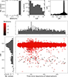 |
Fig. A.1. Overview of the single pulse detections of the pulsar in the Beam of CXOU1647 in an L-band observation. The top row of panels shows (from left to right) a histogram of the detected single pulse widths and S/N respectively as well as S/N vs. DM. The bottom part shows a DM vs. time scatter plot of all candidates, where each axis as a histogram added and the S/N of the candidates are given by the circle size while the width is given by the colour of the circles. |
Appendix B: MeerKAT images and light curves of all sources
In addition to the images presented in Fig. 2, Fig. B.1 and Fig. B.2 present the final, primary beam corrected images of the magnetars with the positions of the magnetars highlighted.
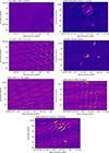 |
Fig. B.1. Further images of all other sources at L and S1-band. |
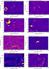 |
Fig. B.2. Images of all other sources at L-band |
Appendix C: MeerKAT light curves of all sources at L-band
Figure C.1 presents the light curves of each magnetar and the ultra-long period transient in the image of SGR 1935+2148 observed in the L-band imaging epoch.
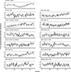 |
Fig. C.1. Normalised light curves (solid lines) and +-3 sigma limits (dashed lines) for each source for the L-band observation for the magnetars as well as the ULP ASKAP J1935+2148, which is in the beam of the SGR 1935+2154 observation. The time resolution is 8 s. |
All Tables
All Figures
|
Fig. 1. So-called P-Pdot diagram, which shows spin period (P) vs spin period derivative (Ṗ) for the radio loud (triangles) and the radio quiet magnetars considered in this work (circles). The values are taken from from Olausen & Kaspi (2014). Additionally, two death lines are shown: simple dipolar field magnetic field (upper line) and a twisted magnetosphere (bottom line). The area in between is referred to as the death valley. |
| In the text | |
|
Fig. 2. Total intensity images of two magnetars with an SNR association. Left: SGR 1935+2154 at the S1-band, right: 1E1841-054 at L-band. |
| In the text | |
|
Fig. 3. Normalised (and model subtracted) light curves (solid lines) and +−3 sigma limits (dashed lines) for each source for the S1-band observation for the magnetars as well as ASKAP J1935+2148, which is in the beam of the SGR 1935+2154 observation. The time resolution is 8 s. |
| In the text | |
|
Fig. 4. X-ray to radio flux ratio for the radio loud and radio quiet magnetars. For SGR 1935+2154, both the radio quiet (from our measurements) as well as the radio loud one from the FRB-like burst are shown (star shape). |
| In the text | |
|
Fig. A.1. Overview of the single pulse detections of the pulsar in the Beam of CXOU1647 in an L-band observation. The top row of panels shows (from left to right) a histogram of the detected single pulse widths and S/N respectively as well as S/N vs. DM. The bottom part shows a DM vs. time scatter plot of all candidates, where each axis as a histogram added and the S/N of the candidates are given by the circle size while the width is given by the colour of the circles. |
| In the text | |
|
Fig. B.1. Further images of all other sources at L and S1-band. |
| In the text | |
|
Fig. B.2. Images of all other sources at L-band |
| In the text | |
|
Fig. C.1. Normalised light curves (solid lines) and +-3 sigma limits (dashed lines) for each source for the L-band observation for the magnetars as well as the ULP ASKAP J1935+2148, which is in the beam of the SGR 1935+2154 observation. The time resolution is 8 s. |
| In the text | |
Current usage metrics show cumulative count of Article Views (full-text article views including HTML views, PDF and ePub downloads, according to the available data) and Abstracts Views on Vision4Press platform.
Data correspond to usage on the plateform after 2015. The current usage metrics is available 48-96 hours after online publication and is updated daily on week days.
Initial download of the metrics may take a while.