| Issue |
A&A
Volume 709, May 2026
|
|
|---|---|---|
| Article Number | A93 | |
| Number of page(s) | 9 | |
| Section | Interstellar and circumstellar matter | |
| DOI | https://doi.org/10.1051/0004-6361/202659347 | |
| Published online | 05 May 2026 | |
Tentative detection of the glycine isomer glycolamide in a hot molecular core
1
School of Chemistry and Chemical Engineering, Chongqing University,
Daxuecheng South Rd. 55,
Chongqing
401331,
PR China
2
Chongqing Key Laboratory of Chemical Theory and Mechanism, Chongqing University,
Daxuecheng South Rd. 55,
Chongqing
401331,
PR China
3
Max Planck Institute for Astronomy,
Königstuhl 17,
Heidelberg
69117,
Germany
4
Department of Physics, Xi’an Jiaotong-Liverpool University,
Ren’ai Road 111,
Suzhou
215123,
PR China
5
LUX, Observatoire de Paris, PSL Research University, CNRS, Sorbonne Universités,
Paris
75014,
France
6
Center for Astrophysics, GuangZhou University,
Guangzhou
510006,
PR China
★ Corresponding authors: This email address is being protected from spambots. You need JavaScript enabled to view it.
; This email address is being protected from spambots. You need JavaScript enabled to view it.
Received:
6
February
2026
Accepted:
5
April
2026
Abstract
Understanding whether prebiotic molecules can endure and reform through the energetic stages of star formation is essential for tracing the continuity of interstellar chemistry toward life. Glycolamide, an isomer of glycine, was recently detected in the molecular cloud G+0.693-0.027. However, establishing its presence in warm, high-density environments is crucial to evaluate the chemical continuity of amides. Here we report the tentative detection of glycolamide in a hot molecular core, G358.93-0.03 MM1, using ALMA 1 mm observations. Seven unblended or only mildly blended emission lines were identified, yielding an abundance of (1.7±0.2)×10−10 relative to H2. The comparable formamide/glycolamide and acetamide/glycolamide abundance ratios in both sources suggest a chemically connected amide network across different environments. These results demonstrate that amides can persist and chemically evolve during massive star formation, tracing the chemical continuity from interstellar to protostellar environments.
Key words: astrochemistry / ISM: abundances / ISM: molecules
© The Authors 2026
 Open Access article, published by EDP Sciences, under the terms of the Creative Commons Attribution License (https://creativecommons.org/licenses/by/4.0), which permits unrestricted use, distribution, and reproduction in any medium, provided the original work is properly cited.
This article is published in open access under the Subscribe to Open model. This email address is being protected from spambots. You need JavaScript enabled to view it. to support open access publication.
1 Introduction
The emergence of life on Earth dates back to ∼3.8 billion years ago (Pearce et al. 2018), yet the astrochemical origin of its fundamental molecular building blocks remains unclear. Among the wide variety of prebiotic molecules, amino acids are of particular interest because they constitute the monomeric units of proteins, which play pivotal catalytic and metabolic roles in living systems (Pizzarello & Weber 2004; Weber & Pizzarello 2006; Wu 2009). Their identification in meteorites (Cronin & Pizzarello 1983; Burton et al. 2012) and samples returned from asteroid Ryugu (Potiszil et al. 2023) and comet 67P/Churyumov-Gerasimenko (Altwegg et al. 2016) implies that part of amino acid chemistry may trace back to interstellar or protosolar stages, motivating systematic searches for these species in the interstellar medium.
Glycine (NH2CH2COOH), the simplest amino acid, has long been the prime target for astronomical searches because it is thought to be among the easiest bio-monomers to assemble under interstellar conditions (Ruiz-Mirazo et al. 2014). Despite this expectation, all previous attempts have failed to yield a secure detection. Early claims toward several high-mass star-forming regions were latter refuted (Kuan et al. 2003; Snyder et al. 2005). Subsequent, more sensitive observations toward the high-mass star-forming region SgrB2 (Combes et al. 1996; Jones et al. 2007; Cunningham et al. 2007), Orion KL (Combes et al. 1996; Cunningham et al. 2007), the molecular cloud G+0.693-0.027 (Jiménez-Serra et al. 2020), the low-mass protostar IRAS 16293-2422 (Jiménez-Serra et al. 2020; Ceccarelli et al. 2000), and the pre-stellar core L1544 (Jiménez-Serra et al. 2016) have not confirmed its presence either. This persistent non-detection has reshaped the field’s approach – from direct glycine searches toward indirect chemical diagnostics, with a focus on its structural isomers and related species that may be more abundant or more readily observable.
Glycine belongs to the C2H5O2N family, several members of which have been characterized spectroscopically, including methyl carbamate (CH3OC(O)NH2; Marstokk & Mollendal 1999; Bakri et al. 2002; Ilyushin et al. 2006), the syn- and anti-isomers of glycolamide (HOCH2C(O)NH2; Maris 2004; Sanz-Novo et al. 2020), and the Z- and E-isomers of acetohydroxamic acid (CH3C(O)NHOH; Sanz-Novo et al. 2022). These spectroscopic studies have enabled dedicated astronomical searches for C2H5O2N isomers toward a variety of interstellar sources, but most of them remain undetected (Demyk et al. 2004; Sanz-Novo et al. 2020; Colzi et al. 2021; Sanz-Novo et al. 2022). In this context, glycolamide in its syn-form (syn-HOCH2C(O)NH2, hereafter GA) is of particular interest because its hydroxyl and amide groups can form an intramolecular hydrogen bond, which stabilizes the structure and enhances its dipole moment, favoring its detection at millimeter wavelengths. GA was recently identified toward the G+0.693-0.027 molecular cloud with an abundance of ∼5.5×10⁻¹¹ relative to H2 (Rivilla et al. 2023). This detection provided the first observational evidence that a glycine structural isomer – a direct molecular analog of an amino acid – can form and persist under low-UV interstellar conditions.
Recent studies have suggested that GA may be of potential prebiotic interest, for instance as a precursor to key prebiotic molecules: the carbon–oxygen bond cleavage yields acetamide (CH3C(O)NH2) and ethanolamine (HOCH2CH2NH2) – a crucial molecular building block that serves as the head group in phosphatidylethanolamine, a constituent of both eukaryotic and bacterial membranes (Bergantini et al. 2025). Furthermore, GA can participate in polycondensation reactions to form N-(2-amino-2-oxoethyl)-2-hydroxyacetamide, a derivative of the glycine dipeptide. This raises the possibility that GA provides an alternative pathway for peptide formation in interstellar environments (Szőri et al. 2011; Rivilla et al. 2023; Perrero et al. 2025).
Testing whether amides like GA endure as interstellar ices and then warm and reprocess in protostellar cores is essential, because star formation subjects molecules to intense heating and radiation (Millar 2020). If such amino-acid-related species can persist or reform under these conditions, it would demonstrate that amide chemistry is robust enough to survive the transition from interstellar clouds to nascent stellar systems. Hot molecular cores (HMCs) – compact (≤0.1 pc), dense (n≥106 cm−3), and warm (T≥100 K) regions associated with massive protostars during the deeply embedded stage of star formation – provide ideal natural laboratories for such tests. During this stage, ice mantle sublimation, radical-radical reactions during warm-up, and subsequent gas-phase processing jointly drive the emergence of molecular complexity (Shimonishi et al. 2021; Duan et al. 2025a).
To explore whether amino-acid-related chemistry extends into these protostellar environments, we investigated the presence of GA in the HMC G358.93-0.03 MM1 (hereafter G358.93 MM1) – the brightest of eight submillimeter sources in the high-mass star-forming G358.93-0.03 complex (MM1-MM8; Brogan et al. 2019). G358.93 MM1 exhibits exceptionally line-rich spectra and a chemically diverse inventory, including prebiotic and amide-related molecules such as acetonitrile CH3CN, cyanamide NH2CN, glycolaldehyde CH2OHCHO, methylamine CH3NH2, ethylene glycol (CH2OH)2, isocyanic acid HNCO, and formamide NH2CHO (Manna & Pal 2023; Manna et al. 2023; Manna & Pal 2024; Manna et al. 2024). This chemical richness makes G358.93 MM1 an ideal testbed to investigate GA and its potential linkage to other amides.
Using ALMA 1 mm observations, we report the tentative detection of GA in an HMC. We derived its abundance relative to H2 and to related formamide and acetamide to probe possible chemical connections and formation pathways. The structure of this paper is as follows: Section 2 outlines the observations and data reduction, Sect. 3 presents the spectral analysis, Sect. 4 discusses the chemical implication, and Sect. 5 summarizes the conclusions.
2 Observation and data reduction
2.1 Observation
The high-mass star formation region G358.93-0.03 was observed using the Atacama Large Millimeter/Submillimeter Array (ALMA) band-7 receivers (Project ID: 2019.1.00768.S; PI: Crystal Brogan). The observation of G358.93-0.03 was carried out on 2021 May 17, with a phase center of RA(J2000) = 17h43m10s.000, Dec(J2000) = −29◦51′46.″000 and a total on-source integration time of 2963.52 s. A total of 47 antennas were used in the array, providing baseline lengths from 14 m to 2517 m. J1550+0527, a standard quasar used for calibration, served as both the flux and bandpass calibrator to determine the absolute flux scale and instrumental response. J1744-3116, located near the target field, was adopted as the phase calibrator to correct for short-term atmospheric and instrumental phase variations. The ALMA correlator was configured in dual-polarization mode, covering four spectral windows centered at 290.5–292.4, 292.5–294.3, 302.5–304.4, and 304.2–306.1 GHz. Each spectral window provided a resolution of 488.24 kHz, corresponding to a velocity resolution (δV) of ∼0.5 km s−1.
2.2 Data reduction
Calibration of the visibility data and subsequent imaging were carried out using the Common Astronomy Software Application (CASA; version 6.1.1.15; McMullin et al. 2007). The standard ALMA pipeline was first applied for initial calibration, including corrections for bandpass, flux, and phase variations.
Because G358.93 MM1 is a line-rich source, we first imaged the four spectral windows without continuum subtraction. We then used the line-free channels obtained by the CASA pipeline task findcont as an initial estimate for the continuum-fitting and iteratively excluded channels affected by line emission until no line-emission channels were found over 3σ. The remaining line-free channels were subsequently used for continuum fitting, while the line-emission channels were excluded from the continuum image construction. Three iterations of phase self-calibration were performed to improve phase stability, using solution intervals of “inf”, “30.25s”, and “int”, respectively. Each iteration employed a multi-term multifrequency synthesize deconvolver with two Taylor terms and multi-scale cleaning scales of 0, 5, 15, 50, and 150 pixels. Briggs weighting with a robust parameter of 0.5 was adopted throughout. After self-calibration, the continuum image quality improved substantially, yielding a synthetic beam of 0.15″×0.1″ (position angle –87.1◦) and an rms noise level of ∼20 uJy beam−1.
The final self-calibration solutions were applied to the original spectral-line data to correct phase errors across all channels. The continuum emission was then removed in the UV domain using the CASA task uvcontsub; the line-free channels were fitted with a first-order polynomial. Continuum-subtracted visibilities were imaged with the multi-scale deconvolver, using the same weighting scheme and scales (0, 5, 15, and 50 pixels). The Briggs weighting was used with a robust parameter of 0.5. The beam of each channel was restored into the common one for further wide-spectra analyses. The final line-cube sensitivity achieved was ∼0.5 K per 0.5 km s−1 channel, consistent with the expected thermal noise after self-calibration.
3 Results
3.1 Spectroscopic inputs and local thermodynamic equilibrium modeling
In this work we focused on GA together with the chemically related amides formamide (NH2CHO, hereafter FA) and acetamide (CH3C(O)NH2, hereafter AA). Spectroscopic data for these species were obtained from the Cologne Database for Molecular Spectroscopy (CDMS1; Müller et al. 2001, 2005). Table A.1 summarizes the corresponding database entries and literature sources used for the line parameters.
The observed spectra were modeled under the local thermodynamical equilibrium (LTE) assumption using CLASS/Weeds (Maret et al. 2011) sets of Grenoble Image and Line Data Analysis Software (GILDAS2). Five standard parameters were adopted in the model: source size (θ), line width (∆V), source velocity (VLSR), excitation temperature (Tex), and column density (Nt). To reduce parameter degeneracy, only Tex and Nt were treated as free parameters, and the other quantities were fixed as follows: θ was set to the deconvolved continuum sizes, ∆V to the average of Gaussian fits for bright unblended lines, and VLSR to - 16.5 km s−1 for G358.93 MM1 (Brogan et al. 2019). To refine the LTE parameters, we optimized the initial CLASS/Weeds model in CLASS/ADJUST using the Powell algorithm (Powell 1964) implemented in the SciPy optimization library. Because the uncertainties are dominated not only by the fitting procedure but also by line blending, baseline effects, and the simplifying assumptions of the LTE model, we adopted a conservative uncertainty of 20% for the derived Tex and Nt values.
Although line intensities peak near the continuum maximum, a detailed line-by-line inspection revealed that most GA transitions in this region suffer from significant blending with neighboring species, making reliable identification and fitting particularly challenging. This severe blending is primarily due to the strongest Doppler broadening toward the center, where lines are most significantly widened and overlapping. To mitigate this issue, spectra were extracted from slightly offset positions (Fig. 1b), where most of the GA lines are less affected by blending and display clean Gaussian profiles with high signal-to-noise ratios.
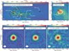 |
Fig. 1 (a) 1 mm continuum image of G358.93-0.03. Contour levels correspond to (20, 40, 80, 120, 200, 500, 1000, 1700) × σ, where σ is the rms noise level. The white ellipse in the lower-left corner indicates the synthesized beam of 0.15″×0.1″ (position angle –87.1◦). (b) Enlarged view of G358.93 MM1. The continuum peak is marked by a white cross, and the offset extraction position used for spectral analysis is marked by a red cross. (c–e) Integrated intensity (moment-0) maps of NH2CHO, CH3C(O)NH2, and syn-HOCH2C(O)NH2 toward G358.93 MM1, overlaid with the 1 mm continuum emission contours from panel (a). The color scale unit is Jy beam−1 km s−1. |
3.2 Molecular line identifications
Given the line-rich spectrum of G358.93 MM1, we constructed a full source model (Appendix B), including the molecules reported in previous studies and the species identified in this work, in order to assess potential blends and overlaps in the candidate GA lines. The spectroscopic entries used in this model were retrieved from three main databases: CDMS (Müller et al. 2001, 2005), the Jet Propulsion Laboratory (JPL) database3 (Pickett et al. 1998), and the Lille Spectroscopic Database (LSD4; Motiyenko & Margulès 2025). A complete list of all detected species is provided in Table B.1, together with the LTE parameters adopted for the full source model, including the excitation temperature (Tex), column density (Nt), line width (full width at half maximum), and velocity offset (Voff). For species other than GA, AA, and FA, these parameters were adjusted manually to best reproduce the observed spectrum. This full source model provides the basis for assessing possible blending and contamination in the candidate GA features.
Within this framework, GA is identified toward G358.93 MM1 through seven clean spectral features (Fig. 2), six of which are detected above the 3σ level and three above the 5σ level. Some of these clean features consist of multiple overlapping GA transitions at high K. Taken together, the clean features comprise 17 transitions associated with 7 distinct J values (see Table A.2) with upper-level energies (Eu) ranging from 108 to 389 K. All of these clean transitions are R-branch lines, including 7 a-type and 10 b-type transitions. Their relative intensities are well reproduced by the LTE model, and no stronger clean GA lines expected within the covered bands are missing from the observed spectrum. However, given the limited bandwidth (∼8 GHz), the modest number of securely detected transitions, and the high line density of this warm HMC, a coincidental assignment cannot be excluded with the confidence required for a firm detection claim. We therefore regard the identification as tentative. Under the LTE assumption, the best-fit model yields a column density of Nt(GA) = (5.3±1.1)×1014cm−2 and an excitation temperature of Tex(GA) = 102±20 K, with the linewidth of GA set to 1.4 km s−1.
As an independent consistency check on the best-fit LTE solution, we performed a rotational-diagram analysis based on seven unblended transitions of GA (Appendix C). The derived rotational temperature, Trot = 107±21 K, is in good agreement with the excitation temperature obtained from the best fit, supporting the reliability of the adopted LTE treatment.
We also assessed the robustness of the continuum subtraction by comparing our CASA-based procedure with STAT-CONT (Sánchez-Monge et al. 2018), an automated tool designed to determine the continuum level in line-rich spectra without manual intervention. The spectra produced by the two methods are nearly identical. The derived LTE parameters from the STATCONT-based spectra are also consistent with those from the CASA-based approach, although the column density derived from the STATCONT-based analysis is approximately 30% lower than that from the CASA-based approach (see Appendix D for details). This comparison indicates that the tentative GA identification is not driven by the particular continuum-subtraction method adopted.
Chemically related amides, FA and AA, were also examined. For FA, three unblended emission lines of the parent isotopolog and five of its 13C isotopolog ( ) were detected (see Fig. 3 and Table A.2). In the analysis, the line widths were fixed to the average values of 2.8 km s−1 for the FA lines and 2.0 km s−1 for the
  lines to derive the column densities and excitation temperatures. The derived parameters are Nt(FA) = (18.8±3.8)×1014cm−2 with Tex(FA) = 124±25 K, and
  with
with  . Because the FA lines are substantially optically thick, yielding an unrealistically low apparent 12C/13C ratio of 3.1, we used the optically thin 13C isotopolog to infer the total FA column density, Nt(FA), adopting a scaling factor of 12C/13C = 28±5 (Yan et al. 2023). For AA, ten unblended lines with Eu=148– 213 K were identified, and their line widths were fixed to the average value of 2.1 km s−1 in the analysis, giving Nt(AA)= (88.1±17.6)×1014cm−2 and Tex(AA) = 171±34 K. All derived parameters are summarized in Table 1. From these measurements, the molecular abundance ratios in G358.93 MM1 are FA/AA∼1.9±0.6, AA/GA∼16.6±4.8, and FA/GA∼32.3±10.9. These ratios serve as key diagnostics for comparing amide chemistry across distinct interstellar environments and for testing chemical network models (see Sect. 4.1).
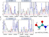 |
Fig. 2 Unblended or only slightly blended emission lines (red asterisks) of syn-HOCH2C(O)NH2 toward G358.93 MM1. Black lines show the observed spectra, while red lines represent the LTE model of syn-HOCH2C(O)NH2. Blue lines correspond to a composite model that includes contributions from all other identified molecular species. Dashed green lines mark the 3σ noise level. The upper-level energies (Eu) of the transitions are given above each panel. |
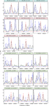 |
Fig. 3 Observed (gray) and best-fit LTE-modeled (red) spectra of NH2CHO, |

Molecular parameters derived from LTE fits using CLASS, and corresponding abundances relative to H2.
3.3 Spatial distribution
The spatial distributions of FA, AA, and GA were analyzed using the Cube Analysis and Rendering Tool for Astronomy (CARTA; Comrie et al. 2021). Only transitions verified to be free of significant blending were utilized to generate the integrated-intensity (moment-0) maps. As shown in Figs. 1c–e, the emissions of both FA and AA are nearly co-spatial with the 1 mm continuum peak of G358.93 MM1, consistent with previous findings for amide-bearing species (Duan et al. 2025b). The newly obtained GA map is compact and coincident with both the FA and AA emission peaks as well as the continuum maximum. The close morphological correspondence among all three amides indicates that they likely share related formation environments or interconnected chemical pathways in the hot-core region.
4 Discussion
4.1 Comparison with other sources and chemical models
To place the amide chemistry of HMC G358.93 MM1 in context, the derived molecular abundances and abundance ratios have been compared with those measured in other sources and with predictions from chemical models. All abundances are normalized to H2. The adopted N(H2) and its derivation are described in Appendix E. For reference, observational data were compiled for the molecular cloud G+0.693-0.027 (Rivilla et al. 2023; Zeng et al. 2023) and two HMCs: Sgr B2(N2) (Sanz-Novo et al. 2020; Belloche et al. 2017) and G31.41+0.41 (Colzi et al. 2021). Model predictions were drawn from Sahu et al. (2020) and Garrod et al. (2022).
Across all sources, a consistent abundance hierarchy is apparent: AA and FA are substantially more abundant than GA, while FA is typically comparable to or slightly higher than AA (Rivilla et al. 2023; Sanz-Novo et al. 2020; Colzi et al. 2021; Zeng et al. 2023; Belloche et al. 2017). G358.93 MM1 follows this overall ordering, although its FA/AA ratio lies toward the lower end of the hot-core distribution. In contrast, significantly higher values – such as FA/AA ≈ 25.8 in SgrB2(N2) (Belloche et al. 2017) – suggest that source-to-source variations reflect a combination of optical-depth effects, excitation temperature differences, beam dilution, and time-dependent chemistry along distinct warm-up tracks (Garrod et al. 2022). Despite these differences, the abundance ratios among FA, AA, and GA generally agree within an order of magnitude, suggesting that the underlying amide chemistry is broadly consistent across environments.
The most striking discrepancy arises for GA, whose observed abundance is systematically lower than predicted by current astrochemical models. While models (Sahu et al. 2020; Garrod et al. 2022) tend to produce GA at levels comparable to or exceeding AA, observations of both G358.93 MM1 and G+0.693-0.027 show it to be at least one order of magnitude lower than AA (this work and Rivilla et al. 2023). This tension likely reflects an overestimation of GA formation efficiency and/or an underrepresentation of its destruction processes in current networks – potentially due to optimistic diffusion barriers, incomplete treatment of OH- and H-abstraction reactions, or neglected photolytic pathways (Sahu et al. 2020; Garrod et al. 2022).
4.2 Chemical linkages of GA with FA and AA
Since the first detection of GA in G+0.693-0.027 (Rivilla et al. 2023), its chemical relationship to AA has been a central topic of discussion. Structurally, GA is the α-hydroxy derivative of AA (–CH3 → –CH2OH), naturally suggesting a shared formation network. GA can form via the OH + NH2COCH2 reaction, where the NH2COCH2 radical has been experimentally demonstrated to arise from H-abstraction at the methyl site of AA (Haupa et al. 2020). An alternative formation route proposed by Garrod et al. (2008) begins with H-abstraction from FA to produce the NH2CO radical, which then reacts with CH2OH to yield GA. These pathways collectively link GA formation to both FA and AA through common intermediate radicals.
Observationally, our ALMA data toward G358.93 MM1 are consistent with this precursor-based framework. Both AA and FA are substantially more abundant than GA (AA/GA∼16.6 and FA/GA∼32.3; Fig. 4), providing ample reservoirs of precursor radicals under warm-up conditions. Moreover, the close spatial correspondence among GA, AA, and FA (Fig. 1) further supports a shared chemical environment. The similarity of the FA/GA and AA/GA ratios of G358 MM1 and G+0.693-0.027 (Rivilla et al. 2023; Zeng et al. 2023) suggests that analogous amide-forming networks operate across both quiescent and hot-core regimes.
Nevertheless, with only two confirmed GA detections to date, any conclusions regarding its precise formation mechanisms remain preliminary. Expanded surveys targeting sources with different warm-up timescales, UV and cosmic-ray irradiation levels, and ice compositions – together with models that incorporate refined diffusion barriers, abstraction and destruction kinetics, and reactive-desorption efficiencies – will be crucial to constrain the chemical linkage of GA to FA and AA.
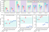 |
Fig. 4 (a) Abundances of FA, AA, and GA relative to H2 in G358.93 MM1, compared with other sources and model predictions. Model labels (1)= −(3) signify fast, medium, and slow warm-up models from Garrod et al. (2022), and (4) signifies the model of Sahu et al. (2020). (b–d) Abundance ratios FA/AA, AA/GA, and FA/GA. Arrows denote lower limits. The cyan-shaded regions indicate the uncertainty ranges (one order of magnitude) for the ratios derived in this work. |
5 Conclusions
We present the tentative detection of syn-glycolamide (syn-HOCH2C(O)NH2, GA) toward a HMC, G358.93–0.03 MM1, through seven unblended transitions with upper-level energies ranging from 108 to 389 K based on ALMA 1 mm data. Confirmation of this tentative identification will require future observations with a broader frequency coverage to reduce the likelihood of coincidental line blending in this line-rich source. The derived abundance of GA relative to H2 is (6.8±2.0)×10−11. In the same source, acetamide (CH3C(O)NH2, i.e., AA) and formamide (NH2CHO, i.e., FA) were also detected. The abundance ratios FA/GA and AA/GA in G358.93 MM1 closely resemble those measured in the molecular cloud G+0.693-0.027. These similarities suggest that related amide-forming networks operate in different environments, though the small number of GA detections precludes firm conclusions. Notably, current astrochemical models appear to overproduce GA, implying that its formation is overestimated and/or key destruction pathways are missing.
This detection extends the known occurrence of GA from Galactic center clouds to warm, dense protostellar environments, demonstrating that complex amides – and, by extension, amino acid precursors – can survive under the physical conditions characteristic of massive star formation. Continued laboratory, observational, and modeling efforts will be essential to constrain the formation routes and assess the broader astrochemical role of such species.
Data availability
The G358.93-0.03 data used in this paper are from ALMA. The raw dataset and documentation can be downloaded from https://almascience.nrao.edu/aq/. The derived data underlying this article are available in the article and in the supplementary material on Zenodo.
Acknowledgements
This work makes use of the following ALMA data: ADS/JAO.ALMA#2019.1.00768.S. ALMA is a partnership of ESO (representing its member states), NSF (USA), and NINS (Japan), together with NRC (Canada), MOST and ASIAA (Taiwan, China), and KASI (Republic of Korea), in cooperation with the Republic of Chile. The Joint ALMA Observatory is operated by ESO, AUI/NRAO, and NAOJ. We are grateful for support from the National SKA Program of China (No. 2025SKA0120100), National Natural Science Foundation of China (Grant No. W2512014), Fundamental Research Funds for the Central Universities (Grant No. 2025CDJ-IAISYB-060), and Postdoctoral Fellows Excellence Support Program (Grant No. 2404013554893087).
References
- Altwegg, K., Balsiger, H., Bar-Nun, A., et al. 2016, Sci. Adv., 2, e1600285 [NASA ADS] [CrossRef] [Google Scholar]
- Bakri, B., Demaison, J., Kleiner, I., et al. 2002, J. Mol. Spectrosc., 215, 312 [Google Scholar]
- Belloche, A., Meshcheryakov, A. A., Garrod, R. T., et al. 2017, A&A, 601, A49 [NASA ADS] [CrossRef] [EDP Sciences] [Google Scholar]
- Bergantini, A., Wang, J., Antonov, I., et al. 2025, ACS Central Science [Google Scholar]
- Blanco, S., López, J. C., Lesarri, A., & Alonso, J. L. 2006, J. Am. Chem. Soc., 128, 12111 [Google Scholar]
- Bonfand, M., Belloche, A., Garrod, R. T., et al. 2019, A&A, 628, A27 [NASA ADS] [CrossRef] [EDP Sciences] [Google Scholar]
- Brogan, C. L., Hunter, T. R., Towner, A. P. M., et al. 2019, ApJ, 881, L39 [NASA ADS] [CrossRef] [Google Scholar]
- Burton, A., Dworkin, J., Callahan, M., Glavin, D., & Elsila, J. 2012, in 39th COSPAR Scientific Assembly, 39, 264 [Google Scholar]
- Ceccarelli, C., Loinard, L., Castets, A., Faure, A., & Lefloch, B. 2000, A&A, 362, 1122 [Google Scholar]
- Chen, X., Sobolev, A. M., Ren, Z.-Y., et al. 2020, Nat. Astron., 4, 1170 [Google Scholar]
- Colzi, L., Rivilla, V. M., Beltrán, M. T., et al. 2021, A&A, 653, A129 [NASA ADS] [CrossRef] [EDP Sciences] [Google Scholar]
- Combes, F., Q-Rieu, N., & Wlodarczak, G. 1996, A&A, 308, 618 [NASA ADS] [Google Scholar]
- Comrie, A., Wang, K.-S., Hsu, S.-C., et al. 2021, CARTA: The Cube Analysis and Rendering Tool for Astronomy [Google Scholar]
- Cronin, J. R., & Pizzarello, S. 1983, Adv. Space Res., 3, 5 [Google Scholar]
- Cunningham, M. R., Jones, P. A., Godfrey, P. D., et al. 2007, MNRAS, 376, 1201 [NASA ADS] [CrossRef] [Google Scholar]
- Demyk, K., Wlodarczak, G., & Dartois, E. 2004, in SF2A-2004: Semaine de l’Astrophysique Francaise, eds. F. Combes, D. Barret, T. Contini, F. Meynadier, & L. Pagani, 493 [Google Scholar]
- Duan, C., Gou, Q., Liu, T., et al. 2025a, ApJ, 988, 95 [Google Scholar]
- Duan, C., Xu, X., Gou, Q., et al. 2025b, A&A, 702, A35 [NASA ADS] [CrossRef] [EDP Sciences] [Google Scholar]
- Gardner, F. F., Godfrey, P. D., & Williams, D. R. 1980, MNRAS, 193, 713 [Google Scholar]
- Garrod, R. T., Widicus Weaver, S. L., & Herbst, E. 2008, ApJ, 682, 283 [Google Scholar]
- Garrod, R. T., Jin, M., Matis, K. A., et al. 2022, ApJS, 259, 1 [NASA ADS] [CrossRef] [Google Scholar]
- Goldsmith, P. F., & Langer, W. D. 1999, ApJ, 517, 209 [Google Scholar]
- Haupa, K. A., Ong, W.-S., & Lee, Y.-P. 2020, Phys. Chem. Chem. Phys. (Incorp. Faraday Trans.), 22, 6192 [Google Scholar]
- Heineking, N., & Dreizler, H. 1993, Z. Naturf. A, 48, 787 [Google Scholar]
- Hirota, E., Sugisaki, R., Nielsen, C. J., & Sørensen, G. O. 1974, J. Mol. Spectrosc., 49, 251 [NASA ADS] [CrossRef] [Google Scholar]
- Ilyushin, V. V., Alekseev, E. A., Dyubko, S. F., Kleiner, I., & Hougen, J. T. 2004, J. Mol. Spectrosc., 227, 115 [Google Scholar]
- Ilyushin, V., Alekseev, E., Demaison, J., & Kleiner, I. 2006, J. Mol. Spectrosc., 240, 127 [Google Scholar]
- Jiménez-Serra, I., Vasyunin, A. I., Caselli, P., et al. 2016, ApJ, 830, L6 [Google Scholar]
- Jiménez-Serra, I., Martín-Pintado, J., Rivilla, V. M., et al. 2020, Astrobiology, 20, 1048 [Google Scholar]
- Jones, P. A., Cunningham, M. R., Godfrey, P. D., & Cragg, D. M. 2007, MNRAS, 374, 579 [NASA ADS] [CrossRef] [Google Scholar]
- Kauffmann, J., Bertoldi, F., Bourke, T. L., Evans, N. J., I., & Lee, C. W. 2008, A&A, 487, 993 [NASA ADS] [CrossRef] [EDP Sciences] [Google Scholar]
- Kojima, T., Yano, E., Nakagawa, K., & Tsunekawa, S. 1987, J. Mol. Spectrosc., 122, 408 [Google Scholar]
- Kryvda, A. V., Gerasimov, V. G., Dyubko, S. F., Alekseev, E. A., & Motiyenko, R. A. 2009, J. Mol. Spectrosc., 254, 28 [NASA ADS] [CrossRef] [Google Scholar]
- Kuan, Y.-J., Charnley, S. B., Huang, H.-C., Tseng, W.-L., & Kisiel, Z. 2003, ApJ, 593, 848 [NASA ADS] [CrossRef] [Google Scholar]
- Kukolich, S. G., & Nelson, A. C. 1971, Chem. Phys. Lett., 11, 383 [NASA ADS] [CrossRef] [Google Scholar]
- Liu, S.-Y., Girart, J., Remijan, A., & Snyder, L. 2002, ApJ, 576, 255 [NASA ADS] [CrossRef] [Google Scholar]
- Manna, A., & Pal, S. 2023, Ap & SS, 368, 33 [Google Scholar]
- Manna, A., & Pal, S. 2024, Res. Astron. Astrophys., 24, 075014 [Google Scholar]
- Manna, A., Pal, S., Viti, S., & Sinha, S. 2023, MNRAS, 525, 2229 [Google Scholar]
- Manna, A., Pal, S., & Viti, S. 2024, MNRAS, 533, 1143 [Google Scholar]
- Maret, S., Hily-Blant, P., Pety, J., Bardeau, S., & Reynier, E. 2011, A&A, 526, A47 [NASA ADS] [CrossRef] [EDP Sciences] [Google Scholar]
- Maris, A. 2004, Phys. Chem. Chem. Phys., 6, 2611 [CrossRef] [Google Scholar]
- Marstokk, K., & Mollendal, H. 1999, Acta Chem. Scand., 53, 79 [Google Scholar]
- McMullin, J. P., Waters, B., Schiebel, D., Young, W., & Golap, K. 2007, in Astronomical Society of the Pacific Conference Series, 376, Astronomical Data Analysis Software and Systems XVI, eds. R. A. Shaw, F. Hill, & D. J. Bell, 127 [NASA ADS] [Google Scholar]
- Millar, T. J. 2020, Chinese J. Chem. Phys., 33, 668 [NASA ADS] [CrossRef] [Google Scholar]
- Moskienko, E. M., & Diubko, S. F. 1991, Radiofizika, 34, 213 [Google Scholar]
- Motiyenko, R. A., & Margulès, L. 2025, A&A, 699, A348 [NASA ADS] [CrossRef] [EDP Sciences] [Google Scholar]
- Motiyenko, R. A., Tercero, B., Cernicharo, J., & Margulès, L. 2012, A&A, 548, A71 [NASA ADS] [CrossRef] [EDP Sciences] [Google Scholar]
- Müller, H. S. P., Thorwirth, S., Roth, D. A., & Winnewisser, G. 2001, A&A, 370, L49 [Google Scholar]
- Müller, H. S. P., Schlöder, F., Stutzki, J., & Winnewisser, G. 2005, J. Mol. Struct., 742, 215 [Google Scholar]
- Pearce, B. K. D., Tupper, A. S., Pudritz, R. E., & Higgs, P. G. 2018, Astrobiology, 18, 343 [Google Scholar]
- Perrero, J., Alessandrini, S., Ye, H., Puzzarini, C., & Rimola, A. 2025, A&A, 698, A51 [NASA ADS] [CrossRef] [EDP Sciences] [Google Scholar]
- Pickett, H. M., Poynter, R. L., Cohen, E. A., et al. 1998, J. Quant. Spec. Radiat. Transf., 60, 883 [Google Scholar]
- Pizzarello, S., & Weber, A. L. 2004, Science, 303, 1151 [Google Scholar]
- Potiszil, C., Ota, T., Yamanaka, M., et al. 2023, Nat. Commun., 14, 1482 [Google Scholar]
- Powell, M. J. D. 1964, Comput. J., 7, 155 [Google Scholar]
- Qin, S.-L., Wu, Y., Huang, M., et al. 2010, ApJ, 711, 399 [Google Scholar]
- Remijan, A., Snyder, L. E., Friedel, D. N., Liu, S.-Y., & Shah, R. Y. 2003, ApJ, 590, 314 [Google Scholar]
- Rivilla, V. M., Sanz-Novo, M., Jiménez-Serra, I., et al. 2023, ApJ, 953, L20 [NASA ADS] [CrossRef] [Google Scholar]
- Ruiz-Mirazo, K., Briones, C., & de la Escosura, A. 2014, Chem. Rev., 114, 285 [CrossRef] [Google Scholar]
- Sahu, D., Liu, S.-Y., Das, A., Garai, P., & Wakelam, V. 2020, ApJ, 899, 65 [NASA ADS] [CrossRef] [Google Scholar]
- Sánchez-Monge, Á., Schilke, P., Ginsburg, A., Cesaroni, R., & Schmiedeke, A. 2018, A&A, 609, A101 [Google Scholar]
- Sanz-Novo, M., Belloche, A., Alonso, J. L., et al. 2020, A&A, 639, A135 [NASA ADS] [CrossRef] [EDP Sciences] [Google Scholar]
- Sanz-Novo, M., Alonso, J. L., Rivilla, V. M., et al. 2022, A&A, 666, A134 [NASA ADS] [CrossRef] [EDP Sciences] [Google Scholar]
- Shimonishi, T., Izumi, N., Furuya, K., & Yasui, C. 2021, ApJ, 922, 206 [NASA ADS] [CrossRef] [Google Scholar]
- Snyder, L. E., Lovas, F. J., Hollis, J. M., et al. 2005, ApJ, 619, 914 [CrossRef] [Google Scholar]
- Suenram, R. D., Golubiatnikov, G. Y., Leonov, I. I., et al. 2001, J. Mol. Spectrosc., 208, 188 [NASA ADS] [CrossRef] [Google Scholar]
- Szőri, M., Jójárt, B., Izsák, R., et al. 2011, Phys. Chem. Chem. Phys. (Incorp. Faraday Trans.), 13, 7449 [Google Scholar]
- Vorob’eva, E. M., & Dyubko, S. F. 1994, Radiophys. Quant. Electron., 37, 155 [Google Scholar]
- Weber, A. L., & Pizzarello, S. 2006, PNAS, 103, 12713 [NASA ADS] [CrossRef] [Google Scholar]
- Wu, G. 2009, Amino Acids, 37, 1 [Google Scholar]
- Yamaguchi, A., Hagiwara, S., Odashima, H., Takagi, K., & Tsunekawa, S. 2002, J. Mol. Spectrosc., 215, 144 [Google Scholar]
- Yan, Y. T., Henkel, C., Kobayashi, C., et al. 2023, A&A, 670, A98 [NASA ADS] [CrossRef] [EDP Sciences] [Google Scholar]
- Zeng, S., Rivilla, V. M., Jiménez-Serra, I., et al. 2023, MNRAS, 523, 1448 [NASA ADS] [CrossRef] [Google Scholar]
Appendix A Spectroscopic line lists
Spectroscopic line lists used in this work were retrieved from the CDMS database. Table A.1 summarizes the catalogs entries, molecular identifiers, and the primary laboratory or theoretical studies on which each entry is based. Table A.2, only available on Zenodo, lists spectroscopic parameters of all unblended or minimally blended transitions analyzed in this work, including rest frequencies, upper-state energies (Eup), Einstein A-coefficients (Aij), degeneracies (gup), line width (∆V), and integrated intensity (∫TMBdv).
Spectroscopic data sources and references used in this work.
Appendix B The full source model of G358.93 MM1
To make sure that the spectral models are reliable, we added full source model fitting. All species in G358.93 MM1 have been included. The full source model is shown with a solid blue line in Fig. B.1. A complete list of all detected species is provided in Table B.1, together with the LTE parameters adopted for the full source model, including excitation temperature (Tex), column density (Nt), line width (full width at half maximum, FWHM), and velocity offset (Voff). For species other than GA, AA, and FA, these parameters were adjusted manually to best reproduce the observed spectrum. Figure B.1 and Table B.1 are available exclusively on Zenodo.
Appendix C The rotational diagram analysis for GA
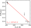 |
Fig. C.1 Rotational diagram of GA. Black points represent the observed data, while red lines indicate the best-fit results. The derived rotational temperature (Trot) is shown in the lower-left corner, with an assumed uncertainty of 20%. |
To verify the optimality of the fitting results from CLASS/ADJUST and the validity of the LTE assumption, we have made a rotational diagram analysis (Fig. C.1) using seven unblended transitions of GA. The rotational temperature and column density of a given species can be derived using the rotational diagram method, provided that multiple transitions covering distinct upper-level energies are available (e.g., Goldsmith & Langer 1999; Liu et al. 2002). Assuming LTE and optically thin emission, the level populations across different transitions can be characterized by a single rotational temperature. Additionally, under the assumption that the molecular emission completely fills the telescope beam, the beam-averaged column density and rotation temperature can be described by the following expression (Goldsmith & Langer 1999; Remijan et al. 2003; Qin et al. 2010):
 (C.1)
(C.1)
where Nu is the column density of the upper energy level, gup is upper level degeneracy, Nt is the total beam-averaged column density, Qrot is the rotational partition function, Eup is the upper level energy in K, k is the Boltzmann constant, Trot is the rotation temperature, v is the transition frequency, h is the Planck constant, c is the speed of light, Aul is the Einstein emission coefficient, ∫TMBdv is the integrated intensity of the specific transition.
The rotational diagram yields a rotational temperature of 107 ± 21 K. Considering the errors, the result agrees reasonably well with the value of 102 ± 20 K derived by the CLASS/ADJUST.
Appendix D STATCONT-based continuum subtraction and LTE modeling of GA
To address the potential impact of continuum subtraction on the identification of weak spectral features, we repeated the continuum subtraction using STATCONT (Sánchez-Monge et al. 2018), an automated tool designed to determine the continuum level in line-rich spectra without requiring manual selection of line-free channels. This analysis was performed to verify that our conclusions are not dependent on the specific continuum-subtraction method employed.
Figure D.1 presents a comparison between the spectra obtained with the CASA-based continuum subtraction and the STATCONT-based method, and can be found exclusively on Zenodo. The two spectra are nearly identical across the observed frequency ranges, demonstrating that our manual continuum subtraction procedure does not introduce systematic biases and that the identification of weak spectral features is robust against the choice of continuum-subtraction method.
Using the STATCONT-processed data, we re-identified the candidate GA transitions and performed LTE modeling following the same methodology described in the main text. Figure D.2 shows the unblended or only slightly blended emission lines (marked with red asterisks) of GA toward G358.93 MM1 identified in the STATCONT-based spectra, and is also available exclusively on Zenodo. Compared with the CASA-based analysis, the rms level in the STATCONT-based spectra is slightly higher (∼1.65 K), resulting in five lines detected above 3σ instead of six. Nevertheless, the same seven unblended candidate GA lines are recovered, and the derived column density and excitation temperature – N = (3.7 ± 0.7) × 1014 cm−2 and Tex = 98 ± 20 K – are consistent with those obtained from the CASA-based analysis within the adopted uncertainties. Notably, the column density derived from the STATCONT-based analysis is approximately 30% lower than that from the CASA-based analysis (5.3 × 1014 cm−2). This comparison shows that, although the derived column density is somewhat method-dependent, our conclusions regarding the tentative identification of GA is not driven by the particular continuum-subtraction approach adopted.
Appendix E H2 column density from the dust continuum
We estimated the molecular hydrogen column density,  , from the 1 mm dust continuum emission under the standard assumption of optically thin thermal dust emission. The beam-averaged column density was calculated using the following relation (e.g., Maret et al. 2011; Bonfand et al. 2019):
 (E.1)
(E.1)
where Sν is the integrated continuum flux density within the extraction beam, Rgd = 100 is the gas-to-dust mass ratio, µ = 2.8 is the mean molecular weight per H2 molecule (Kauffmann et al. 2008), mH is the mass of hydrogen atom, Ω is the beam solid angle, κν is the dust opacity, and Bν(Tdust) is the Planck function evaluated at the dust temperature Tdust. We adopt κν = 2 cm2 g−1 at λ∼1 mm (Bonfand et al. 2019) and Tdust = 150 K, following Chen et al. (2020). With these assumptions, we derive  for G358.93 MM1, where a conservative uncertainty of 20% is assumed. Molecular abundances relative to H2 were then calculated as
  , and the resulting χ values are reported in Table 1.
All Tables
Molecular parameters derived from LTE fits using CLASS, and corresponding abundances relative to H2.
All Figures
|
Fig. 1 (a) 1 mm continuum image of G358.93-0.03. Contour levels correspond to (20, 40, 80, 120, 200, 500, 1000, 1700) × σ, where σ is the rms noise level. The white ellipse in the lower-left corner indicates the synthesized beam of 0.15″×0.1″ (position angle –87.1◦). (b) Enlarged view of G358.93 MM1. The continuum peak is marked by a white cross, and the offset extraction position used for spectral analysis is marked by a red cross. (c–e) Integrated intensity (moment-0) maps of NH2CHO, CH3C(O)NH2, and syn-HOCH2C(O)NH2 toward G358.93 MM1, overlaid with the 1 mm continuum emission contours from panel (a). The color scale unit is Jy beam−1 km s−1. |
| In the text | |
|
Fig. 2 Unblended or only slightly blended emission lines (red asterisks) of syn-HOCH2C(O)NH2 toward G358.93 MM1. Black lines show the observed spectra, while red lines represent the LTE model of syn-HOCH2C(O)NH2. Blue lines correspond to a composite model that includes contributions from all other identified molecular species. Dashed green lines mark the 3σ noise level. The upper-level energies (Eu) of the transitions are given above each panel. |
| In the text | |
|
Fig. 3 Observed (gray) and best-fit LTE-modeled (red) spectra of NH2CHO, |
| In the text | |
|
Fig. 4 (a) Abundances of FA, AA, and GA relative to H2 in G358.93 MM1, compared with other sources and model predictions. Model labels (1)= −(3) signify fast, medium, and slow warm-up models from Garrod et al. (2022), and (4) signifies the model of Sahu et al. (2020). (b–d) Abundance ratios FA/AA, AA/GA, and FA/GA. Arrows denote lower limits. The cyan-shaded regions indicate the uncertainty ranges (one order of magnitude) for the ratios derived in this work. |
| In the text | |
|
Fig. C.1 Rotational diagram of GA. Black points represent the observed data, while red lines indicate the best-fit results. The derived rotational temperature (Trot) is shown in the lower-left corner, with an assumed uncertainty of 20%. |
| In the text | |
Current usage metrics show cumulative count of Article Views (full-text article views including HTML views, PDF and ePub downloads, according to the available data) and Abstracts Views on Vision4Press platform.
Data correspond to usage on the plateform after 2015. The current usage metrics is available 48-96 hours after online publication and is updated daily on week days.
Initial download of the metrics may take a while.