


| Issue |
A&A
Volume 709, May 2026
|
|
|---|---|---|
| Article Number | A278 | |
| Number of page(s) | 19 | |
| Section | Planets, planetary systems, and small bodies | |
| DOI | https://doi.org/10.1051/0004-6361/202658974 | |
| Published online | 25 May 2026 | |
The spin state of asteroid Apophis and a prediction of its change during the 2029 close encounter with Earth
1
Charles University, Faculty of Mathematics and Physics, Institute of Astronomy,
V Holešovičkách 2,
180 00
Prague,
Czech Republic
2
Astronomical Institute of the Czech Academy of Sciences,
Fričova 298,
251 65
Ondřejov,
Czech Republic
3
Florida Space Institute, University of Central Florida,
12354 Research Parkway, Partnership 1 building,
Orlando,
FL,
32828,
USA
4
Space sciences, Technologies and Astrophysics Research Institute, Université de Liège,
Allée du 6 Aoút 17,
4000
Liège,
Belgium
5
Department of Applied Physics and Astronomy, and Sharjah Space and Astronomy Hub, University of Sharjah,
United Arab Emirates
6
Technische Universitaet Braunschweig, Institute of Geophysics and Extraterrestrial Physics,
Braunschweig,
Germany
7
Faculty of Physics, Weizmann Institute of Science,
Rehovot
0076100,
Israel
8
European Southern Observatory,
Alonso de Córdova 3107, Vitacura, Casilla
19001,
Santiago,
Chile
9
Department of Earth, Atmospheric, and Planetary Sciences, Massachusetts Institute of Technology,
77 Massachusetts Avenue,
Cambridge,
MA
02139,
USA
10
Astronomical Observatory Institute, Faculty of Physics and Astronomy, Adam Mickiewicz University,
Słoneczna 36,
60-286
Poznań,
Poland
11
Astronomical Observatory, Jagiellonian University,
ul. Orla 171,
30-244
Krakow,
Poland
12
Mt. Suhora Astronomical Observatory, University of the National Education Commission,
ul. Podchorazych 2,
30-084
Krakow,
Poland
13
Janusz Gil Institute of Astronomy, University of Zielona Góra,
Lubuska 2,
65-265
Zielona Góra,
Poland
14
Université Côte d’Azur, CNRS-Lagrange, Observatoire de la Côte d’Azur,
CS 34229,
06304
Nice Cedex 4,
France
15
Department of Physics and Astronomy, University of North Carolina at Chapel Hill,
Chapel Hill,
NC
27599,
USA
16
Oukaimeden Observatory, High Energy Physics, Astrophysics and Geoscience Laboratory, Faculté des Sciences Semlalia (FSSM), Cadi Ayyad University,
Marrakesh,
Morocco
★ Corresponding author: This email address is being protected from spambots. You need JavaScript enabled to view it.
Received:
15
January
2026
Accepted:
15
April
2026
Abstract
Context. On April 13, 2029, the asteroid Apophis will pass near Earth at a geocentric distance of about 38 000 km. This will provide a unique opportunity to study the effects of Earth’s gravitational torque on the asteroid’s spin state and figure. Numerical models have suggested that the post-encounter spin state will critically depend on the orientation of Apophis during the flyby.
Aims. We aim to determine the spin state of Apophis from its photometric observations collected during two apparitions in 2012–2013 and 2020–2021. This will enable us to accurately predict the pre-encounter rotation state and, by accounting for Earth’s gravitational torque, predict a range of possible post-encounter states.
Methods. We used the light curve inversion method for tumbling asteroids to reconstruct the spin state of Apophis and its convex shape model. The result is adopted as the initial condition of a numerical model describing Apophis’s future rotation state.
Results. The data from the two apparitions are insufficient to determine Apophis’s rotation and precession periods uniquely. The formally best-fit solution is Pϕ = 27.374 ± 0.001 h for the precession period and Pψ = 262.2 ± 0.1 h for the rotation period, but at least two other combinations of the periods provide a similarly good fit to the available data. All the currently acceptable models result in approximately the same pre-encounter orientation of Apophis in early 2029 (within 20° in terms of Euler angles). This is because the accurate photometric data were collected during two apparitions separated by 8 years, which is the same interval as from 2021 to 2029. Although the close encounter with Earth in April 2029 hugely increases the post-encounter uncertainty of Apophis’s spin state, the short-axis spin mode will be preserved with a high likelihood.
Conclusions. Additional observations taken in 2027 and 2028 will break the ambiguity in Apophis’s pre-encounter spin solution and allow us to get a more accurate post-encounter spin state prediction.
Key words: minor planets, asteroids: general / minor planets, asteroids: individual: (99942) Apophis
© The Authors 2026
 Open Access article, published by EDP Sciences, under the terms of the Creative Commons Attribution License (https://creativecommons.org/licenses/by/4.0), which permits unrestricted use, distribution, and reproduction in any medium, provided the original work is properly cited.
This article is published in open access under the Subscribe to Open model. This email address is being protected from spambots. You need JavaScript enabled to view it. to support open access publication.
1 Introduction
The asteroid (99942) Apophis is a near-Earth object classified as a potentially hazardous asteroid. It received significant attention after reaching the Torino scale of 4 for a few days in late 2004. The probability of Apophis impacting Earth in April 2029 quickly dropped with further observations, but its very close approach to Earth, which is predicted to occur on April 13, 2029, is still a rare event for a body of this size (Brož et al. 2026). Physically, Apophis is characterized as an Sq-class asteroid (Binzel et al. 2009) with a mean diameter of about 340–420 m (Müller et al. 2014; Licandro et al. 2016; Brozović et al. 2018; Brož et al. 2026), slowly rotating in an excited rotation state (Pravec et al. 2014; Lee et al. 2022). A significant amount of effort has been devoted to precisely determining its orbit and future impact probabilities (Farnocchia et al. 2013; Vokrouhlický et al. 2015b).
Its upcoming encounter with Earth on April 13, 2029, presents a great scientific opportunity to study this object and promote the importance of planetary defense (Reddy et al. 2022). One key scientific aspect of the flyby is that Earth’s gravitational torques will alter Apophis’s rotational state (Benson et al. 2023). The exact outcome depends on Apophis’s attitude during the flyby and its tensor of inertia. Possible tidally driven surface movement depends on the interior and regolith structure (Yu et al. 2014). In general, this unique natural experiment can be used to extract information about Apophis’s interior that would otherwise be inaccessible. There are at least three space missions planned to explore Apophis: OSIRIS-APEX, the NASA mission that will start proximity operation after the encounter (DellaGiustina et al. 2023; Nolan et al. 2025); the ESA mission RAMSES that will rendezvous with Apophis even before it passes Earth (Lazzarin et al. 2025; Michel et al. 2025); and DESTINY+, the JAXA mission that is planned to fly by Apophis in February 2029 (Arai & Destiny+ Team 2025). Although Apophis will be studied in detail before and after it encounters Earth, to maximize the scientific output from the post-encounter observations, Apophis’s pre-encounter properties must be known. In particular, its spin state will change during its flyby towards Earth, so the information about the pre-encounter spin state is critical to any interpretation of how the spin would be affected. Moreover, knowing the spin state precisely will enable us to predict the flyby attitude, compute the effects of torques, and indicate the post-encounter spin state, which is essential for proximity operations of spacecraft.
This paper aims to use photometric data of Apophis (Section 2) to reconstruct its shape and spin model (Section 3). From this model, we predicted its post-encounter spin state (Section 4).
2 Photometric data
Apophis was discovered in June 2004. The first photometric data came from January 2005 (V. Reddy) and are available at the Asteroid Lightcurve Photometry Database1. However, the data do not contain much information about Apophis’s rotation, as they are only differential magnitudes and cover only three nights.
Other data from the same apparition are presented on the web page of R. Behrend2. They are also only relative; see the discussion by Pravec et al. (2014).
During the next favorable apparition of Apophis in 2012–2013, Pravec et al. (2014) took an extensive photometric dataset covering an interval from December 2012 to April 2013 and found that Apophis is an excited (tumbling) spin state. They constructed a convex shape model of Apophis, with the precession period Pϕ = 27.38 ± 0.02 h and the rotation period Pψ = 263 ± 2 h in the Kaasalainen (2001) convention. This model agreed with radar delay-Doppler observations from the same apparition. From the radar observations, a few possible non-convex shape models were constructed (Brozović et al. 2018).
Many observers have used the latest observing window of Apophis in 2020–2021 to obtain more photometric data. We conducted observations with the 1.54m Danish telescope at the La Silla Observatory in Chile from November 16, 2020, to May 6, 2021. The telescope (IAU/MPC code W74) is equipped with a 2048 × 2048 px CCD detector with a pixel size of 13.5 μm. This configuration provides a plate scale of 0.40 arcsec2 pixel−1 and a field of view of 13.5 × 13.5 arcmin2. We observed Apophis on 67 individual nights, collected 1280 data points calibrated in the Cousins R photometric system, covering a phase angle range of 24–100° (Table A.1). The telescope was tracked at half of the apparent sky motion rate of the asteroid. We processed and photometrically reduced the observations using our standard procedure as described in Pravec et al. (2014), Fatka et al. (2025), and the references therein. The absolute accuracy of the Cousins R calibrations using the Landolt (1992) standard stars was 0.01 mag, which makes it a unique dataset when compared with other photometric light curve datasets that we used as relative data, as described below.
We initially adopted Transiting Exoplanet Survey Satellite (TESS; Ricker et al. 2015) photometric data of Apophis from Sector 35, spanning February 19 to March 7, 2021, as reported by Lee et al. (2022) and processed following the scheme of Pál et al. (2020). While these data were incorporated into our analysis, our initial shape modeling revealed significant inconsistencies between the best-fitting solution and the TESS light curves, in contrast to the good agreement obtained with other datasets. To investigate this issue, we independently extracted the TESS photometry using the pipeline developed by Humes & Hanuš (2024). Apophis was observed with two detectors (CCD 1 of Camera 1 and CCD 1 of Camera 2). The Camera 2 dataset contains a ~4-day gap, during which we discarded anomalous points that showed imperfect background subtraction. According to the Sector 35 release notes3 (Fausnaugh et al. 2021), TESS lost fine pointing during this interval. Since our reduction does not include an additional alignment step on the backgroundsubtracted frames, the affected measurements are unreliable and were excluded from further analysis. The dataset obtained using the Humes & Hanuš (2024) pipeline performed significantly better in shape modeling (Sect. 3.1), and we therefore adopted it in place of the data from Lee et al. (2022).
We used time-series photometry of Apophis with the two TRAPPIST 0.6-m robotic telescopes – TRAPPIST-South at ESO La Silla, Chile (TS) and TRAPPIST-North at the Oukaimeden Observatory, Morocco (TN) – on multiple nights between January 15 and April 13, 2021 (see Table A.2). The twin Ritchey–Chrétien systems are operated remotely from Liège and designed for high-precision CCD photometry. All observations were conducted with the wide Exo filter, and the instrumental magnitudes were calibrated against field stars to the Cousins R system. For technical descriptions of the facilities, see Jehin et al. (2011).
We utilized photometric observations of Apophis from Reddy et al. (2022) obtained with the 0.7-m telescope at the Wise Observatory, Israel, over 15 nights between December 24, 2020, and April 7, 2021. All images were acquired using a wide Luminance filter, and the photometry from each night was relatively calibrated against nearby field stars (Polishook & Aharonson 2020).
Furthermore, we obtained lightcurve data of Apophis during five nights at the Observatoire du Mont-Mégantic (OMM) in Québec, Canada. The observatory operates a 1.6-m Ritchey–Chrétien telescope equipped with two CCD cameras. We used the PESTO instrument with the Sloan photometric filters.
We also utilized photometric data collected by Lee et al. (2022) from various sources, kindly provided by the first author. Their dataset consists of more than 200 light curves observed with 36 telescopes.
Other photometric data were obtained by observers participating in the Gaia-GOSA project (Santana-Ros et al. 2016) and by individual professional observers. In particular, we used (i) the 1.54 m reflecting telescope located at the Estación Astrofísica de Bosque Alegre (EABA, MPC code 821) situated in the Sierras Chicas, Córdoba, Argentina; (ii) the 0.7 m Roman Baranowski Telescope (RBT/PST2) of the Adam Mickiewicz University located at the Winer Observatory in Arizona, USA; (iii) the Panchromatic Robotic Optical Monitoring and Polarimetry Telescopes (PROMPT) built by the University of North Carolina at Cerro Tololo Inter-American Observatory (CTIO) in Chile (Zola et al. 2021); (iv) the 0.6 m Cassegrain telescope at the Mount Suhora Observatory in Poland; (v) the 0.6 m telescope at the Adiyaman University Application and Research Center in Adiyaman, Turkey; and (vi) the 0.5 m OAUJ-CDK500 telescope (Zola et al. 2025) of the Astronomical Observatory of the Jagiellonian University. The data are listed in Table A.2.
3 Determining the spin state
Because of Apophis’s excited rotation, the shape and spin state reconstruction from photometric data is more complicated than in the case of a principal axis rotator. The method of light curve inversion for tumbling asteroids was developed by Kaasalainen (2001), and we used the same formalism here. The spin state is described by the angular momentum vector L; initial orientation defined by three Euler angles (ϕ0, θ0, ψ0) of precession, nutation, and rotation, respectively; and normalized principal axes I1, I2 of the inertia tensor (with I3 = 1). For practical reasons of the inversion method, the four parameters L and θ0 were substituted with an equivalent set of parameters that are the direction of the angular momentum vector in ecliptic coordinates (λ, β), the rotation period Pψ, and the precession period Pϕ. The details and other relevant references can be found in the Appendix of Kaasalainen (2001). The asteroid’s shape was modeled as a convex polyhedron with facet areas approximated by a series of harmonic functions. Coefficients of the series thus represent shape model parameters (Kaasalainen & Torppa 2001). The order and degree of the harmonic expansion were eight, so the total number of shape parameters was 80 because the zero-order parameter corresponds to the size, which is not constrained in our model. The algorithm starts from initial parameter values and converges to a local minimum in the standard χ2 metric.
This method of light curve inversion was already used on Apophis by Pravec et al. (2014) and Lee et al. (2022). The model by Pravec et al. (2014) was constructed from only one apparition data, so the uncertainties of the determined spin parameters, namely the rotation and precession periods, were relatively large and do not allow predictions of Apophis’s orientation in 2029 to be made. To accurately predict the orientation of Apophis in 2029, we needed to know the periods precisely; therefore, using data from both apparitions, 2012–2013 and 2020–2021, was necessary. The formal uncertainties of the model constructed by Lee et al. (2022) are small enough for extrapolation to 2029, but, as we demonstrate below, there are also other spin solutions present that provide the same or even better fits than the model made by Lee et al. (2022). In this context, analyzing the uniqueness of the light curve inversion solution and providing a realistic estimation of the model uncertainties is critical.
The available photometric dataset is huge and heterogeneous. To speed up the computations and ensure that systematic errors would not affect our solution, we selected only the most accurate data subset: the data taken with the 1.54 m Danish telescope (DK154) in 2012–2013 (158 points) and 2020–2021 (1280 points), and the TESS data (1149 points). For the 2020–2021 apparition, the DK154 dataset is the most homogeneous, and it covers the widest interval of geometries (Table A.1), while the TESS data almost continuously cover the longest time interval of about 15 days.
Although the data from different observatories vary in their photometric accuracy, we did not take this into account and used all data points with the same weights. This simplified approach is justified because the introduced error is much smaller than the errors caused by systematic effects and the ambiguity in the spin solution. Different weights would affect the model parameters on the same order as the difference between models A and A* described in the next section.
3.1 Multiple solutions
To ensure we do not miss the global minimum in χ2, we initiated the inversion over a grid of initial spin parameters centered around the values estimated in the previous works. The algorithm then converged to a local minimum in χ2. The most critical parameters are the two periods; their scan is shown in Fig. 1. For each pair of initial Pϕ, Pψ, we optimized all eight spin parameters, the shape, and Hapke’s scattering parameters. There are several local minima with significantly different periods but having almost the same values of root mean square (RMS) residuals. We selected the 20 best local minima and ran a higher resolution inversion model with more iterations to further improve the fit. This resulted in eight models (listed in Table 1) whose periods are marked as dotted lines in Fig. 1, and the lower residuals are marked as red asterisks. The plots show a clear pattern of local minima that are separated by ΔPϕ = 0.0106 h and ΔPψ = 0.969 h. Figure 2 shows the same data, but now the RMS values are color-coded and the correlation between periods is seen. The three groups of the best local minima are denoted A, B, and C. Their separation is such that over 8 years that separate the apparitions 2012–2013 and 2020–2021, there are n cycles of Pϕ and m cycles of Pψ, where n ≈ 2560 and m ≈ 270. All acceptable period pairs follow the relation ![Mathematical equation: $\[(P_{\phi}^{-1}-P_{\psi}^{-1})^{-1}=30.5658 \mathrm{~h}\]$](/articles/aa/full_html/2026/05/aa58974-26/aa58974-26-eq1.png) , which is the main period of Apophis’s light curve (Pravec et al. 2014). Solution B corresponds to n + 1 and m + 1 cycles, while solution C corresponds to n − 1 and m − 1 cycles. Because the photometric data can be fitted about equally well with all three combinations of periods, we cannot uniquely determine the number of cycles that elapsed from 2013 to 2020.
, which is the main period of Apophis’s light curve (Pravec et al. 2014). Solution B corresponds to n + 1 and m + 1 cycles, while solution C corresponds to n − 1 and m − 1 cycles. Because the photometric data can be fitted about equally well with all three combinations of periods, we cannot uniquely determine the number of cycles that elapsed from 2013 to 2020.
An interesting feature of this degeneracy is that all three models predict a similar orientation of Apophis in 2029, because the separation between 2013 and 2021 is eight years, which is also the separation between 2021 and 2029. As shown in Fig. 3, the Euler angles that define the orientation of the body in space are similar for the three models in 2013 and 2021, which is not surprising because the models were derived from observations in these two apparitions. The orientation of these models between and outside the two apparitions is different, which means that we cannot determine it uniquely. However, after another interval of 8 years, the different solutions again give about the same orientation of Apophis. This means that we can predict, at least to some level of precision, the orientation of Apophis during its 2029 encounter. On the other hand, this also means that photometric observations from 2029 cannot effectively distinguish between models A, B, and C. The difference between Euler angles for the three models in April 2029 is ~20° in ϕ, ~5° in θ, and ~5° in ψ. However, as we show in Sect. 4, the post-encounter spin state is very sensitive to the exact orientation of Apophis, so this accuracy is not sufficient to predict it precisely.
The shape model corresponding to solution A is shown in Fig. 4. It is formally the best solution with the lowest RMS residuals. In the same figure, we also show the shape model (called A*) constructed from the full set of photometric data. The visual difference between shape A and A* is about the same as between models A and B or C. Shape models A, A′, and A″ are practically the same. Figures B.1 and B.2 show how the model fits the photometric data from 2012–2013 and 2020–2021, respectively. The complete spin parameters are listed in Table 2. The shapes are similar, with minor differences that demonstrate the effect of different datasets on the shape details. We remind the reader that the shape model is convex and that the real shape of Apophis can contain concavities that cannot be reconstructed from the disk-integrated photometry. A bifurcated shape was suggested for Apophis by Brozović et al. (2018) based on the bifurcation seen in radar delay-Doppler images taken in 2013. Also, the spin parameters of models A and A* are similar; their differences are order-of-magnitude estimates of the uncertainty caused by the differences between the input datasets. However, both models represent only one local minimum in period parameter space. If we take the spread of periods for models A, A′, and A″ as the estimate of the real periods uncertainty, then the parameters for the best-fit model are Pϕ = 27.374 ± 0.001 h and Pψ = 262.2 ± 0.1 h. The uncertainty intervals are more than one order of magnitude smaller than those of Pravec et al. (2014) (due to the much larger time span of our dataset), and they overlap. On the contrary, values reported by Lee et al. (2022) have an order of magnitude smaller formal uncertainties, and they are outside our intervals for both periods. Lee et al. (2022) estimated the uncertainties from χ2 confidence intervals, which likely correspond to formal errors inside local minima, not to realistic uncertainties over a wider parameter space.
The error in the direction of the angular momentum vector can be estimated from the standard deviation of red points in Fig. 8, which is 10° in the ecliptic latitude λ and 0.7° in the ecliptic latitude β. The uncertainty of λ seems large, but this is just the effect of spherical coordinates and the β value being close to −90°. After correcting by cos β, the uncertainty in the longitudinal direction becomes 0.6°, which means that the direction of the angular momentum vector is known with a precision of about 1°. However, this formal uncertainty does not take into account the effect of regular precession caused by the solar gravitational torque (Sect. 4.2.1). As is apparent from the difference between β values for models A and A* in Table 2, the real uncertainty of the direction of L is at least a few degrees.
Apart from the uncertainty of the periods, there is also a considerable uncertainty of the moments of inertia I1, I2. There is some spread in these values in Table 1, but the realistic uncertainty is much larger. Periods can be determined precisely (although not uniquely) because they affect the phase of the light curve, which can be determined precisely from observations. On the contrary, moments of inertia primarily affect the shape of the light curve, which is not fully captured by the data, especially at the beginning and the end of the observing window (Fig. B.2), where the light curve sampling is sparse (as the observability of Apophis with ground-based telescopes was limited near the beginning and end of the apparitions). Thus, different combinations of moments of inertia produce slightly different model light curves that still agree with the data. We tested wide intervals of I1, I2, and by assessing how well the synthetic data agreed with the observed data, we roughly estimated the range of possible values as 0.45–0.65 for I1 and 0.965–0.985 for I2, with negative correlation between the parameters.
Although the parameter I1 is only poorly constrained directly by the model, it is constrained indirectly by the requirement that the kinematic parameters I1, I2 are consistent with principal moments of inertia ![Mathematical equation: $\[I_{1,2}^{\mathrm{sh}}\]$](/articles/aa/full_html/2026/05/aa58974-26/aa58974-26-eq3.png) computed ex post from the reconstructed 3D shape model assuming uniform density. Values of
computed ex post from the reconstructed 3D shape model assuming uniform density. Values of ![Mathematical equation: $\[I_{1}^{\text {sh}}\]$](/articles/aa/full_html/2026/05/aa58974-26/aa58974-26-eq4.png) for models A and A* are given in Table 2. They are around 0.6, which is consistent with the range of values from the fitting. Changing
for models A and A* are given in Table 2. They are around 0.6, which is consistent with the range of values from the fitting. Changing ![Mathematical equation: $\[I_{1}^{\text {sh}}\]$](/articles/aa/full_html/2026/05/aa58974-26/aa58974-26-eq5.png) to 0.5, for example, would require stretching the shape along the longest axis by about 15%, which would affect the lightcurves significantly. On the other hand,
to 0.5, for example, would require stretching the shape along the longest axis by about 15%, which would affect the lightcurves significantly. On the other hand, ![Mathematical equation: $\[I_{2}^{\text {sh}}\]$](/articles/aa/full_html/2026/05/aa58974-26/aa58974-26-eq6.png) of 0.91 is far outside the uncertainty interval of I1, but bringing it to 0.965 requires less dramatic change of the middle principal axis of about 8%. However, even this shape deformation would clearly deteriorate the light curve fit. Because the 3D shape is not known during the optimization, the shape-dependent parameters
of 0.91 is far outside the uncertainty interval of I1, but bringing it to 0.965 requires less dramatic change of the middle principal axis of about 8%. However, even this shape deformation would clearly deteriorate the light curve fit. Because the 3D shape is not known during the optimization, the shape-dependent parameters ![Mathematical equation: $\[I_{1,2}^{\mathrm{sh}}\]$](/articles/aa/full_html/2026/05/aa58974-26/aa58974-26-eq7.png) must be computed after the optimization, serving as a consistency check. Perfect match between I1,2 and
must be computed after the optimization, serving as a consistency check. Perfect match between I1,2 and ![Mathematical equation: $\[I_{1,2}^{\mathrm{sh}}\]$](/articles/aa/full_html/2026/05/aa58974-26/aa58974-26-eq8.png) cannot be expected because the convex model inevitably differs in moments of inertia from the real, yet unknown, shape of Apophis.
cannot be expected because the convex model inevitably differs in moments of inertia from the real, yet unknown, shape of Apophis.
 |
Fig. 1 Period scan. The plots show the residuals (blue points) of the fit for different values of the precession period Pϕ (left) and the rotation period Pψ (right). The dotted vertical lines indicate the positions of the eight best solutions, and the red crosses represent RMS residuals for the high-resolution models. The distances between local minima ΔPϕ and ΔPψ are denoted. |
Best models.
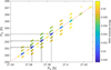 |
Fig. 2 Period scan. The plot shows the same data as in Fig. 1, but here the RMS residuals are color coded, and both the precession period Pϕ and rotation period Pψ are plotted to visualize the correlation between them. The best solutions with the lowest residuals (blue color) lie on the red dashed line that is in fact part of a hyperbola satisfying the relation |
![Mathematical equation: $\[(P_{\phi}^{-1}-P_{\psi}^{-1})^{-1}=30.5658 \mathrm{~h}\]$](/articles/aa/full_html/2026/05/aa58974-26/aa58974-26-eq2.png)
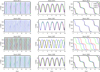 |
Fig. 3 Evolution of Euler angles for models A (blue), B (red), and C (green). The plots show the evolution of Euler angles ϕ, θ, and ψ within a month in different years. All three angles are similar for all three models in the years 2013, 2021, and 2029 because they are separated by 8 years. The Euler angles, and thus the orientation of the models, differ for epochs between these years (e.g., March 2027). |
3.2 Light scattering model
To properly model how the brightness of Apophis changes with rotation and changing illumination and viewing geometry, we used Hapke’s scattering model (Hapke 2012) with parameters w, g, h, B0, ![Mathematical equation: $\[\bar{\theta}\]$](/articles/aa/full_html/2026/05/aa58974-26/aa58974-26-eq9.png) . Because the observations did not cover phase angles below ~20°, the parameters h and B0 describing the width and amplitude of the opposition effect were fixed at the values for an average S-type asteroid, namely h = 0.08, B0 = 1.6 (Helfenstein & Veverka 1989; Li et al. 2015)4. Although the observations cover phase angles up to 100°, the disk-integrated photometry without albedo information does not allow the parameters of Hapke to be constrained. The only parameter that could be reasonably constrained was macroscopic roughness
. Because the observations did not cover phase angles below ~20°, the parameters h and B0 describing the width and amplitude of the opposition effect were fixed at the values for an average S-type asteroid, namely h = 0.08, B0 = 1.6 (Helfenstein & Veverka 1989; Li et al. 2015)4. Although the observations cover phase angles up to 100°, the disk-integrated photometry without albedo information does not allow the parameters of Hapke to be constrained. The only parameter that could be reasonably constrained was macroscopic roughness ![Mathematical equation: $\[\bar{\theta}\]$](/articles/aa/full_html/2026/05/aa58974-26/aa58974-26-eq10.png) . The values of
. The values of ![Mathematical equation: $\[\bar{\theta}\]$](/articles/aa/full_html/2026/05/aa58974-26/aa58974-26-eq11.png) between 30 and 35 degrees provided the best fit. Parameters w (single-scattering albedo) and g (asymmetry factor) were constrained only poorly to intervals 0.25–0.45 and −0.3 to −0.2, respectively. The best-fit set of parameters is: w = 0.42, h = 0.08, B0 = 0.94, g = −0.25, and
between 30 and 35 degrees provided the best fit. Parameters w (single-scattering albedo) and g (asymmetry factor) were constrained only poorly to intervals 0.25–0.45 and −0.3 to −0.2, respectively. The best-fit set of parameters is: w = 0.42, h = 0.08, B0 = 0.94, g = −0.25, and ![Mathematical equation: $\[\bar{\theta}\]$](/articles/aa/full_html/2026/05/aa58974-26/aa58974-26-eq12.png) = 33°. The geometric albedo p is uniquely defined by Hapke’s parameters. The values above yield p = 0.24, which agrees with the value 0.35 ± 0.10 based on the radar shape model (Brozović et al. 2018) or the range 0.24–0.33 derived from thermal infrared observations (Licandro et al. 2016). However, due to the wide range of acceptable Hapke parameters, the range of albedo values is also large, spanning between 0.16 and 0.28.
= 33°. The geometric albedo p is uniquely defined by Hapke’s parameters. The values above yield p = 0.24, which agrees with the value 0.35 ± 0.10 based on the radar shape model (Brozović et al. 2018) or the range 0.24–0.33 derived from thermal infrared observations (Licandro et al. 2016). However, due to the wide range of acceptable Hapke parameters, the range of albedo values is also large, spanning between 0.16 and 0.28.
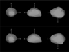 |
Fig. 4 Best models A (top) and A* (bottom) with parameters listed in Table 2. Model A was constructed from a subset of accurately calibrated photometry from the Danish telescope (La Silla) and TESS observations, while for model A*, we used all available photometry. |
Nominal models.
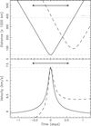 |
Fig. 5 Parameters of the Apophis close encounter with Earth on April 13, 2029. The top panel shows the geocentric (solid line) and selenocentric (dashed line) distance, and the bottom panel shows the relative geocentric and selenocentric velocity. The origin of the abscissa is at the nominal Earth closest approach epoch 62239.90709 (MJD). The horizontal dashed line at the top panel indicates the closest approach distance of 38 012 km, the horizontal dashed lines at the bottom panel show the relative geocentric velocities at the closest approach, 7.42 km s−1, and the asymptotic value, 5.84 km s−1. The closest approach to the Moon is at 95 959 km. The black arrow shows the Apophis Pϕ timescale for reference. |
4 Apophis’s change in spin state during its close approach to Earth in April 2029
The unusually close approach of the few-hundred-meter sized asteroid Apophis to Earth in April 2029 presents a rather rare event in asteroid science (Fig. 5). Not only will it continue to serve as a training case for planetary defense activities (Reddy et al. 2022), but sciencewise it will offer a unique possibility to study the physical parameters of this body by the confrontation of various models with observations. While the closest distance of ~6 Earth radii is still large enough such that the global shape will not significantly change (DeMartini et al. 2019; Hirabayashi et al. 2021), various studies considered local-scale effects as an alternative way to probe Apophis interior. These include surface mobilization through tidally driven seismic shaking during the encounter and possible surface slope evolution on a longer scale (Yu et al. 2014; DeMartini et al. 2019; Ballouz et al. 2024a), or fine structural changes in specific surface regions (Hirabayashi et al. 2021; Kim et al. 2023). A necessary pre-requisite of these subtle-phenomena studies consists in the knowledge of Apophis orbital and rotational dynamics before, through, and immediately after the encounter (the latter being also a crucial information for the OSIRIS-APEX operations; e.g., DellaGiustina et al. 2023). The orbital part is presently known with sufficient accuracy (Brozovic et al. 2022; Farnocchia et al. 2024), but the precision of the rotational part is far poorer. While radar observations allow for improvements in the rotational state of Apophis (e.g., Brozovic et al. 2022), their main strength lies in orbit and shape characterization. Spin state models based on analysis of the photometric data still provide state-of-art information. In the previous sections, we argued that our results here improve on the quality of the model presented by Lee et al. (2022). As a result, we take the opportunity and present a full-fledged model of Apophis spin evolution through the 2029 Earth encounter.
This goal has been considered in a number of papers ever since the Apophis close approach to Earth in 2029, and its slow rotation has been determined. An early effort in this respect is due to Scheeres et al. (2005). More accurate analyses followed the discovery of Apophis’s tumbling state by Pravec et al. (2014). However, the uncertainty of their solution based on the Apophis photometry from the single apparition 2012–2013 expands too much by 2029, such that only weak constraints of the Apophis spin state change during and after the 2029 encounter could be achieved (e.g., Benson et al. 2023). Some authors, therefore, conducted analyses using statistical sampling of plausible pre-encounter rotation state only (Souchay et al. 2018; DeMartini et al. 2019; Lobanova & Melnikov 2024). Luckily, things improve with our solution of the Apophis spin state. Its nominal pre-encounter phase uncertainty shrunk considerably, such that the post-encounter state is formally much better constrained (within the model assumptions similar to Hirabayashi et al. 2021). Results from this nominal model are presented in Sect. 4.2.1.
However, we identify a possible caveat in the absence of the radiative torques, the Yarkovsky-O’Keefe-Radzievskii-Paddack (YORP) effect in particular (e.g., Rubincam 2000; Bottke et al. 2006; Vokrouhlický et al. 2015a), in the Apophis spin state modeling. The present photometric data from the two apparitions do not allow for modeling of the possible YORP effect in the asteroid. Its dynamical consequences may still be represented by a parameter change of the nominal model. However, the 2029 encounter acts in this respect as a third apparition when the solution of the nominal model and that with the radiative torques included diverge. In Sect. 4.2.2, we estimate the extent of the spin state uncertainty due to the missing YORP torques and argue that the pre-encounter ground-based observations in 2027 or 2028 could significantly improve the solution (or adding a further rationale to Apophis space-based observational efforts before the 2029-Earth encounter such as FLARE; e.g., Ballouz et al. 2024b).
Our model has already been validated and used for the analysis of the rotation state of a small asteroid 2012 TC4 by Lee et al. (2021). For that reason, we refer to this work, in particular its appendix, for detailed information, while in the next section, we briefly recall our approach.
4.1 Apophis spin state propagation
The kinematical part of the spin evolution describes orientation of the asteroid in the inertial frame. We assume the asteroid is a rigid body (valid even through the 2029 encounter), allowing us to define unambiguously a proper body-fixed frame. The easiest choice has (i) the origin in the asteroid’s center-of-mass, and (ii) the axes coinciding with the principal axes of the inertia tensor I (therefore I = diag(A, B, C), with A ≤ B ≤ C). In fact, the photometric data fitting procedure used the free-top model with these assumptions built in. The transformation between the inertial and body-fixed frames is conventionally parametrized by a set of Euler angles, most often the 3-1-3 sequence of the precession angle ϕ, the nutation angle θ, and the angle of proper rotation ψ. However, instead of the three Euler angles (ϕ, θ, ψ) we use here the Rodrigues-Hamilton parameters λ = (λ0, λ1, λ2, λ3) (e.g., Whittaker 1917), also used by some of the previous publications dealing with Apophis spin state (e.g., Hirabayashi et al. 2021; Lobanova & Melnikov 2024). Their relation to the Euler angles is given by: (i) ![Mathematical equation: $\[\lambda_{0}+\iota \lambda_{3}=\cos~ \frac{\theta}{2} ~\exp~ \left[\frac{\iota}{2}(\psi+\phi)\right]\]$](/articles/aa/full_html/2026/05/aa58974-26/aa58974-26-eq16.png) , and (ii)
, and (ii)  is a complex unit). One can easily verify a constraint:
 ![Mathematical equation: $\[\lambda_{0}^{2}+\lambda_{1}^{2}+\lambda_{2}^{2}+\lambda_{3}^{2}=1\]$](/articles/aa/full_html/2026/05/aa58974-26/aa58974-26-eq18.png) (in our numerical runs satisfied with a ≤10−13 accuracy). The rotation matrix A needed for the vector transformation from the inertial frame to the body-fixed frame is a simple quadratic form of λ, namely
(in our numerical runs satisfied with a ≤10−13 accuracy). The rotation matrix A needed for the vector transformation from the inertial frame to the body-fixed frame is a simple quadratic form of λ, namely
![Mathematical equation: $\[\begin{aligned}& \mathbf{A}= \\& \left(\begin{array}{lll}\lambda_0^2+\lambda_1^2-\lambda_2^2-\lambda_3^2 & 2\left(\lambda_0 \lambda_3+\lambda_1 \lambda_2\right) & 2\left(\lambda_1 \lambda_3-\lambda_0 \lambda_2\right) \\2\left(\lambda_1 \lambda_2-\lambda_0 \lambda_3\right) & \lambda_0^2+\lambda_2^2-\lambda_1^2-\lambda_3^2 & 2\left(\lambda_0 \lambda_1+\lambda_2 \lambda_3\right) \\2\left(\lambda_0 \lambda_2+\lambda_1 \lambda_3\right) & 2\left(\lambda_2 \lambda_3-\lambda_0 \lambda_1\right) & \lambda_0^2+\lambda_3^2-\lambda_1^2-\lambda_2^2\end{array}\right).\end{aligned}\]$](/articles/aa/full_html/2026/05/aa58974-26/aa58974-26-eq19.png) (1)
(1)
The inverse transformation is represented by a transposed matrix AT. Asteroid’s rotation is represented with the angular velocity vector ω, whose components in the body-fixed frame are (ω1, ω2, ω3). Their relation to the time derivatives of the Rodrigues-Hamilton parameters is simply
![Mathematical equation: $\[\frac{\mathrm{d} \mathbf{\lambda}}{\mathrm{~d} t}=\frac{1}{2} \mathbf{P \cdot \lambda},\]$](/articles/aa/full_html/2026/05/aa58974-26/aa58974-26-eq20.png) (2)
(2)
where
![Mathematical equation: $\[\mathbf{P}=\left(\begin{array}{cccc}0 & -\omega_1 & -\omega_2 & -\omega_3 \\\omega_1 & 0 & \omega_3 & -\omega_2 \\\omega_2 & -\omega_3 & 0 & \omega_1 \\\omega_3 & \omega_2 & -\omega_1 & 0\end{array}\right).\]$](/articles/aa/full_html/2026/05/aa58974-26/aa58974-26-eq21.png) (3)
(3)
The dynamical part of the problem expresses the Newton’s principle that a change of the rotational (intrinsic) angular momentum L = I · ω is given by the applied torque M. Tradition has it to state this rule in the body-fixed frame, where I is constant and even diagonal in our choice of axes, such that
![Mathematical equation: $\[\frac{\mathrm{d} \boldsymbol{L}}{\mathrm{~d} t}+\boldsymbol{\omega} \times \boldsymbol{L}=\boldsymbol{M}.\]$](/articles/aa/full_html/2026/05/aa58974-26/aa58974-26-eq22.png) (4)
(4)
Equations (2) and (4) define the problem of asteroid’s rotation in our set of seven parameters (λ, ω). Once the torques M are specified, we numerically integrate this system of differential equations with the initial data determined at January 1, 2021, provided by our solution in Sect. 3. We use Burlish-Stoer integration scheme with tightly controlled accuracy.
The energy of rotational motion about the center is given by ![Mathematical equation: $\[E=\frac{1}{2} \boldsymbol{L \cdot \omega}\]$](/articles/aa/full_html/2026/05/aa58974-26/aa58974-26-eq23.png) . In a classical problem of a free top (i.e., M = 0), both E and L in the inertial frame are conserved. In the body-fixed frame, only L = |L| is constant. Nevertheless, the conservation of E and L uniquely determines the wobbling trajectory of L in the body-fixed frame (e.g., Landau & Lifshitz 1969; Deprit & Elipe 1993). There are two options for this motion: (i) short-axis mode (SAM), when L circulates about +z or −z body axis, or (ii) long-axis (LAM), mode L circulates about +x or −x body axis. A useful discriminator of the two is yet another conserved and dimensionless quantity in the free-top problem, namely p = 2BE/L2: (i) SAM is characterized by p values in between β = B/C and 1, while (ii) LAM is characterized by p values in between 1 and α = B/A. Note that Δ = B/p plays an important role in the description of the free-top problem using Hamiltonian tools (e.g., Deprit & Elipe 1993; Breiter et al. 2011). The free-top motion of L in the body fixed frame is easily integrable using Jacobi elliptic functions. When plugged in the kinematical Equations (3), one can also obtain solution for λ or the Euler angles (ϕ, θ, ψ) (e.g., Whittaker 1917; Landau & Lifshitz 1969). Those of ψ and θ are strictly periodic, with a period (SAM mode relevant for Apophis assumed here)
. In a classical problem of a free top (i.e., M = 0), both E and L in the inertial frame are conserved. In the body-fixed frame, only L = |L| is constant. Nevertheless, the conservation of E and L uniquely determines the wobbling trajectory of L in the body-fixed frame (e.g., Landau & Lifshitz 1969; Deprit & Elipe 1993). There are two options for this motion: (i) short-axis mode (SAM), when L circulates about +z or −z body axis, or (ii) long-axis (LAM), mode L circulates about +x or −x body axis. A useful discriminator of the two is yet another conserved and dimensionless quantity in the free-top problem, namely p = 2BE/L2: (i) SAM is characterized by p values in between β = B/C and 1, while (ii) LAM is characterized by p values in between 1 and α = B/A. Note that Δ = B/p plays an important role in the description of the free-top problem using Hamiltonian tools (e.g., Deprit & Elipe 1993; Breiter et al. 2011). The free-top motion of L in the body fixed frame is easily integrable using Jacobi elliptic functions. When plugged in the kinematical Equations (3), one can also obtain solution for λ or the Euler angles (ϕ, θ, ψ) (e.g., Whittaker 1917; Landau & Lifshitz 1969). Those of ψ and θ are strictly periodic, with a period (SAM mode relevant for Apophis assumed here)
![Mathematical equation: $\[P_\psi=\frac{C}{L} \frac{4 \beta K(k)}{\sqrt{(1-\beta)(\alpha-p)}},\]$](/articles/aa/full_html/2026/05/aa58974-26/aa58974-26-eq24.png) (5)
(5)
where K(k) is a complete elliptic integral of the first kind with the modulus k given by
![Mathematical equation: $\[k^2=\frac{(\alpha-1)(p-\beta)}{(1-\beta)(\alpha-p)}\]$](/articles/aa/full_html/2026/05/aa58974-26/aa58974-26-eq25.png) (6)
(6)
(the motion of θ has a periodicity Pψ/2). The motion of the precession angle ϕ is not periodic. Nevertheless, a fully analytical solution still exists and it is composed of two parts, the first of which has periodicity Pψ and a second has another periodicity, generally incommensurable with Pψ (e.g., Whittaker 1917; Landau & Lifshitz 1969). Yet it is both practical and conventional to define an approximate periodicity Pϕ of ϕ by numerically computing the number of cycles of ϕ over a sufficiently large time interval T > Pϕ. In the case of Apophis rotation, we used T = 3 Pψ (a little more than a month, or some 27 Pϕ cycles). It is also useful to note that the minimum θ− and maximum θ+ values of the nutation angle during the rotation period Pψ are given by cos2 θ− = (α − p)/(α − β) and cos2 θ+ = (1 − p)/(1 − β) (SAM mode). The mean value of cos θ over Pψ cycle is ![Mathematical equation: $\[\frac{\pi}{2 K(k)} \sqrt{\frac{\alpha-p}{\alpha-\beta}}\]$](/articles/aa/full_html/2026/05/aa58974-26/aa58974-26-eq26.png) . When weak torques are applied, the free-top solution still represents a very useful (osculating) template with all the above-discussed variables such as E, L, p, Pψ, or Pϕ adiabatically changing in time.
. When weak torques are applied, the free-top solution still represents a very useful (osculating) template with all the above-discussed variables such as E, L, p, Pψ, or Pϕ adiabatically changing in time.
Finally, we discuss the torques used in our analysis. The first class is due to the gravitational tidal fields of the Sun and Earth5. This constitutes our nominal model, whose results are discussed in Sect. 4.2.1. We assumed a point mass source M specified in the body-fixed frame of the asteroid with a position vector R (the non-sphericity of the perturber may be safely neglected even for the Earth encounter in 2029). Using the quadrupole part of the exterior perturber tidal field in the body-fixed frame, we have (e.g., Fitzpatrick 1970; Takahashi et al. 2013)
![Mathematical equation: $\[\boldsymbol{M}_{\mathrm{grav}}=\frac{3 G M}{R^5} \boldsymbol{R} \times(\mathbf{I} \cdot \boldsymbol{R}).\]$](/articles/aa/full_html/2026/05/aa58974-26/aa58974-26-eq27.png) (7)
(7)
We neglected the formally dipole part of the tidal field, which could only occur if the true center-of-mass of the asteroid is slightly displaced from the assumed location (determined by using the assumption of homogeneous density; see, e.g., Takahashi et al. 2013). The positions of all bodies, the asteroid, the Sun, and the Earth, are primarily determined using the numerical integration of the orbital problem in the inertial frame. In our case, we numerically integrated planetary orbits, including Earth and Apophis, in the heliocentric system by taking initial data from the NEODyS website6. We output the necessary positions every 15 minutes, enough for the purpose of Apophis’s rotation dynamics. We also compared our solution with that available at the JPL Horizons system7, and found a very good correspondence with tiny differences, not meaningful for our application8. The relative position R in (7) is determined by (i) the difference of the corresponding bodies in our orbital solution, and (ii) transformation to the body-fixed frame. As a result Mgrav = Mgrav (t, λ). The steep dependence Mgrav ∝ R−3 implies that the Earth effect is non-negligible only during the close encounters with this planet (Fig. 5).
We also extended the nominal model by additionally including radiative torque, in particular, the effect due to sunlight reflection and thermal re-radiation by the asteroid surface. These phenomena are generally termed the YORP effect (e.g., Rubincam 2000; Bottke et al. 2006; Vokrouhlický et al. 2015a). The justification for this extension is twofold. First, the available detections of the YORP effect for small near-Earth asteroids (see Table 1 in Ďurech et al. 2024) allow us to roughly estimate the perturbation. Consider, for instance, the case of a similarly sized S-type asteroid (25143) Itokawa, for which the available observations reveal an acceleration of the rotation rate v ≃ 4 × 10⁻⁸ rad day−2. Itokawa’s orbit is slightly exterior to that of Apophis, and the inferred value v is, in fact, nearly an order of magnitude smaller than predicted from simpler variants of the YORP effect modeling (e.g., Scheeres et al. 2007; Breiter et al. 2009). As a result, the v value determined for Itokawa may plausibly be a conservative guess of the value expected for Apophis. If true, in T ≃ 17 years, from 2012 to 2029, the YORP effect may contribute by ![Mathematical equation: $\[\frac{1}{2} v T^{2} \simeq 45^{\circ}\]$](/articles/aa/full_html/2026/05/aa58974-26/aa58974-26-eq28.png) in the Apophis rotation phase. Such a value would hugely change the prediction of the spin change during the 2029 encounter (even a few times smaller effect would still be relevant). Note that the tumbling rotation state does not prevent YORP from operating, only it makes its modeling more complicated, calling for numerical analysis (e.g., Vokrouhlický et al. 2007) or simplified analytical models (e.g., Cicalò & Scheeres 2010; Breiter et al. 2011). Additionally, it is conceivable that the observed change in the tumbling state of the very small near-Earth asteroid 2012 TC4 is due to the YORP effect (Lee et al. 2021). Secondly, the Yarkovsky effect (an alter ego phenomenon to YORP acting on the orbital dynamics) has been determined for Apophis with a very high accuracy (Farnocchia & Chesley 2022; Farnocchia et al. 2024, in fact, it represents the second most precise detection after Bennu). This again supports YORP as an active component in Apophis rotational dynamics.
in the Apophis rotation phase. Such a value would hugely change the prediction of the spin change during the 2029 encounter (even a few times smaller effect would still be relevant). Note that the tumbling rotation state does not prevent YORP from operating, only it makes its modeling more complicated, calling for numerical analysis (e.g., Vokrouhlický et al. 2007) or simplified analytical models (e.g., Cicalò & Scheeres 2010; Breiter et al. 2011). Additionally, it is conceivable that the observed change in the tumbling state of the very small near-Earth asteroid 2012 TC4 is due to the YORP effect (Lee et al. 2021). Secondly, the Yarkovsky effect (an alter ego phenomenon to YORP acting on the orbital dynamics) has been determined for Apophis with a very high accuracy (Farnocchia & Chesley 2022; Farnocchia et al. 2024, in fact, it represents the second most precise detection after Bennu). This again supports YORP as an active component in Apophis rotational dynamics.
Because of the tumbling rotation state of Apophis, we resorted to the simplest variant, namely a limit of zero thermal inertia (the effects of finite thermal inertia were studied only for objects rotating about the shortest axis of the inertia tensor so far; e.g., Čapek & Vokrouhlický 2004; Golubov & Krugly 2012). In this approximation, the radiation torque is given by (e.g., Rubincam 2000; Vokrouhlický & Čapek 2002)
![Mathematical equation: $\[\boldsymbol{M}_{\mathrm{YORP}}=-\frac{2 F f}{3 c} \int H\left(\boldsymbol{n} \cdot \boldsymbol{n}_0\right)\left(\boldsymbol{n} \cdot \boldsymbol{n}_0\right) \boldsymbol{r} \times \mathrm{d} \boldsymbol{S},\]$](/articles/aa/full_html/2026/05/aa58974-26/aa58974-26-eq29.png) (8)
(8)
where F is the solar radiation flux at the location of the asteroid and c is the light velocity. The integral in (8) is performed over the surface of the body characterized by an ensemble of outward-oriented surface elements dS = ndS, n is the normal to the surface and r is the position of the surface element with respect to the origin of the body-fixed frame. The unit vector of the solar position in the body fixed frame is denoted with n0, and H(x) is the Heaviside step function (its presence in the integrand of (8) implies that a non-zero contribution to the radiation torque is provided by surface units for which the Sun is above the local horizon). In fact, our code includes even more complex feature of self-shadowing of surface units, but this is not active in the case of Apophis whose resolved shape is convex. The factor 2/3 on the right-hand side of Eq. (8) is due to the assumption of Lambertian reradiation from the surface. The lightcurve inversion obviously allows only a finite accuracy in shape determination of the body, typically a convex polyhedron with little more than a thousand surface facets. The formal integration in Eq. (8) is therefore represented with a summation over the surface units of the resolved shape model. We used algebra from Dobrovolskis (1996) to determine all the necessary variables. This also means we assumed a constant density distribution in the body. Finally, the constant 0 ≤ f ≤ 1 in (8) is a “fudge factor” we arbitrarily introduce in MYORP. The expected values smaller than unity should simulate the often observed exaggeration of the YORP torque in the simplest, zero-conductivity limit (see discussion in Vokrouhlický et al. 2015a).
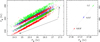 |
Fig. 6 Rotation Pψ and precession Pϕ periods of Apophis before and after the close encounter with Earth in April 2029 calculated from the purely gravitational model of the spin state change. Individual symbols come from 1000 nominal model simulations, with gravitational torques included, using statistically equivalent initial conditions on January 1, 2021. The three colors identify solutions starting from the three statistically equivalent initial solutions (compare with Fig. 1): red for the B-group, blue for the A-group, and green for the C-group. The right panel shows the current accuracy of the Apophis solution from the combination of the 2012-2013 and 2020–2021 observations. Those data are also reproduced in the left panel, but with a larger abscissa and ordinate scale, they are resolved only as single dots. The post-encounter Pϕ and Pψ values, spread over a large region, are shown on the left panel only. As expected, the uncertainty interval in both quantities expands by a factor larger than 103. The post-encounter median Pϕ value decreases to ≃25.75 h, while the median Pψ value remains about the same. |
4.2 Results
The initial rotation state and shape models of Apophis were constructed by bootstrapping observations from the 2012–2013 and 2020–2021 apparitions. We created 1000 such variants and set the epoch to January 1, 2021. These solutions were propagated using the model described in Sect. 4.1 with the final epoch in September 2029, well beyond the close approach to Earth in March 2029. We proceed in two steps. In Sect. 4.2.1 we first include only gravitational torques in the analysis. Next, in Sect. 4.2.2, we additionally demonstrate the potential role of the YORP torque.
4.2.1 Purely gravitational model
Figure 6 shows the predicted change in the two fundamental tumbling periods, namely the precession periods Pϕ at the abscissa and the rotation period Pψ on the ordinate. Similarly to the close encounter effect on the Apophis orbit, namely a huge stretch of the uncertainty interval in the osculating elements, the uncertainty in both periods significantly expands (by more than a factor 103). Still, the present fair constraint on their pre-encounter values makes the post-encounter uncertainty reasonably controlled. We find that the precession period will slightly decrease, while the rotation period ranges between ≃230 and ≃290 hours, roughly centered at the present value. There is also a clear correlation between Pϕ and Pψ demonstrated on the left panel of Fig. 6. These findings are similar but quite more accurate than those presented in Benson et al. (2023).
Figure 7 shows pre- and post-encounter values of the dimensionless parameter p = 2EB/L2, diagnostic about the tumbling mode. All values are smaller than unity, implying the post-encounter tumbling will remain in the SAM mode in this set of simulations. The right panel of this figure indicates that the mean effect of Earth’s gravitational torque during the encounter shifts the rotation state towards the separatrix between the SAM and LAM modes.
Finally, Fig. 8 shows the predicted change in orientation of the rotational angular momentum vector L in the inertial space. Prior to the effect displayed in this figure, which is entirely due to the Earth encounter, we note a steady (regular) precession due to the solar gravitational torque that amounts to about 3° in 8 years9. This effect has not been taken into account when fitting the available observations in Sect. 3, but this is justified by more than 10° uncertainty in the longitude of L. More than a 100° change in pole longitude during the Earth encounter appears dramatically large, but most of the effect is apparent. Due to near-polar latitude, the real tilt of L is much smaller. Its median value amounts to ≃9.8° only.
Taking into account the slight change in the orbital inclination, the median change in Apophis obliquity ϵ (defined here as the angle between the normal to the osculating orbit and the rotational angular momentum L) is only ≃5.7°. The fractional contribution to the change in the Yarkovsky acceleration is then estimated to ≃0.9%. This is formally larger than the current accuracy of the Yarkovsky effect determination for Apophis (about 0.5%; e.g., Farnocchia & Chesley 2022; Farnocchia et al. 2024). However, the post-encounter value of the Yarkovsky drift rate in semimajor axis da/dt is affected by more parameters than just the obliquity value. It turns out that the dominant contribution is due to the change in the semimajor axis, followed by a smaller contribution due to the rotation period. While detailed analysis should await until 2029, we note that the scaling da/dt ∝ a−1/2 cos ϵ made by Benson et al. (2023) is not correct. This is because it does not take into account the role of the thermal parameter Θ (see, e.g., Bottke et al. 2006; Vokrouhlický et al. 2015a). The slow rotation rate and high subsolar temperature imply Θ < 1, unless very high value of the surface thermal inertia Γ. For instance, assuming Γ ≃ 500 [SI units] (roughly at the upper limit of data reported in Müller et al. 2014; Satpathy et al. 2022; DellaGiustina et al. 2023), we have Θ ≃ 0.5. In this regime da/dt ∝ Θ, so an increase of Θ due to an increase of the semimajor axis and a slight decrease of the rotation period Pϕ will increase da/dt value. Considering the corresponding scaling ![Mathematical equation: $\[\mathrm{d} a / \mathrm{d} t \propto a P_{\phi}^{-1 / 2} ~\cos~ \epsilon\]$](/articles/aa/full_html/2026/05/aa58974-26/aa58974-26-eq30.png) , we may expect about 20% increase of the Yarkovsky effect from the analysis in this section (things might be modified if more significant changes in Pϕ and ϵ apply as in some simulations with the YORP torque discussed in the next section).
, we may expect about 20% increase of the Yarkovsky effect from the analysis in this section (things might be modified if more significant changes in Pϕ and ϵ apply as in some simulations with the YORP torque discussed in the next section).
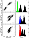 |
Fig. 7 Dimensionless parameter p = 2BE/L2 of Apophis’s spin. Left panel: pre-encounter values at the abscissa and the post-encounter values, calculated from the purely gravitational model of the spin state change, at the ordinate. As in the previous two figures, symbols come from 1000 nominal model simulations. Right panel: distribution of the p-values, pre-encounter in green, blue, and red for models C, A, and B, respectively, and post-encounter in black. As all values are smaller than unity, the rotation state remains in the SAM mode. The overall increase of the post-encounter values, however, implies the rotation stepped towards the separatrix of the SAM and LAM modes. |
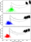 |
Fig. 8 Ecliptic longitude and latitude of the Apophis rotation angular momentum L before (green, blue, and red for models C, A, and B, respectively) and after (black) the close encounter to Earth in April 2029, calculated from the purely gravitational model of the spin state change. Individual symbols come from 1000 nominal model simulations, with gravitational torques included, using statistically equivalent initial conditions on January 1, 2021. All of the action, illustrated for our best-fit solution by the black line, occurs within ≃ ± 2 days centered at the Earth encounter. While the median longitude changes by more than 100°, the true tilt of L is far smaller because of the near-polar latitude. Its median value is ≃9.8°. Unlike the periods Pϕ and Pψ in Fig. 6, the post-encounter uncertainty region in longitude and latitude is not significantly stretched. |
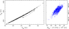 |
Fig. 9 Same as in Fig. 6 and model A, but now for a set of simulations including the YORP torque (8) with a fudge factor f = 0.4. Stretching of both Pϕ and Pψ periods is now larger by a factor of a few. |
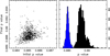 |
Fig. 10 Same as in Fig. 7 and model A, but now for a set of simulations including the YORP torque (8) with a fudge factor f = 0.4. The post-encounter p-values now exhibit a tail towards unity, which is a separatrix between SAM and LAM modes. |
4.2.2 Potential role of radiative torques
Next, we extend our simulations from the previous section by the effects of the YORP torque (8). Unlike the gravitational torques (7), which depend only on the dimensionless fractions α = B/A and β = B/C defined by the principal values of the inertia tensor, whose solution is part of the lightcurve inversion in Sect. 3, for the YORP torque, we have to define more parameters. We use the triangulated shapes from the lightcurve inversion for each of the 1000 bootstrapped variants of the solution A (having typically 900–1000 surface vertices). We assume uniform density of 2 g cm−3 and scale each of the models to a volume equivalent to a sphere of 400 m diameter, which is a rounded value of the diameter 417 m found by Brož et al. (2026) when scaling our Apophis shape model by occultations. For the sake of an illustration, we use a fudge factor f = 0.4 in (8). This value is a typical reduction by which the detected YORP values differ from the prediction of simple models like (8). We also ran simulations with smaller and larger values of f, but without observational constraints on the YORP effect for Apophis, we report their results only briefly. More efforts in this respect are postponed to further Apophis spin state models derived from more observational data (Sect. 5).
Figures 9–11 show again the change of the principal spin parameters by comparing their pre- and post-encounter values or distributions: (i) Pϕ and Pψ periods (Fig. 9), (ii) p parameter (Fig. 10), and (iii) direction of the rotational angular momentum vector L (Fig. 11). The p and L change is markedly larger than in Sect. 4.2.1, where only gravitational torques were considered, especially p values now have a tail towards unity (SAM to LAM separatrix limit). Nevertheless, in all tested variants of model A, the post-encounter tumbling state remained in the SAM mode for this value of the fudge factor (simulations with the fudge factor f ≥ 0.7 showed a small fraction of LAM post-encounter states, see also Benson et al. 2023). However, the main difference concerns the precession and rotation values. Their post-encounter values now exhibit a much larger spread.
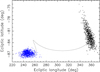 |
Fig. 11 Same as in Fig. 8 and model A, but now for a set of simulations including the YORP torque (8) with a fudge factor f = 0.4. The post-encounter pole latitude values now stretch beyond −80°. |
5 Conclusions
The photometric dataset of Apophis obtained during its two favorable apparitions in 2012–2013 and 2020–2021 is abundant, yet insufficient to uniquely determine the two periods of Apophis’s excited rotation. Due to the long interval between the apparitions not covered by the data, there are at least three different combinations of the precession and rotation periods that all produce about the same synthetic light curves and thus the same fit to the data. The possibility to constrain Apophis’s post-encounter state after April 2029, important among other topics for its future orbital evolution, including analysis of the Earth impact hazard (e.g., Vokrouhlický et al. 2015b), is the primary motivation for a unique and accurate pre-encounter model of its spin-state. This is because the resulting effect of Earth’s gravitational torque depends very sensitively on the exact phase of Apophis’s rotation state at the moment of the closest encounter.
In this work, we found that despite numerous and accurate past observations, neither uniqueness nor precision has yet been achieved. There are at least three statistically equivalent groups of solutions for Apophis’s spin state at this moment, and their prediction of its pre-encounter orientation is very similar, within 20° in terms of Euler angles. This is because the interval between the last apparition covered by the data and 2029 is eight years, which is the same interval as that between the observing windows in 2012–2013 and 2020–2021. Therefore, we can predict the approximate orientation of Apophis during its close encounter, but its accuracy is insufficient to reliably predict its post-encounter spin state so far. The simulations that include only the effect of Earth’s gravitational torques show that (i) the precession period will change from the current value of Pϕ = 27.374 ± 0.001 h towards shorter values between 24.5–27.5 h, and (ii) the rotation period will change from Pψ = 262.2 ± 0.1 h to the interval 230–290 h. At the same time, the direction of the rotational angular momentum vector will tilt by about 10°, and the rotation will stay in the SAM mode. When the so far unconstrained YORP torque is included in the model, the uncertainty of the prediction is much larger, with the post-encounter Pϕ ranging from 16 to 35 h and Pψ from 160 to 400 h.
Because the apparition in 2029 is not suitable for breaking the degeneracy in the rotation and precession periods, it is crucial to collect some photometric data before 2029. There will be an opportunity to take critical data to distinguish between the several possible models of Apophis’s spin state in 2027 and 2028. The observational conditions and requirements were discussed by Pravec & Ďurech (2024). Summarizing their findings briefly, we note that there will be observational windows for Apophis photometry from February to April 2027 and from December 2027 to June 2028 when Apophis will be >60° from Sun. The observing conditions will be particularly challenging in the February–April 2027 window when Apophis’s mean V is predicted to be 21.1–21.5 mag and large (4+m) telescopes in the northern hemisphere will be needed. The observing conditions will be slightly more favorable in the December 2027–June 2028 window, with Apophis’s mean V ranging from 19.2 to 20.7 mag; medium-sized (2–4m) telescopes in both hemispheres will be required. However, data taken in both observational windows may be needed not only to distinguish between the several possible Apophis’s spin models, but also to estimate or constrain the YORP effect in the asteroid. We encourage photometric observers to take the needed high-quality and extensive (though with a relatively low cadence) photometric data for Apophis in both apparitions.
Acknowledgements
This work was supported by the grant 23-04946S of the Czech Science Foundation. P.P. has been supported by the Praemium Academiae award (no. AP2401) from the Academy of Sciences of the Czech Republic. This publication uses data products from the TRAPPIST project funded by the Belgian National Fund for Scientific Research (F.R.S.-FNRS) under grant PDR T.0120.21. TRAPPISTNorth is funded by the University of Liege in collaboration with Cadi Ayyad University of Marrakech. Data were collected at the ESO La Silla Observatory. E.J. is the director of research at FNRS. Based on observations obtained with PESTO at the Mont-Mégantic Observatory, funded by the Université de Montréal, Université Laval, the Natural Sciences and Engineering Research Council of Canada (NSERC), the Fonds québécois de la recherche sur la Nature et les technologies (FQRNT), and the Canada Economic Development program. This paper was partially based on observations obtained at the Optical Wide-field Patrol Network (OWL-Net), the Sobaeksan Optical Astronomy Observatory (SOAO), the Lemmonsan Optical Astronomy Observatory (LOAO), the Bohyunsan Optical Astronomy Observatory (BOAO), and the Korea Microlensing Telescope Network (KMTNet), all of which are operated by the Korea Astronomy and Space Science Institute (KASI).
References
- Arai, T., & Destiny+ Team. 2025, in LPI Contrib., 3083, 2061 [Google Scholar]
- Ballouz, R. L., Agrusa, H., Barnouin, O. S., et al. 2024a, PSJ, 5, 251 [Google Scholar]
- Ballouz, R. L., Graninger, D. M., Adams, E. Y., et al. 2024b, LPI Contrib., 3006, 2060 [Google Scholar]
- Benson, C. J., Scheeres, D. J., Brozović, M., et al. 2023, Icarus, 390, 115324 [Google Scholar]
- Binzel, R. P., Rivkin, A. S., Thomas, C. A., et al. 2009, Icarus, 200, 480 [NASA ADS] [CrossRef] [Google Scholar]
- Bottke, Jr., W. F., Vokrouhlický, D., Rubincam, D. P., & Nesvorný, D. 2006, Ann. Rev. Earth Planet. Sci., 34, 157 [CrossRef] [Google Scholar]
- Breiter, S., Bartczak, P., Czekaj, M., Oczujda, B., & Vokrouhlický, D. 2009, A&A, 507, 1073 [NASA ADS] [CrossRef] [EDP Sciences] [Google Scholar]
- Breiter, S., Rożek, A., & Vokrouhlický, D. 2011, MNRAS, 417, 2478 [Google Scholar]
- Brož, M., Binzel, R. P., Vernazza, P., et al. 2026, A&A, 708, A162 [NASA ADS] [CrossRef] [EDP Sciences] [Google Scholar]
- Brozović, M., Benner, L. A. M., McMichael, J. G., et al. 2018, Icarus, 300, 115 [CrossRef] [Google Scholar]
- Brozovic, M., Benner, L. A. M., Naidu, S. P., et al. 2022, LPI Contrib., 2681, 2023 [Google Scholar]
- Čapek, D., & Vokrouhlický, D. 2004, Icarus, 172, 526 [Google Scholar]
- Cicalò, S., & Scheeres, D. J. 2010, Celest. Mech. Dyn. Astron., 106, 301 [Google Scholar]
- DellaGiustina, D. N., Nolan, M. C., Polit, A. T., et al. 2023, PSJ, 4, 198 [Google Scholar]
- DeMartini, J. V., Richardson, D. C., Barnouin, O. S., et al. 2019, Icarus, 328, 93 [NASA ADS] [CrossRef] [Google Scholar]
- Deprit, A., & Elipe, A. 1993, J. Astron. Sci., 41, 603 [Google Scholar]
- Dobrovolskis, A. R. 1996, Icarus, 124, 698 [NASA ADS] [CrossRef] [Google Scholar]
- Ďurech, J., Vokrouhlický, D., Pravec, P., et al. 2024, A&A, 682, A93 [NASA ADS] [CrossRef] [EDP Sciences] [Google Scholar]
- Farnocchia, D., & Chesley, S. R. 2022, LPI Contrib., 2681, 2007 [Google Scholar]
- Farnocchia, D., Chesley, S., Chodas, P., et al. 2013, Icarus, 224, 192 [Google Scholar]
- Farnocchia, D., Vokrouhlický, D., Čapek, D., Chesley, S. R., & DellaGiustina, D. N. 2024, LPI Contrib., 3006, 2046 [Google Scholar]
- Fatka, P., Pravec, P., Scheirich, P., et al. 2025, A&A, 695, A139 [NASA ADS] [CrossRef] [EDP Sciences] [Google Scholar]
- Fausnaugh, M. M., Burke, C. J., Caldwell, D. A., et al. 2021, TESS Data Release Notes:Sector 35, DR51, NASA Technical Memorandum, NASA/STI Accession number: 20210014771 [Google Scholar]
- Fitzpatrick, P. 1970, Principles of Celestial Mechanics (New York: Academic Press) [Google Scholar]
- Golubov, O., & Krugly, Y. N. 2012, ApJ, 752, L11 [NASA ADS] [CrossRef] [Google Scholar]
- Hapke, B. 1986, Icarus, 67, 264 [Google Scholar]
- Hapke, B. 2012, Theory of Reflectance and Emittance Spectroscopy (Cambridge: Cambridge University Press) [Google Scholar]
- Helfenstein, P., & Veverka, J. 1989, in Asteroids II, eds. R. P. Binzel, T. Gehrels, & M. S. Matthews (Tucson: University of Arizona Press), 557 [Google Scholar]
- Hirabayashi, M., Kim, Y., & Brozović, M. 2021, Icarus, 365, 114493 [NASA ADS] [CrossRef] [Google Scholar]
- Humes, O. A., & Hanuš, J. 2024, PSJ, 5, 271 [Google Scholar]
- Jehin, E., Gillon, M., Queloz, D., et al. 2011, The Messenger, 145, 2 [NASA ADS] [Google Scholar]
- Kaasalainen, M. 2001, A&A, 376, 302 [NASA ADS] [CrossRef] [EDP Sciences] [Google Scholar]
- Kaasalainen, M., & Torppa, J. 2001, Icarus, 153, 24 [NASA ADS] [CrossRef] [Google Scholar]
- Kim, Y., DeMartini, J. V., Richardson, D. C., & Hirabayashi, M. 2023, MNRAS, 520, 3405 [NASA ADS] [CrossRef] [Google Scholar]
- Landau, L., & Lifshitz, E. 1969, Mechanics (Oxford: Pergamon Press) [Google Scholar]
- Landolt, A. U. 1992, AJ, 104, 340 [Google Scholar]
- Lazzarin, M., Michel, P., Kueppers, M., et al. 2025, EPSC-DPS Joint Meeting, 2025, 806 [Google Scholar]
- Lee, H.-J., Ďurech, J., Vokrouhlický, D., et al. 2021, AJ, 161, 112 [NASA ADS] [CrossRef] [Google Scholar]
- Lee, H. J., Kim, M. J., Marciniak, A., et al. 2022, A&A, 661, L3 [NASA ADS] [CrossRef] [EDP Sciences] [Google Scholar]
- Li, J.-Y., Helfenstein, P., Burrati, B. J., Takir, D., & Clark, B. E. 2015, Asteroids IV, eds. P. Michel, F. E. DeMeo, & W. F. Bottke (Tucson: University of Arizona Press), 129 [Google Scholar]
- Licandro, J., Müller, T., Álvarez, C., Alí-Lagoa, V., & Delbo’, M. 2016, A&A, 585, 1 [Google Scholar]
- Lobanova, K. S., & Melnikov, A. V. 2024, Sol. Syst. Res., 58, 208 [Google Scholar]
- Michel, P., Lazzazin, M., Küppers, M., et al. 2025, LPI Contrib., 3083, 2012 [Google Scholar]
- Müller, T. G., Kiss, C., Scheirich, P., et al. 2014, A&A, 566, A22 [NASA ADS] [CrossRef] [EDP Sciences] [Google Scholar]
- Nolan, M. C., DellaGiustina, D. N., Polit, A. T., et al. 2025, EPSC-DPS Joint Meeting, 2025, 187 [Google Scholar]
- Pál, A., Szakáts, R., Kiss, C., et al. 2020, ApJS, 247, 26 [CrossRef] [Google Scholar]
- Polishook, D., & Aharonson, O. 2020, Icarus, 336, 113415 [Google Scholar]
- Pravec, P., & Ďurech, J. 2024, LPI Contrib., 3006, 2008 [Google Scholar]
- Pravec, P., Scheirich, P., Ďurech, J., et al. 2014, Icarus, 233, 48 [NASA ADS] [CrossRef] [Google Scholar]
- Reddy, V., Kelley, M. S., Dotson, J., et al. 2022, PSJ, 3, 123 [NASA ADS] [Google Scholar]
- Ricker, G. R., Winn, J. N., Vanderspek, R., et al. 2015, J. Astron. Teles. Instrum. Syst., 1, 014003 [Google Scholar]
- Rubincam, D. P. 2000, Icarus, 148, 2 [Google Scholar]
- Santana-Ros, T., Marciniak, A., & Bartczak, P. 2016, Minor Planet Bull., 43, 205 [NASA ADS] [Google Scholar]
- Satpathy, A., Mainzer, A., Masiero, J. R., et al. 2022, PSJ, 3, 124 [Google Scholar]
- Scheeres, D. J., Benner, L. A. M., Ostro, S. J., et al. 2005, Icarus, 178, 281 [Google Scholar]
- Scheeres, D. J., Abe, M., Yoshikawa, M., et al. 2007, Icarus, 188, 425 [NASA ADS] [CrossRef] [Google Scholar]
- Souchay, J., Lhotka, C., Heron, G., et al. 2018, A&A, 617, A74 [NASA ADS] [CrossRef] [EDP Sciences] [Google Scholar]
- Takahashi, Y., Busch, M. W., & Scheeres, D. J. 2013, AJ, 146, 95 [Google Scholar]
- Vokrouhlický, D., & Čapek, D. 2002, Icarus, 159, 449 [CrossRef] [Google Scholar]
- Vokrouhlický, D., Breiter, S., Nesvorný, D., & Bottke, W. F. 2007, Icarus, 191, 636 [Google Scholar]
- Vokrouhlický, D., Bottke, W. F., Chesley, S. R., Scheeres, D. J., & Statler, T. S. 2015a, in Asteroids IV, eds. P. Michel, F. E. DeMeo, & W. F. Bottke (Tucson: Tucson: University of Arizona Press), 509 [Google Scholar]
- Vokrouhlický, D., Farnocchia, D., Čapek, D., et al. 2015b, Icarus, 252, 277 [CrossRef] [Google Scholar]
- Whittaker, E. 1917, A Treatise on the Analytical Dynamics of Particles and Rigid Bodies (Cambridge: Cambridge University Press) [Google Scholar]
- Yu, Y., Richardson, D. C., Michel, P., Schwartz, S. R., & Ballouz, R.-L. 2014, Icarus, 242, 82 [Google Scholar]
- Zola, S., Kouprianov, V., Reichart, D. E., Bhatta, G., & Caton, D. B. 2021, Rev. Mex. Astron. Astrofis. Conf. Ser., 53, 206 [Google Scholar]
- Zola, S., Stachowski, G., Kurowski, S., et al. 2025, Rev. Mex. Astron. Astrofis. Conf. Ser., 59, 31 [Google Scholar]
In practice, our code works with the parameter S(0) = B0w(1 − g)/(1 + g)2 defined by Hapke (1986), which is for w = 0.23, g = −0.27 equal to S(0) = 0.88, which was the value that we fixed.
As Figure 5 shows Apophis will approach the Moon about 16 hours after the closest encounter with Earth. However, we do not include this body in our simulation at this moment. Not only is the lunar mass nearly two orders of magnitude smaller than that of Earth, but also the closest distance to the Moon will be about 2.5 times larger than to Earth. As a result, the maximum of the lunar torque on Apophis spin will be ≃1300 times smaller.
The times of the closest approach differed by 0.5 s; the distances at the closest approach by 1 km.
This value is well expected and roughly corresponds to the pole precession of (2100) Ra-Shalom on a similar heliocentric orbit and having a similarly slow rotation (see Ďurech et al. 2024).
Appendix A Aspect data
Aspect data for new observations from 2020–2021 taken with the Danish telescope, ESO, La Silla.
Aspect data for new observations from 2020–2021.
Appendix B Light curve fit
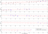 |
Fig. B.1 Fit of the model to the photometric data from 2012–2013. The red curve is the synthetic light curve produced by model A*. The points are photometric measurements published by Pravec et al. (2014). The blue color marks the accurately calibrated subset observed with the Danish telescope, which was used to reconstruct model A. Some of the grey light curves, which were taken with other telescopes, are shifted with respect to the model due to their imperfect photometric calibrations. The vertical axis is the Cousins R reduced to the unit distances from Earth and Sun. |
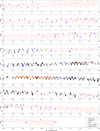 |
Fig. B.2 Fit of the model to the photometric data from 2020–2021. The red curve is the synthetic light curve produced by model A*. The points are photometric measurements from various sources (see the legend and Table A.2). The blue points represent absolutely calibrated photometry from the Danish telescope that was used to reconstruct model A. The vertical axis is the Cousins R reduced to the unit distances from Earth and Sun. |
All Tables
Aspect data for new observations from 2020–2021 taken with the Danish telescope, ESO, La Silla.
All Figures
|
Fig. 1 Period scan. The plots show the residuals (blue points) of the fit for different values of the precession period Pϕ (left) and the rotation period Pψ (right). The dotted vertical lines indicate the positions of the eight best solutions, and the red crosses represent RMS residuals for the high-resolution models. The distances between local minima ΔPϕ and ΔPψ are denoted. |
| In the text | |
|
Fig. 2 Period scan. The plot shows the same data as in Fig. 1, but here the RMS residuals are color coded, and both the precession period Pϕ and rotation period Pψ are plotted to visualize the correlation between them. The best solutions with the lowest residuals (blue color) lie on the red dashed line that is in fact part of a hyperbola satisfying the relation |
| In the text | |
|
Fig. 3 Evolution of Euler angles for models A (blue), B (red), and C (green). The plots show the evolution of Euler angles ϕ, θ, and ψ within a month in different years. All three angles are similar for all three models in the years 2013, 2021, and 2029 because they are separated by 8 years. The Euler angles, and thus the orientation of the models, differ for epochs between these years (e.g., March 2027). |
| In the text | |
|
Fig. 4 Best models A (top) and A* (bottom) with parameters listed in Table 2. Model A was constructed from a subset of accurately calibrated photometry from the Danish telescope (La Silla) and TESS observations, while for model A*, we used all available photometry. |
| In the text | |
|
Fig. 5 Parameters of the Apophis close encounter with Earth on April 13, 2029. The top panel shows the geocentric (solid line) and selenocentric (dashed line) distance, and the bottom panel shows the relative geocentric and selenocentric velocity. The origin of the abscissa is at the nominal Earth closest approach epoch 62239.90709 (MJD). The horizontal dashed line at the top panel indicates the closest approach distance of 38 012 km, the horizontal dashed lines at the bottom panel show the relative geocentric velocities at the closest approach, 7.42 km s−1, and the asymptotic value, 5.84 km s−1. The closest approach to the Moon is at 95 959 km. The black arrow shows the Apophis Pϕ timescale for reference. |
| In the text | |
|
Fig. 6 Rotation Pψ and precession Pϕ periods of Apophis before and after the close encounter with Earth in April 2029 calculated from the purely gravitational model of the spin state change. Individual symbols come from 1000 nominal model simulations, with gravitational torques included, using statistically equivalent initial conditions on January 1, 2021. The three colors identify solutions starting from the three statistically equivalent initial solutions (compare with Fig. 1): red for the B-group, blue for the A-group, and green for the C-group. The right panel shows the current accuracy of the Apophis solution from the combination of the 2012-2013 and 2020–2021 observations. Those data are also reproduced in the left panel, but with a larger abscissa and ordinate scale, they are resolved only as single dots. The post-encounter Pϕ and Pψ values, spread over a large region, are shown on the left panel only. As expected, the uncertainty interval in both quantities expands by a factor larger than 103. The post-encounter median Pϕ value decreases to ≃25.75 h, while the median Pψ value remains about the same. |
| In the text | |
|
Fig. 7 Dimensionless parameter p = 2BE/L2 of Apophis’s spin. Left panel: pre-encounter values at the abscissa and the post-encounter values, calculated from the purely gravitational model of the spin state change, at the ordinate. As in the previous two figures, symbols come from 1000 nominal model simulations. Right panel: distribution of the p-values, pre-encounter in green, blue, and red for models C, A, and B, respectively, and post-encounter in black. As all values are smaller than unity, the rotation state remains in the SAM mode. The overall increase of the post-encounter values, however, implies the rotation stepped towards the separatrix of the SAM and LAM modes. |
| In the text | |
|
Fig. 8 Ecliptic longitude and latitude of the Apophis rotation angular momentum L before (green, blue, and red for models C, A, and B, respectively) and after (black) the close encounter to Earth in April 2029, calculated from the purely gravitational model of the spin state change. Individual symbols come from 1000 nominal model simulations, with gravitational torques included, using statistically equivalent initial conditions on January 1, 2021. All of the action, illustrated for our best-fit solution by the black line, occurs within ≃ ± 2 days centered at the Earth encounter. While the median longitude changes by more than 100°, the true tilt of L is far smaller because of the near-polar latitude. Its median value is ≃9.8°. Unlike the periods Pϕ and Pψ in Fig. 6, the post-encounter uncertainty region in longitude and latitude is not significantly stretched. |
| In the text | |
|
Fig. 9 Same as in Fig. 6 and model A, but now for a set of simulations including the YORP torque (8) with a fudge factor f = 0.4. Stretching of both Pϕ and Pψ periods is now larger by a factor of a few. |
| In the text | |
|
Fig. 10 Same as in Fig. 7 and model A, but now for a set of simulations including the YORP torque (8) with a fudge factor f = 0.4. The post-encounter p-values now exhibit a tail towards unity, which is a separatrix between SAM and LAM modes. |
| In the text | |
|
Fig. 11 Same as in Fig. 8 and model A, but now for a set of simulations including the YORP torque (8) with a fudge factor f = 0.4. The post-encounter pole latitude values now stretch beyond −80°. |
| In the text | |
|
Fig. B.1 Fit of the model to the photometric data from 2012–2013. The red curve is the synthetic light curve produced by model A*. The points are photometric measurements published by Pravec et al. (2014). The blue color marks the accurately calibrated subset observed with the Danish telescope, which was used to reconstruct model A. Some of the grey light curves, which were taken with other telescopes, are shifted with respect to the model due to their imperfect photometric calibrations. The vertical axis is the Cousins R reduced to the unit distances from Earth and Sun. |
| In the text | |
|
Fig. B.2 Fit of the model to the photometric data from 2020–2021. The red curve is the synthetic light curve produced by model A*. The points are photometric measurements from various sources (see the legend and Table A.2). The blue points represent absolutely calibrated photometry from the Danish telescope that was used to reconstruct model A. The vertical axis is the Cousins R reduced to the unit distances from Earth and Sun. |
| In the text | |
Current usage metrics show cumulative count of Article Views (full-text article views including HTML views, PDF and ePub downloads, according to the available data) and Abstracts Views on Vision4Press platform.
Data correspond to usage on the plateform after 2015. The current usage metrics is available 48-96 hours after online publication and is updated daily on week days.
Initial download of the metrics may take a while.