| Issue |
A&A
Volume 709, May 2026
|
|
|---|---|---|
| Article Number | A13 | |
| Number of page(s) | 21 | |
| Section | Stellar structure and evolution | |
| DOI | https://doi.org/10.1051/0004-6361/202558585 | |
| Published online | 08 May 2026 | |
JOYS: Unlocking accretion-rate diagnostics for high-mass protostars using JWST/MIRI HI lines
1
Max-Planck-Institut für Astronomie, Königstuhl 17, D-69117 Heidelberg, Germany
2
Leiden Observatory, Leiden University, PO Box 9513, 2300 RA, Leiden, The Netherlands
3
Max Planck Institut für Extraterrestrische Physik (MPE), Giessen-bachstrasse 1, 85748 Garching, Germany
4
INAF–Osservatorio Astronomico di Capodimonte, Salita Moiariello 16, 80131 Napoli, Italy
5
Department of Physics, Maynooth University, Maynooth, Co. Kildare, Ireland
6
UK Astronomy Technology Centre, Royal Observatory Edinburgh, Blackford Hill, Edinburgh EH9 3HJ, UK
7
Department of Space, Earth and Environment, Chalmers University of Technology, Onsala Space Observatory, 439 92 Onsala, Sweden
8
Space Science and Astrobiology Division, NASA’s Ames Research Center, Moffett Field, CA 94035, USA
9
Institut de Ciencies de l’Espai (ICE-CSIC), Campus UAB, Carrer de Can Magrans S/N, 08193 Cerdanyola del Valles, Catalonia, Spain
10
Institut d’Estudis Espacials de Catalunya (IEEC), c/ Gran Capitá, 2–4, 08034 Barcelona, Spain
11
School of Cosmic Physics, Dublin Institute for Advanced Studies, 31 Fitzwilliam Place, D02 XF86 Dublin, Ireland
12
INAF-Osservatorio Astronomico di Roma, Via di Frascati 33, 00078 Monte Porzio Catone, Italy
13
Laboratory for Astrophysics, Leiden Observatory, Leiden University, PO Box 9513, 2300 RA, Leiden, The Netherlands
★ Corresponding author: This email address is being protected from spambots. You need JavaScript enabled to view it.
Received:
15
December
2025
Accepted:
15
March
2026
Abstract
Context. While many aspects of high-mass star formation have been investigated, the accretion onto the central protostars is one of the most fundamental but less explored physical properties. The James Webb Space Telescope (JWST), through its Mid InfraRed Instrument (MIRI), offers a unique opportunity to explore tracers of accretion at less-extincted wavelengths (5–27 μm) than those studied so far, where it delivers unparalleled sensitivity and spectral resolution.
Aims. We probed the capability of MIRI in its MRS/IFU mode to detect and resolve atomic Hydrogen (H I) emission lines in such embedded objects to subsequently estimate accretion luminosities (Lacc) and accretion rates (Ṁacc) for the first time in a sample of (six) high-mass, star forming regions at different evolutionary stages.
Methods. We used the dereddened H I line luminosities as tracers of accretion by applying line-to-accretion-luminosity relations (Lacc-calibrations) from the literature. As such Lacc-calibrations were originally established for low-mass Class II objects, we assessed their applicability to our sample prior to estimating accretion rates. Extinction was derived from the silicate absorption feature at 9.7 μm.
Results. The infrared continuum reveals, at much higher spatial resolution than before, the location of new infrared sources (protostars), towards which we detected a handful of H I lines. While a few lines are secure detections, many are tentative. The most commonly detected line is Humphreys α at 12.37 μm, followed by Humphreys β and Pfund α. Assuming that their line fluxes are dominated by accretion, we find that two of the three existing Lacc-calibrations predict excessively high accretion luminosities that largely exceed their bolometric luminosities (Lbol), and that the third Lacc-calibration still overpredicts accretion luminosities for some sources. Considering the given uncertainties, estimated accretion rates are only tentative.
Conclusions. This work demonstrates the great potential of JWST/MIRI to probe H I line emission that originated in the innermost regions of high-mass protostellar systems, setting the ground floor for further investigations into accretion in these objects. While this project had the ambitious goal of robustly quantifying accretion rates, we shed light on what outstanding methodological challenges remain; the most critical being the development of new Lacc- calibrations for intermediate- to high-mass protostars.
Key words: accretion / accretion disks / stars: formation / stars: massive / stars: protostars / stars: winds / outflows
© The Authors 2026
 Open Access article, published by EDP Sciences, under the terms of the Creative Commons Attribution License (https://creativecommons.org/licenses/by/4.0), which permits unrestricted use, distribution, and reproduction in any medium, provided the original work is properly cited.
This article is published in open access under the Subscribe to Open model.
Open access funding provided by Max Planck Society.
1. Introduction
The processes governing the accretion of material from the inner protoplanetary disk onto the central star likely vary across mass regimes. While they are well known for low-mass, pre-main-sequence (PMS) stars with discs, much less is known about the intermediate- and high-mass sources. Furthermore, accretion during the deeply embedded phases (first ∼105 years for low-mass protostars; Dunham et al. 2015), where the central star and disc are obscured by the dusty envelope, is poorly understood; yet, it is the time when stars gain the majority of their final masses (see review of Hartmann et al. 2016 for masses below 5 M⊙ and Beuther et al. 2025 for a comprehensive review of both the low- and high-mass regimes).
For low-mass PMS stars with discs –that is, T-Tauri Stars (TTS)– the general picture is clearer as their dissipated envelope no longer obscures the optical or infrared (IR) light coming from its central source. At this phase, the disc is truncated by the magnetic field produced by the star, while the star’s radiation sublimates the inner disc dust within a dust destruction radius. As a consequence, flows of material fall at free-fall speeds onto the star due to gravity, following the magnetic-field lines (Koenigl 1991); at the same time, another fraction can be ejected as magnetohydrodynamical (MHD) or photoevaporative winds and jets. The inflows of material are episodic and in the form of column or funnel flows that reach temperatures of about 104 K. Near the stellar chromosphere a shock is produced, converting kinetic energy into radiation (Bhandare et al. 2025) and briefly raising temperatures up to ∼106 K (Hartmann et al. 2016). This radiation can be seen as a continuum excess that peaks in the UV (Koenigl 1991) but can also be observed at the optical and near-infrared (NIR). The gas along the accretion funnels is excited and shows H I lines emitting at optical (e.g. H α, H β lines; Hamann & Persson 1992; Bouvier et al. 2007), NIR (e.g. Paα, Paβ, Brα), and mid-infrared (MIR; e.g. Hu α; Beuther et al. 2023) wavelengths, both from the shock and funnel flows (and potentially winds). Due to their larger surface area, funnel flows may dominate the bulk of the observed line emission.
For the high-mass regime (M≥ 8 M⊙) it still remains unknown whether the same (magnetospheric) processes hold. Massive sources may no longer accrete through funnel flows because they are thought to become rather radiative instead of convective as they grow in mass (Stahler & Palla 2004), meaning that their magnetic field should no longer dominate the physics of accretion. It is also unclear whether the H I emission in these objects is only tracing accretion or might be dominated by circumstellar ionised gas.
An alternative theory of disk evolution (derived for low-mass TTSs) that may explain the accretion onto massive stars is the boundary layer scenario presented in Lynden-Bell & Pringle (1974). In the case where magnetic fields are not dominant, the disc extends towards the stellar photosphere (filling the gap produced in the magnetospheric process) and grazes the relatively steady stellar atmosphere, meaning that the material enters the star while angular momentum is dissipated outwards. Here, emission would arise from viscous dissipation that converts part of the gravitational energy into continuum luminosity that peaks in the UV, similarly to the magnetospheric shocks, while the variability might be explained by the suddenness of the entry of orbital material into the stellar atmosphere (Lynden-Bell & Pringle 1974).
To produce emission lines, the hydrogen electrons must be excited to higher quantum levels by a certain energy source such that they can spontaneously de-excite or recombine to lower levels. A couple of models exist in the literature that explain what processes drive this energy input. Case B recombination (Baker & Menzel 1938) was initially proposed to explain the Balmer decrement on Nebulae under the hypothesis that it is opaque to the Lyman series, but it has been also invoked to explain the H I emission lines seen in Classical T-Tauri Stars (CTTSs), in which case the inflowing plasma is photoionised, producing free electrons that can subsequently recombine. Under this assumption, the accreting flows would produce broad emission lines of atoms and molecules, while the region of the shock would generate relatively narrow lines (Hartmann et al. 2016). Until the growing central star has not yet reached 8 M⊙, shock UV radiation might be responsible for heating up the funnel flows until ionisation occurs. If not radiation, an unknown magnetic mechanism may apply (Hartmann et al. 2016). Case-B emissivities were studied in Hummer & Storey (1987) while testing collisional excitation effects up to quantum level n = 3. The authors found that if collisions from the ground states to level three are significant, derived Case-B emissivity ratios are no longer valid because contamination of other upper levels is also implied.
More recently, alternative emissivity-ratio models of Kwan & Fischer (2011) (KF11) studying the local conditions of the flowing material (either accretion flows or winds), suggested that collisional excitation (CE) is the primary mechanism responsible for the H I-line production. Here, collisions are powered by the intrinsic thermal kinetic energy of the flow itself, relegating recombination due to irradiation (Case B) to a less significant role. Collisional excitation points to flow temperatures between 8750 and 1.25 × 10⁴ K and to H I-line emissivities that strongly depend on volume densities and temperature. Both Case B and CE suggest specific hydrogen-line ratios under different temperature, electron density (Case B), volume density (CE), or ionisation rate (CE) conditions, which can be used to infer the properties of the gas producing the lines depending on the adopted model. In this regard, the H I-line ratios observed by Edwards et al. (2013) for a sample of 16 TTSs give support to the local conditions scenario where collisions are protagonists. Given all of these, not a single theory has yet been derived to explain line emission in the environments of high-mass (≥8 M⊙) protostars. This makes sense because high-mass sources are much harder to probe since they transition directly from the protostellar phase to the main sequence (Palla & Stahler 1999) without offering an exposed disc that it is still accreting material (pre-main-sequence phase).
The most direct approach to measure accretion luminosity (Lacc) is obtained from excess emission above the photosphere continuum, most commonly in the UV but also in the optical or IR (Gullbring et al. 2000; Donehew & Brittain 2011), and it can be studied simultaneously with H I lines in PMS stars to search for scaling relations that allow us to estimate accretion luminosities (i.e. a calibration) when direct methods are no longer possible, for example due to high extinction in the line of sight (LOS). In this regard, works focused on NIR lines such as Pa β, Br γ, and Pf β (Grant et al. 2022; Muzerolle et al. 1998; Alcalá et al. 2014; Salyk et al. 2013) have found such correlations, confirming that the strength of H I lines can be used as tracer of Lacc. In protostellar systems, extinctions are usually high enough to make NIR lines undetectable, and thus the search for such tracers has shifted towards even longer wavelengths.
In the MIR regime, Rigliaco et al. (2015) found a correlation between the intensity of the Humphreys α line (denoted Hu α or H I 7−6) at 12.372 μm for PMS stars with the luminosity of the Hα line in the optical (calibrated in Rigliaco et al. 2012) using the Spitzer Space Telescope. This demonstrates that other H I lines can similarly be used as tracers of the accretion luminosity. It has recently become possible to establish new MIR H I lines as Lacc tracers with the JWST (Tofflemire et al. 2025 and Shridharan et al. 2026), adding a total of seven H I lines (in the 5.9−19 μm range) to the set of available tracers, which we can, in principle, use to study accretion rates in embedded objects (see Table 4).
For low-mass Class II objects, the NIR H I tracers yield Ṁacc ≲ 10−8 M⊙ yr−1 (Alcalá et al. 2014), while for the intermediate-mass regime they point to Ṁacc between ∼10−8 and 10−4 M⊙ yr−1 (Grant et al. 2022; Wichittanakom et al. 2020; Rogers et al. 2025), although sometimes with a large dispersion. For the high-mass side, we can refer to theoretical works, which suggest higher Ṁacc up to ∼ 10−4 M⊙ yr−1 set by their periodic accretion outbursts, which should progressively decrease as the star evolves to the main-sequence phase (Hartmann 2008). As the embedded phases are hard to probe, most of the observational constraints come from their corresponding outflow ejection rates, because they are thought to represent a fraction (∼1%) of the accretion rates (Shepherd & Churchwell 1996a,b; Beuther et al. 2002b; Arce et al. 2007; Frank et al. 2014).
Given the newly available high sensitivity of the JWST, the Hu α line becomes suitable for observations of embedded objects. In this line, Beuther et al. (2023) reported a tentative three-sigma detection of Hu α in the high-mass binary IRAS23385. Building on this initial study, we performed a more exhaustive search; the goal was to disentangle the accretion occurring at the very early stages of high-mass star formation for the first time. Our sample consists of six high-mass star forming environments, which can be classified as infrared dark clouds (IRDCs), high-mass protostellar objects (HMPO), and hot molecular cores (HMC). Each of these regions is expected to host embedded stars with masses above − or in the process of reaching − 8 M⊙.
To measure accretion rates, we studied H I-accretion tracers available within the MIRI/JWST spectral coverage, assuming that the accretion luminosity relationships can be extended from Class II, low-mass YSOs to high-mass protostars (however, see discussion). We present the JWST data in Sect. 2, and describe our methods in Sect. 3. We show all the H I lines that MIRI detected towards our regions, and present our results on accretion luminosities and rates in Sect. 4. We elaborate on relevant methodological uncertainties and limitations that can affect the accuracy of accretion luminosity (and rate) measurements in Sect. 5, and we provide our conclusions in Sect. 6.
2. Data
This release is part of the MIRI GTO JWST Observations of Young proto-Stars (JOYS) programme, which observed more than 20 star forming regions with the Medium Resolution Spectrometer (MRS), including six high-mass regions (PID 1290; PI: E. F. van Dishoeck). This work focused specifically on their sub-sample of high-mass sources, which can be classified as two stages of evolution: the more active and hence evolved IRAS23385, G31, and IRAS18089; and the comparatively more quiescent, younger G28IRS2, G28P1, and G28S. Figures 1 and 2 give an overview of our sample, where beam sizes are 0.3 and 0.6 arcseconds at 5 and 14 μm, respectively. The spectral resolving power ranges between 3500 and 3000 at 5 and 14 μm, respectively, and the typical noise level is ∼2 × 10⁻⁵ Jy at the IR source locations.
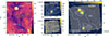 |
Fig. 1. Overview of three less evolved regions of our sample: G28IRS2, G28P1, and G28S. In this case, all of them belong to the same IRDC G28. Left: Spitzer (8 μm) view of the whole IRDC G28. The three target sub-regions are depicted with millimetre contours (white) from ALMA for G28IRS2 (Molinari et al. 2025) and G28P1 (Zhang et al. 2015), and from SMA for G28S (Feng et al. 2016a), with cyan boxes highlighting the field of view of our MIRI observations, which are slightly magnified for better visualisation. Middle and right panels: Zoomed-in views of the target sub-regions. These show the MIRI continuum at 14 μm, whereas cyan contours trace the continuum at 5 μm (no IR source was detected towards G28S). The ellipses in the bottom right corners represent beam sizes: grey for the 14 μm image and cyan for the 5 μm contours. |
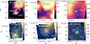 |
Fig. 2. Overview of three more evolved protostellar regions of our sample: IRAS18089, G31, and IRAS23385. Top panels: Each region as seen by Spitzer (3.6 μm) or WISE (12 μm), with white contours depicting millimetre data from ALMA for IRAS18089 (1.2 mm; Sanhueza et al. 2021) and G31 (1.3 mm; Beltrán et al. 2018), or NOEMA for IRAS23385 (1 mm; Beuther et al. 2018). The cyan boxes highlight the field of view of our MIRI observations. Bottom panels: MIRI integrated images at 14 μm for each region covering the corresponding upper panels. The cyan contours represent the continuum at 5 μm. |
2.1. Ancillary data
Previous observations at millimetre wavelengths (from 1 to 1.3 mm) provide general properties of our target regions (Table 1 and references therein). In particular, we retrieved archival data from ALMA for IRAS18089 (Sanhueza et al. 2021), G31 (Beltrán et al. 2018), G28IRS2 (Molinari et al. 2025), and G28P1 (Zhang et al. 2015); NOEMA for IRAS23385 (Beuther et al. 2018); and SMA for G28S (Feng et al. 2016a).
JOYS source sample from millimetre observations.
3. Methods
3.1. Data reduction
We ran our JOYS-adapted version of the MIRI JWST pipeline (version 1.15.1), in line with all JOYS releases. Steps are detailed in van Gelder et al. (2024b,a), but as we ran an updated JWST pipeline version there are a few differences that we mention here. We included background subtraction on the detector level when available, namely for IRAS18089 and G31. In these cases, we masked science emission lines (i.e. H2 0-0 S(1), H2 0-0 S(2), and [Ne II]) on the background files prior to reduction. Despite it also being available for IRAS23385, we did not implement it because it contains significant emission of several species. Although planned originally, background observations for G28IRS2, G28P1, and G28S were not taken. In all cases, the residual fringe correction and bad pixel correction tasks were turned on. The outlier pixel detection task was turned off. We note, however, that bad pixels are commonly seen, and they represent an obstacle that cannot be fully overlooked. Some can be seen in Fig. 4 (G28P1 A) as a repeated pattern of pixels spread out on the map. In our case, they are harmless, as they appear out of our science apertures. Lastly, for IRAS23385 in particular, we masked cosmic rays in the science files that appeared at the wavelengths of some hydrogen emission lines.
3.2. Astrometric correction
We used MIRI parallel images at 15.0 μm, their associated MIRI point source catalogues, and Gaia DR3 to identify and correct pointing deviations of the JWST relative to Gaia. We found matching sources between MIRI and Gaia for three regions (G28IRS2, G28S, and G31), which revealed a small systematic shift of the JWST pointing of ∼124 mas in right ascension and 30 mas in declination on average. Such an average shift is in fact comparable to the angular resolution of the JWST at 5 μm (130 mas). We corrected our MIRI astrometry using the individual values found for each source, and for the remaining three regions we adopted different approaches, which we describe in detail in Appendix B.1.
3.3. Continuum subtraction
To study line features, we performed a pixel-wise subtraction of the continuum around each line. To do so, we first masked a small spectral range at the science lines; then, we obtained the best fit among polynomial functions of the order of one, two, and three using a root-mean-squared error (RMSE) criterion. The selected function was finally subtracted from the corresponding original pixel spectrum. The second- and third-order polynomials were only strictly necessary for IRAS18089 (Appendix B.2), and relevant for the bright G31 outflow, but we still included them for the other regions for consistency and because they still offer slightly better continuum fits.
As described, the procedure achieved clean line maps for five out of our six regions, but for IRAS18089 a few more considerations were necessary. We provide details for IRAS18089 in Appendix B.2. Although the subtraction procedure could not be applied equally to all regions, we emphasise that we achieved data cubes with homogeneous spectral noise across the entire sample (up to 10−4 Jy).
3.4. Searching for accretion tracers: Strategy
H I emission lines contain key information about the accretion processes occurring in a protostar. We searched for all the hydrogen lines that can be detected given the sensitivity of our MIRI/MRS observations (from 5 to 28 μm). To achieve this, we tested the 25 H I lines in that wavelength range that involve a maximum of five quantum level transitions of the electron, namely Δn = nu − nl ≤ 5. We introduce them in Table A.1 where they are organised by increasing wavelength. Transitions involving larger values of Δn are most likely not detectable given our sensitivity. To also account for line contaminants, we tested the presence of water line emission as they are often found towards Class II sources (Rigliaco et al. 2015).
We used a typical radius of  to set the protostar apertures when extracting their spectra, both for estimating extinctions (Sect. 3.5) and studying emission lines (Sect. 4.3). Simultaneously, we evaluated their local background as an annulus centred on the protostar with a typical radius of
  (excluding the protostar’s aperture); although in some cases, to correctly represent the local ambient conditions, we arbitrarily shifted it from the protostar position or varied their angular sizes (between
  and
and  ). This was done to avoid the noisier image edges (e.g. G28P1 in Fig. 4) or areas affected by strong ionisation driven by external sources (e.g. IRAS23385 or IRAS18089 in Figures A.2 and A.4, respectively). We computed the signal-to-noise ratio (S/N) as the line emission peak over the baseline uncertainty, and additionally introduced a protostar-to-background line luminosity (Lproto/Lbkg) ratio (Table 5) to properly assess the significance of compact detections towards the protostars. We only classified an H I line as a ‘compact detection’ when S/N ≥3 and Lproto/Lbkg > 1.
3.5. Extinction Aλ
We estimated extinction at a given wavelength, Aλ, in two steps: we first obtained AK for each protostar from the absorption depth of the silicate feature (τ9.7) and then converted AK to the wavelength of interest, Aλ (H I lines), using the two extinction curves of Pontoppidan et al. (2024) and McClure (2009). We hereafter refer to them as the KP5 and M09 extinction curves, respectively. Our specific approach follows that of Gieser et al. (2026), which builds on the analysis of Rocha et al. (2024). For a summary of ways to measure extinction, see van Dishoeck et al. (2025, Appendix G).
In step one, we used the same sky aperture used to study the protostellar spectra (Sect. 3.4). The main absorption feature of silicates at 9.7 μm is mainly produced by silicate grains along the line of sight towards the central source, and its depth is what we aim to measure. We modelled silicate dust compositions as mixtures of olivine and pyroxene following the synthetic silicate models of Rocha et al. (2024). As the bending mode (secondary) feature of silicates at ∼18 μm is mixed with water ice absorption, we included water ice models at temperatures of 15 and 75 K following Gieser et al. (2026). These two are the only absorbing species that we modelled. In parallel, we modelled the emitting source as that of two blackbody components representing warm emission due to the embedded protostar and cold emission due to the dusty protostellar envelope. Only for G28IRS did we require the addition of a third (hot) blackbody component. Lastly, we provided the fitter with spectra masked to include only the four spectral ranges indicated in Fig. 3 (R1–R4), because at those wavelengths the water and silicate absorption should dominate over that of other species. These input spectra were also re-binned by a factor of five to smooth out noisy ranges or strong emission lines. In more detail, range R1 is defined as where we expect minimal absorption features; thus, it provides the closest look at the global IR continuum. Range R2 represents the short-wavelength slope of the main silicate feature, which is expected to be dominated by silicates, extending towards the feature peak but before reaching the noise level. R3 is defined as where H2O (libration) absorption becomes dominant over the silicates up to the prominent CO2 absorption feature at ∼15 μm, and avoiding the broad PAH emission feature (at 11.28 μm) when present. This also means that these ranges are adapted for each region independently. Lastly, R4 marks the secondary silicate feature that still has some H2O libration absorption.
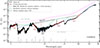 |
Fig. 3. Full MIRI spectrum of the G28IRS2 protostar (black). It shows several absorption features, where the broader one at 9.7 μm is produced by silicate grains. Blackbody components (3 in this case) absorbed by silicates and H2O were fitted to reproduce the overall continuum. The blue curve represents the fit obtained by considering spectral ranges that are predominantly absorbed by silicates and H2O (in red, also indicated by the R1–R4 ranges). The green curve represents blackbody emission that would only be absorbed by silicates, while the dotted magenta curve shows the modelled blackbody emission unaffected by absorption. The dashed black curve above the main silicate absorption feature at 9.7 μm is an interpolation of the silicate-absorbed continuum from a five-order polynomial fit. Here, the vertical red line highlights the resulting depth of the feature that determines τ9.7, whose uncertainty is given by another two polynomials (of the order of 1 and 4) fits passing above and below (grey curves). The dashed black line at R4 indicates the location of the secondary silicate absorption feature. |
Given this setup, the fitter used non-linear least squares to optimise a total of eight parameters: two blackbody temperatures with their corresponding scaling factors that represent their emitting surface sizes (3 blackbodies for G28IRS2); abundances of olivine and pyroxene; and abundances of H2O at two temperatures (15 and 75 K; Table A.2). In Sect. 4.2, we discuss the structure and properties of these protostellar systems as derived from the models. For a better representation of the noisy ranges between 8.8 and 11 μm or between 5.8 and 7.4 μm, some sources’ spectra were binned by factors of four (IRAS18089C), five (G28P1 A and B) or ten (G28IRS2).
To obtain the depth of the main silicate feature at λ ∼ 9.7 μm (τ9.7), we estimated its baseline through polynomial fits connecting the resulting silicate absorbed spectrum (green curve in, e.g. Fig. 3) from 7 to 14 μm but masked at the silicate feature between 7.6 and 12.4 μm. Depending on the source, the selected polynomial is of the third, fourth, or fifth order, and it is always represented as a black curve (Figures 3, A.6, and A.7). The depth of the silicate feature τ9.7 is illustrated with a vertical dashed line, and we calculated it using
 (1)
(1)
where  is the baseline flux passing above this absorption feature (as just described), and
  is the flux at its minimum. We note here that in several cases this fitted minimum appears below the noise floor, which occurs because the noise floor is hiding the tip of the main silicate feature in all our sources. When the fit does not go deeper than the noise floor, one might consider its derived τ9.7 as a lower limit (possibly IRAS18089 A and C). To estimate the uncertainty on τ9.7, we adopted other two polynomial fits (of the order of 2, 3, 4, or 5) that fit different baselines passing above and below the selected one, resulting in an asymmetric uncertainty for τ9.7. They are also displayed in Figures 3, A.6, and A.7. We subsequently converted τ9.7 to AK using the ‘dense-cores’ relation of Boogert et al. (2013), namely τ9.7 = (0.26 ± 0.01)×AK.
In step two, we converted AK to the corresponding wavelengths of the H I lines we are interested in. For this, the two extinction models of KP5 and M09 can provide significantly different conversions depending on wavelength, and it is not clear which one best suits the environments we studied in this work. Although M09 is proposed for AK < 7 mag (below our estimations), we still applied both curves in further luminosity calculations (e.g. duplicated cells in Table 5) and discuss their implications. We note that the difference between two Aλ values given by the two extinction curves drive a larger uncertainty on Aline than that of the individual measurements. For that reason, we used both values in Sect. 4.3 to correct observed line luminosities (Lline, obs) using
 (2)
(2)
where Lline is the extinction-corrected luminosity. Both observed and corrected line luminosities are reported in Table 5. Similarly to Aline, the uncertainty on Lline is given by the two values from the two extinction curves.
4. Results
4.1. Detected protostars
Figures 1 and 2 present our data and the larger scale environment they reside in as seen by the Spitzer Space Telescope and WISE in the IR. They also display the distribution of cold and dense material observed in the millimetre regime with contours (Sect. 2). Our data allowed us to identify precise IR source positions from the continuum peaks revealed by MIRI at 5 μm. As spatial resolution improves towards shorter wavelengths, the 5 μm contours are best to separate very nearby sources (e.g. the binary in IRAS23385; see Fig. 2, which is also in Beuther et al. 2023). While Table 1 lists the previously identified coordinates of these massive regions from millimetre observations, Table 2 shows the coordinates of these newly detected IR sources. We note that there is full agreement between the 5 and 14 μm peaks (both shown in Fig. 1 and Fig. 2), but also towards longer wavelengths, indicating that scattering does not bias the true positions of the IR sources.
Infrared compact sources at 5 μm detected in our MIRI observations.
Within a single FOV, we detected from zero to three IR continuum peaks; hence, when there were two or three we added an extra label (‘A’, ‘B’, or ‘C’) in Table 2 to mark them as identified IR sources; we assigned label A to the brightest continuum source at 5 μm. The overviews in Figures 1 and 2 display the millimetre contours in all panels, allowing us to compare them with the IR emission at 14 μm (colour scale) and 5 μm (cyan contours). In most cases, the IR sources appear shifted from the millimetre peaks even after astrometric corrections (Sect. 3.2). We interpret this as evidence of distinct sources, where potential sources at the millimetre peaks are too embedded to be seen at IR wavelengths. In turn, this highlights the clustered nature of the regions and likely slightly different evolutionary stages within them.
From this point and throughout our work, we treated each detected IR sources as the protostar itself, which is where we expect the accretion luminosity to come from.
4.2. Extinction AK from silicate absorption features
Figures 3, A.6, and A.7 show the full spectra of the protostars whose extinction is measured, together with the models of silicate- and water- absorbed emission that we fitted (Sect. 3.5). Several other species that contribute to the absorption features are also indicated at the bottom of these figures. The final τ9.7 and AK are reported in Table 3, and the parameters of each fit are summarised in Table A.2. The errors reported for τ9.7 correspond to the uncertainty on the silicate baseline fit specifically. Table 3 also shows that extinction models yield a factor of 1.6 difference at the wavelength of the H I 7–6 line (12.37 μm), which reflects how significant their disagreement can be. For G28S and G31, it was not possible to estimate τ9.7 because their sources are too embedded and the noise dominates their spectra.
Extinction values from the τ9.7 depths.
One caveat on anchor range R2 (Sect. 3.5) is that the continuum is often affected by the nearby absorption of CH4, HCOOH, other ices, or the redder (although already weak) tail of the broad H2O ice bending absorption (for IRAS18089A, see Figure F.1. in van Dishoeck et al. 2025; for detailed analyses of absorbing species at this narrow wavelength range, see Chen et al., in prep.; and for a dedicated work on H2O ice towards IRAS18089 mm, see Gieser et al. 2026). In this regard, both G28P1 A and B appear to be the least affected by the latter species, and their fits seem to be the most reliable ones at R2. In some cases, R3 was poorly fitted (G28IRS2, IRAS18089 A and C, and possibly IRAS23385 A), which can be due to the noise floor hiding the lower tip of the absorption feature at 9.7 μm and the PAH emission, because these reduce the spectral range we can input in the fitter. Alternatively, water ice models at different temperatures can be tested; however, we consider that our fits achieve significant precision, representing a step forward in the measurement of extinction towards the very dense protostellar envelopes.
On the dust composition side, the silicate features are mostly fitted with negligible quantities of olivine compared to pyroxene, where only for IRAS23385A are they comparable (Table A.2). Although more similar abundances of olivine and pyroxene can be expected, other JOYS sources (low-mass, Classes 0–I) are found to require similar ratios to fit the silicate feature at 9.7 μm (Chen et al., in prep.).
Although in practice we were interested in the extinctions, the obtained blackbody (BB) parameters allowed us to infer the properties of the material in the LOS. The two emitting components we modelled for each source consist of a warm blackbody component at temperatures between 349 and 678 K across regions, and a cold blackbody component at temperatures between 45 and 95 K. This cold component is necessary to fit the secondary silicate absorption feature at λ ∼ 18 μm, and most of the longer wavelength tail of the spectra. Only for G28IRS2 was a third, hot component required to fit range R1 (see Table A.2). From warm to cold, the components have progressively larger surface areas, suggesting that the warm blackbodies probe an innermost layer, while the cold blackbodies probe the external (cold) dust volume that possibly comprises most of the dust that drives the absorption observed in the warm (and hot for G28IRS) components. All in all, this discrete approximation of what is, in reality, a continuum, is consistent with the notion of a system heated from the inside out.
4.3. Detecting H I emission lines
We detected several H I lines, both as compact emission (Sect. 3.4) and as diffuse emission in the environment around each protostar. The noise for our compact detections is homogeneous among different lines, with levels between 3 and 10 × 10−5 Jy across all regions, and for the background apertures it is slightly lower with levels between 1 and 5 × 10⁻⁵ Jy. The S/Ns are reported in Table 5. We counted a total of 12 detections with a S/N of three, and only four compact detections with a S/N over five, although that of IRAS18089 mm likely corresponds to a hyper-compact (HC) H II region (Appendix A). At the same time, we detected diffuse line emission (‘E’ in Table 4) in the vicinity of our protostars in nine cases with a S/N over three.
Detection status of H I lines observed towards our newly identified protostars.
In general, this diffuse component is easy to find at high significance for large apertures in our sample, and its presence seems to depend on the environment around each region. In particular, G28IRS2 is in the vicinity of a very active clump that might contribute to ionising the gas (right southern in Fig. 1). G28S also shows diffuse H I emission, yet it lacks compact IR emission. In this case, a nearby H II region is present (seen western in Fig. 1), whose gas might be reaching the LOS towards this region. Overall, this diffuse H I component surrounding the cloud is common in regions of massive star formation.
Table 4 shows the detection status of eight H I lines, where one tick mark indicates that the line is detected as compact emission at the protostar location with 3< S/N < 5, and two tick marks show that the line is detected with S/N ≥5. We note that including detections with S/N ≥ 3 becomes statistically relevant because there are several of them in our sample, and collectively they demonstrate that H I lines can be detected with MIRI/JWST. Table 4 also distinguishes whether the emission clearly comes (partially or totally) from a process different from accretion: outflow (‘O’), diffuse environment (‘E’), and previously identified Hyper-Compact-H II region (‘†’) were considered, as well as whether a line is seen in absorption (‘A’) with S/N > 3.
Among this set of lines, only five are detected in at least one region as a compact component with S/N ≥3 at the location of the protostar: they are H I 6−5, 8−6, 10−7, 7−6, and 8−7. Relevant caveats apply for the H I 10–7 detections in particular (details for this and other detections are provided in Appendix A); hence, we excluded those from the discussions in Sect. 5. This is the emission one needs to quantify accretion luminosities (and rates later on), and most importantly, they all possess a Lacc-calibration in the literature. In Table 4 we include the H I 13−8 and H I 9−7 lines despite them showing zero detections, because they also have such calibrations in the literature; we also included H I 9−8 because it is generally of interest as a potential alpha transition.
For all of the lines detected as compact emission towards a protostar in Table 4 (one or two tick marks) we provide the corresponding continuum-subtracted map and spectrum in Figures 4, A.2, A.3, and A.4. The left panels show the integrated line maps, including the apertures used to extract each protostar spectrum in red and the apertures for the local background in grey. The right panels are divided into two insets to properly show both the protostar (upper insets) and background (lower insets) spectra, where a red curve shows our Gaussian fits for the corresponding H I line. Since the background spectra were obtained from a three-times-larger flux-collecting area, we display them normalised to the protostar aperture size and reproduce them in the upper inset to enable a fair comparison. In some cases, nearby lines are necessary to fit in conjunction; hence, we marked the wavelength location of all H I (or H2O) lines, corrected by their vlsr, in the upper part of each panel. Although the lower insets always show Gaussian fits to background features, we only marked them with the symbol ‘E’ in Table 4 if they surpassed the S/N > 3 threshold. We note for completeness that the H I 11–8 line was tentatively detected diffuse in IRAS23385 A, and possibly around G28P1 A (Fig. A.2, third and fourth rows, respectively).
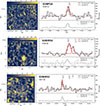 |
Fig. 4. Three most commonly detected H I lines across our sample. We show them using two of our regions. Left: Line moment-zero maps. The channels used to integrate the emission are those encompassed by the line Gaussian fits in the right panels. Red apertures enclose the map area used to extract the spectra at the protostars shown in the right panels (upper insets), while the broader grey aperture (minus the central red aperture) was used to extract the spectra of the local background (right panels, lower insets). Right: Gaussian curves fit the line emission for both the protostar (red, upper inset) and backgrounds (grey, lower insets). We reproduced the Gaussian fits of the background in upper insets to allow comparisons with the protostar Gaussian fit. For some of the lines (middle row), a second Gaussian is required for fitting another nearby emission line. Other detected lines are shown in Figures A.2, A.3, and A.4. |
A particular obscured case is the G28S protostellar source because it is undetected at all MIRI wavelengths, despite its association with a compact outflow (see Sect. 5.3). Conversely, G31 shows a bright outflow lobe in the continuum (Fig. 2, middle panel) and some H I emission lines (e.g. Fig. A.1), which makes it hard to study compact, accretion-driven emission on the source (Sect. 5.3). Lastly, IRAS18089 is the most difficult case to interpret as detailed in Appendix B.2. We do not report any detections towards the brightest protostar, IRAS18089 A; however, we cannot yet rule out that this emission actually exists.
4.4. Accretion parameters and luminosity from H I lines
Under the assumption that these compact detections are produced exclusively by accretion processes, one can convert their line luminosities, Lline, to accretion luminosities, Lacc (we discuss potential contaminants in Sect. 5.3). This is the first step to estimate accretion rates, but also the least trivial one because it requires appropriate empirical Lacc-calibrations. All lines included in Table 4, except H I 9–8, have an available Lacc- calibration. We nevertheless excluded H I 8–7 from further calculations because of the large uncertainty of its available calibration, especially at the higher LH I regimes we obtain. Although these calibrations have been established for low-mass, Class II objects, we still applied them to our sample of embedded, high-mass sources, and we discuss their validity with the Lacc results at hand.
We measured the luminosities of the four hydrogen lines of Table 4 that are detected to be compact, and Table 5 shows their Gaussian fitting parameters. The protostar’s S/N value is accompanied with that of the corresponding background in parentheses. When Lproto/Lbkg > 1, we used the luminosity difference to report line luminosities (Lline, obs =Lproto − Lbkg) in Table 5. We provide the extinction-corrected quantities (Lline, Lacc, and Ṁacc) in the last columns of Table 5. For Lacc and Ṁacc in particular, we provide all the possible values given the existing calibrations (when applicable). For these quantities, we also provide a second value immediately below, where the upper one was derived using the KP5 extinction curve and the lower one was derived using the M09 curve. We display Lacc in square brackets to indicate when they surpassed their region’s Lbol (Table 1); when they did not surpass Lbol, we report their corresponding accretion rates in the last three columns.
The H I line widths (FWHM in Table 5) range from velocities of 69–177 km s−1, where the MIRI spectral resolution corresponds to 100 km s−1 down to 80 km s−1 (Labiano et al. 2021); thus, some lines appear narrower than this resolution. There is no apparent correlation between specific lines and their widths. For instance, the compact detections of H I 6–5 towards G28P1 A and IRAS23385 A show contrasting FWHM of 69 (effectively an upper limit of 80 km s−1) and 164 km s−1, which could be indicative of different formation mechanisms. While the magnetospheric accretion scenario points to velocity widths from 150 km s−1 or more in Class II objects (Tofflemire et al. 2025) and IRAS23385 A is consistent with that threshold, it is still unclear what the correct velocity widths should be towards massive protostars as the exact physics of the accretion process might be different than that of low-mass, Class II objects.
4.5. H2O and OH lines
Water commonly shows several emission lines in the MIR spectra of Class II discs (e.g. Pontoppidan et al. 2010), where some appear at the wavelengths of H I emission lines such as H I 6–5, H I 7–6, and H I 12–7. For example, Shridharan et al. (2026) found high median water contamination for these lines in a sample of 79 Class II discs, meaning that the H I fluxes can be artificially enhanced if water emission is not taken into account. We therefore followed both Rigliaco et al. (2015) and Tofflemire et al. (2025) to determine whether water is contaminating any of our protostars by observing relatively bright, isolated lines at 11.648, 12.396, 14.428, 15.17, and 17.22 μm, where the one at 12.396 μm is very close to the H I 7–6 line.
We found no emission of these water lines with S/N ≥3 in our regions except by a single line at 14.428 μm in G28P1B, with a S/N of 5.8. However, among the lines we report for this particular region, the only detected line that can be affected by water is H I 7–6, for which the nearby water line at 12.396 μm is not seen (Fig. A.3). This makes this tentative detection of H I 7–6 unlikely to be affected by water. Apart from this particular case, the evidence shows, for the other regions, that water did not contaminate our reported H I line fluxes. We also note that the JOYS sample of low-mass, embedded sources (Class 0-I) show weaker lines (van Gelder et al. 2024a) than in the Class II sources of Rigliaco et al. (2015) and Shridharan et al. (2026).
We additionally searched for emission lines from the OH molecule, although with a different motivation. The OH molecule can potentially trace accretion because it might be generated in the interaction between the UV radiation produced at the shock and the water budget of the inner disc (Tabone et al. 2021). OH line emission was recently detected by tracing accretion (Watson et al. 2026), while in previous studies it was detected from outflows (Le Gouellec et al. 2025; Tychoniec et al. in prep.). Although there is currently no definitive method to quantify accretion luminosities or rates from OH, we tested whether OH is at least observed in our sample in favour of this outstanding debate. We searched for two quartets of OH lines at ∼16.0 and 16.8 μm and only found them in IRAS23385 A (as already reported in Francis et al. 2024). They appear spatially compact at the protostar, with low S/Ns, as shown in Fig. A.5. However, the fact that the four lines of each quartet are seen simultaneously provides certainty that the OH is present at the IRAS23385 A protostar.
4.6. Accretion rates
Our reported accretion rates in Table 5 are only tentative, because they are derived from Lacc estimations that already include important caveats (see discussion in Sect. 5.4). With this in mind, we provide a general overview here.
Given a Lacc value, accretion rates (Ṁacc) can be computed by solving Eq. (11.5) in Stahler & Palla (2004) for Ṁacc,
 (3)
(3)
for which the protostellar embryo mass, M★, and radius, R★, must be known. Within our sample, these stellar parameters are only known for IRAS23385 (M★ = 9 M⊙, R★ = 5 R⊙; Cesaroni et al. 2019). For the rest of the sources we can only use assumptions because existing (millimetre) observations for each region only provide the large-scale core (or clump) masses, which in addition tend to be located away from the actual IR core positions by at least a few arcseconds. We proceeded by adopting M★ = 5 M⊙ for all other sources, which is intended to represent sources that are still growing in mass and are bound to reach the 8 M⊙ or more. Subsequently, we adopted R★ = 9 R⊙ given the disc accretion model of Hosokawa et al. (2010), Figure 16) for the given stellar mass, and assuming an accretion rate of ∼ 10−5 M⊙ yr−1.
With the Shridharan et al. (2026) calibration providing most of our reported accretion luminosities in Table 5, tentative accretion rates range between ∼10−6 and 10−3 M⊙ yr−1 depending on the region, tracer, and dust-extinction model.
5. Discussion
5.1. H I line ratios compared to H I excitation models
In Fig. 5 we compare the luminosity ratios of the observed lines normalised to the Hu α line (when detected with S/N > 3) to Case B and CE models (see Sect. 1). We included two temperatures of 7500 and 104 K in separate panels in Fig. 5, and for the CE model in particular we included several densities. We find a large dispersion in the measured line ratios, for which the models can hardly constrain the particular conditions of temperature and density. Although few cases may be well fitted by the models (mainly G28P1B), it still depends on the adopted dust-extinction curve. For instance, the G28IRS2 protostar has both H I 7–6 and H I 8–6 lines detected with a good S/N (solid markers), but its LH I uncertainty given by the two extinction models of M09 and KP5 (circle and triangle, respectively) point to densities that are separated by orders of magnitude, namely higher than nH = 1012 cm−3 (using KP5) and lower than nH = 109 cm−3 (using M09).
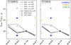 |
Fig. 5. Line ratios normalised to the Huα line, compared to the local excitation (KF11) and Case B models (Storey & Hummer 1995). Error bars are omitted, since the overall uncertainty is dominated by the discrepancy between the two extinction curves (triangle and circle markers). Solid markers represent detections with S/N > 5, while open markers show detections with 3< S/N < 5. Panels display models for temperatures of 10 000 K (left) and 7500 K (right), and for the KF11 model we also include different density values ranging from nH = 109 to 1012 cm−3. We show the Case B model for a single electron density value, Ne (in cm−3), as this parameter appears not to change predictions significantly. Lines in the x-axis are organised by increasing wavelength. |
Case B and CE models displayed in Fig. 5 also helped us to assess qualitative aspects of our detections in Table 4. They show that the H I 6–5 emissivity is expected to be higher than that of other α transitions (i.e. H I 7–6 and 8–7), regardless of the temperature (Case B and CE) or density (CE). On top of this, extinction curves indicate that H I 6–5 is the line least affected by extinction among those we detected here; hence, it should be enhanced compared to H I 7–6, for example. Despite these expectations, the luminosities LHI 6 − 5 are not among the highest, and the H I 7–6 line is found in at least the same number of cases. Following the same idea, for the two regions where both H I 6–5 and H I 7–6 lines are detected, we find the expected LHI 6 − 5> LHI 7 − 6 trend for three out of four measurements (two ratios per extinction curve), but the two H I 8–7 measurements for G28P1A are far above any model predictions.
Another interesting comparison involves both H I 6–5 and H I 8–6 as they are affected by very similar magnitudes of extinction due to their proximity in wavelength. Despite this mitigating the role of the adopted extinction model, their detections do not correlate well, because among the four regions where we detect at least one of them, the other is not detected in three cases. Part of the reason could be attributed to the low S/N of our detections, but on the other hand the CE model predicted inversions of the H I 6–5 to H I 8–6 flux ratio depending on density (Fig. 5). While for low densities (log(nH) ≲ 10) they predicted fluxes of FH I 6 − 5/FH I 8 − 6 > 1, for high densities (log(nH) ⪆ 12) they predicted FH I 6 − 5/FH I 8 − 6 < 1. This observed dispersion in line ratios involving H I 8–6 is therefore expected in the CE model, and it is a plausible scenario in which the volume density differences of our regions will be of a few orders of magnitude. More generally, the inconsistencies identified here (assuming that line emissivity models are correct) can be attributed to the low S/N of our observations; thus, more and deeper observations will be necessary to correctly assess these aspects.
5.2. The possibility of MIR H I lines tracing accretion in protostars
Our sample provides evidence that it is now possible to detect H I emission produced at the massive protostellar systems, refining the central questions to: what exactly produces this emission? Despite the accretion process being the most likely origin, there is still room for compact emission from the outflow (Sect. 5.3), winds, or, an (HC-)H II region.
Based on their detection rate, the lines best suited for the study of accretion in massive protostars seem to be H I 7–6, H I 6–5, and H I 8–6. However, the disagreement between available Lacc-calibrations currently limits their use. To illustrate this point, Fig. 6 shows, for the H I 7–6 line in particular, the distinct possible Lacc values given the three calibrations and given both the KP5 and M09 extinction curves. Both the Tofflemire et al. (2025) and Rigliaco et al. (2015) (solid black and blue lines) calibrations return unphysically high accretion luminosities, as they go above their respective Lbol (Table 1) in most cases. A more realistic picture is obtained with the Shridharan et al. (2026) calibrations, with many Lacc values below Lbol (14 cases out of 22, 9th column in Table 5), and some Lacc values above Lbol by factors of a few. In general, Figure 6 represents the cases of the H I 6–5 and H I 8–6 lines well.
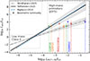 |
Fig. 6. Comparison of predicted Lacc (y-axis) given three calibrations established for the Hu α line and our measured line luminosities: LH I 7−6 (x-axis). The three curves reproduce these calibrations; the lower left box highlights the typical dynamical range over which they were derived, and the upper right box shows the contrasting line luminosity regimes of our sample, to which each calibration curve is extrapolated. The shaded areas correspond to the uncertainties of the Tofflemire et al. (2025) and Shridharan et al. (2026) calibrations. The coloured vertical lines show our measured LH I 7−6 values (Table 5), where two per region are displayed given the two M09 (dotted) and KP5 (dashed) extinction curves. Lbol values are indicated with triangles for each region, and corresponding LH I 7−6 are displayed up to eight times each region’s Lbol to give a sense of the maximum Lacc we can expect to still be physical (see Sect. 5.2). Error bars were omitted since the overall uncertainty is dominated by the two extinction curves. |
We note two aspects on existing Lbol measurements. (a) It is observationally possible that Lbol is lower than the total luminosity by factors of a few. The total- to bolometric-luminosity ratio, Ltot/Lbol, in a sample of Class 0/I/II objects increases with higher inclination angles and foreground extinction (Furlan et al. 2016). While inclination angles give median ratios from 1.5 to 3.5 (from low to high angles), Ltot/Lbol reaches up to 8.2 for sources with extinction AV > 50 mag, as was the case for most of our sources (we used this factor of 8 × Lbol as an upper limit in Fig. 6). Along the same line, Pokhrel et al. (2023) found similar ratios due to increasing inclination (∼1–10), and due to increasing extinction (2.1–6.1) for the Aquila and Orion clouds. In this scenario, Lacc might account for most of the protostar’s total luminosity by factors of a few, but it cannot explain the orders-of-magnitude differences that we often see given certain extinction model and Lacc-calibration combinations. (b) These Lbol measurements were obtained from larger spatial scales than those we used for our IR sources, which suggests that Lbol may be overestimated for our protostars (Lbol reported in Molinari et al. 2008 for IRAS23385; and in Urquhart et al. 2018 for the rest of our regions). Overall, these Lbol uncertainties did not allow our data to confidently rule out any specific Lacc-calibration, but the higher LH I cases strongly suggest that the relations of Rigliaco et al. (2015) and Tofflemire et al. (2025) do not apply in the higher mass regime’s sources.
The works presenting the luminosity calibrations followed different approaches to establish their relations. While Rigliaco et al. (2015) and Shridharan et al. (2026) obtained averaged curves from large samples, Tofflemire et al. (2025) studied a known binary system, benefiting from its predictable accretion-burst periods. Although this closely guarantees a precise characterisation of a single system, the work of Shridharan et al. (2026) counts with good self consistency between their different H I line relations. On the other hand, recent works have found that the mechanism driving accretion might change from Herbig Ae to Be stars (Donehew & Brittain 2011; Grant et al. 2022). Observations of Wichittanakom et al. (2020) and Vioque et al. (2022) have set a threshold of ∼4 M⊙ mass for these different accretion regimes, above which magnetospheric accretion might no longer be dominant (Ababakr et al. 2017). Currently, the boundary-layer mechanism is regarded as an alternative (described in Sect. 1); however, no observational evidence exists in favour of any proposed mechanism.
Regardless of the accretion mechanism, the hydrogen transition lines should always be produced by the accretion process; thus, they should trace the accretion luminosity provided the outflow contamination is not significant (and provided a hyper-compact H II region has not yet formed). Therefore, new calibrations focused on intermediate- to high-mass protostars have the potential to reveal accurate Lline to Lacc relations that can provide reliable accretion rates.
5.3. Contaminants: Outflows, diffuse emission, and (HC-)H II regions
Since accretion is not the only phenomenon producing H I lines, we identified all possible contaminants affecting our detections (see Table 4). We identified outflows based on the premise that if they are present, they should appear elongated (e.g. Fig. A.1). We also tested the presence of diffuse H I with an annulus around (or very close to) each protostar and determined whether (hyper-compact) H II regions are present from centimetre data in the literature.
Figure A.1 demonstrates that H I lines also trace outflows, in this case towards G31. The mosaic displays continuum-subtracted maps of G31 for five of the detected H I lines: H I 6–5, 8–6, 7–6, 8–7, and 10–7, and it includes two known tracers of outflow emission in the bottom row, the H2 0-0 (S1) and [Fe II] emission lines at 17.035 μm and 24.52 μm, respectively. In particular, it becomes clear that H I 6–5 and H I 7–6 are tracing extended emission that is consistent with that traced by H2 and [Fe II]. This comparison shows that the H I lines are not seen towards the driving source of G31, they are only coming from its outflow when detected. Ultimately, this implies that for compact H I line emission outflows can still contaminate the observed H I flux if the beam encompasses spatial scales larger than that of the immediate protostellar envelope. Since this is the case for the MIRI/MRS beam size towards our sources, outflow contamination cannot be fully ruled out for our detections.
Overall, outflows are present in the field of view of all the six regions, either traced in the MIR by H I lines (G31); H2 vibration lines (all regions); or in the millimetre regime by SiO (2–1) in G28IRS2 (Beuther et al. 2026), CO in G28P1 (Kong et al. 2019), SiO (2–1) and CO (2–1) in G28S (Tan et al. 2016; Feng et al. 2016b; Pillai et al. 2019), SiO (5–4) in IRAS18089 (Beuther et al. 2004), or both SiO (2–1) and HCO+(1–0) in IRAS23385 (Molinari et al. 1998b; Gieser et al. 2023). More generally, this also holds for low-mass sources, all of which show outflows and/or jets, yet a fraction come from accretion (shock conditions studied in Navarro et al. 2025). Future work will examine these JOYS outflows through H2, [Fe II], or [S I] lines, for example, and will quantify ejection rates as a complement to accretion rates.
Solid evidence for a hyper-compact H II region exists for IRAS18089 mm (e.g. Sridharan et al. 2002; Beuther et al. 2002c; Zapata et al. 2006), and sources of free-free emission are reported towards the millimetre peak of G31 (Cesaroni et al. 2010). In both cases, the centimetre emission data have an angular resolution comparable to our observations. The other regions were also studied at centimetre wavelengths, but no compact sources were detected (see Beuther et al. 2026 for the G28 sub-regions and Molinari et al. 1998a for IRAS23385).
5.4. Methodological caveats
Some important sources of uncertainty arise when attempting to quantify accretion rates for embedded massive protostars. The four main ones, ordered by decreasing importance according to our experience, are listed as follows:
-
(1)
The validity of empirical LHI to Lacc relations when extended to massive protostars.
-
(2)
The disagreement between available extinction curves in the literature, especially at wavelengths around the broad silicate absorption feature that peaks at 9.7 μm.
-
(3)
The estimation of τ9.7.
-
(4)
Stellar parameters: mass and radius of the protostellar embryo.
We elaborate on each point in the following. Regarding caveat (1), it remains unclear how valid it is to extrapolate calibrations established for low-mass Class II objects to massive protostars that actually show much higher Lline. In line with our findings, the works suggesting that the accretion mechanism might vary for higher stellar masses (from ∼4 M⊙, Sect. 5.2) strongly motivates the development of new calibrations adapted to these higher mass regimes, for which MIRI-MRS would be critical. A feasible approach would be to search for several intermediate- to high-mass sources with known accretion parameters (measured using tracers in the near-IR). Alternatively, contemporaneous measurements of MIR H I tracers and Lacc can mitigate the uncertainty given by accretion variability. Crucially, the possibility to use H I lines as tracers of accretion luminosity remains unaltered despite this caveat.
Concerning caveat (2), the two dust-extinction models we implemented in this work can provide contrasting factors depending on wavelength; therefore, H I lines are unequally affected and conclusions become harder to extract. The clearest evidence of this is the factor of ∼1.6 difference that separates the extinction of H I 7–6 (12.37 μm) measured using the KP5 and M09 curves (Table 3). More generally, Table 5 shows the two possible luminosities for each line, reflecting how each of them is affected. From this particular perspective, H I 6–5 and H I 8–6 gain more reliability as the dust extinction curves differ less at their wavelengths.
Moving to caveat (3), the fitting results still depend on which absorbing species are considered. Although water ice and silicates seem to be dominant, our fits achieve different levels of accuracy. Similarly, the wavelength ranges provided to the fitter as input also affect the results. Since the main absorption feature at 9.7 μm goes deeper than the noise floor for all our sources, we miss a relevant fraction of both the slope at R2, and the bluer tip of R3. To conclude, incorporating more absorbing species (e.g. HCOOH, CO2) and possibly the PAH emission feature, together with deeper observations of the main silicate feature, has the potential to yield more accurate fits. Alternatively, Chen et al., in prep. provides a complementary approach to modelling protostellar spectra.
Caveat (4) arises at the last step, affecting only accretion rates. Indeed, stellar parameters are frequently unknown for the most embedded stages as their envelopes tend to be more massive. However, promising progress has been made to estimate embedded protostellar masses using NOEMA or ALMA from molecular line kinematics of young discs. Although mostly done for sources closer than ∼400 pc (Lee et al. 2017; Tobin & Sheehan 2024), where masses reach up to 2.6 M⊙ (Ohashi et al. 2023), measurements on massive protostars have been achieved at distances of 2 kpc, pointing to masses up to 25 M⊙ (Ahmadi et al. 2023). New observations with existing facilities can potentially provide clarity on the stellar parameters towards the (usually kiloparsec-distant) high-mass protostars.
In addition to these caveats, we emphasise that a difficult-to-quantify fraction of the compact emission may come from outflows in more cases than we report here (see discussion in Sect. 5.3).
6. Conclusions
We performed the first accretion-focused JWST study for a sample of high-mass star-forming regions, extending from the better-known low-mass Class II objects to explore the less understood massive protostellar objects. We searched for compact emission from hydrogen transitions; we unveiled the potential stumbling blocks for any similar study, and therefore we show what the prospects can be, given current instruments, of actually measuring accretion rates onto massive protostars. Our conclusions are the following:
-
Hydrogen emission lines in the MIR can now be detected systematically using MIRI/JWST, although care should be taken to understand what processes are actually driving the emission. Besides accretion, outflows, hyper-compact H II regions, and environmental diffuse gas can produce H I emission lines.
-
Three emission lines of hydrogen stand out because of their detection rate, which places them as the best candidate tracers of protostellar accretion for massive protostars. These lines are H I 7–6, H I 6–5, and H I 8–6.
-
Our accretion luminosity estimations carry large uncertainties, which limits the informative value of the accretion rates. For that reason, and because the accretion process is believed to change for stars more massive than ∼4 M⊙, this work reveals the need to develop LH I- to Lacc-calibrations focused on higher mass objects. For such a calibration to yield physical Lacc for intermediate- to high-mass protostars given typical Lbol values, we anticipate a shallower growth of Lacc with Lline compared to what has been derived for low-mass T-Tauri stars.
-
We emphasise (and largely describe) throughout this work the role of uncertainties propagated in each step. Importantly, our approach to estimate extinctions, AK (see Gieser et al. 2026), represents a step forward, because it offers solid constraints for at least some of our sources. Ultimately, this brings us closer to achieving systematic characterisations of extincted emission due to massive envelopes.
Accretion rates in high-mass protostars remain challenging; however, this work contributes to outlining the limitations of current work and possible pathways, given the potential of the JWST, to better understand accretion processes in high-mass protostars.
Acknowledgments
This work is based on observations made with the NASA/ESA/CSA James Webb Space Telescope. The data were obtained from the Mikulski Archive for Space Telescopes at the Space Telescope Science Institute, which is operated by the Association of Universities for Research in Astronomy, Inc., under NASA contract NAS 5-03127 for JWST. These observations are associated with program 1290. This work is based in part on observations made with the Spitzer Space Telescope, which was operated by the Jet Propulsion Laboratory, California Institute of Technology under a contract with NASA. This paper makes use of the following ALMA data: ADS/JAO.ALMA# 2017.1.00101.S, 2013.1.00489.S, 2019.1.00195.L and 2011.0.00429.S. ALMA is a partnership of ESO (representing its member states), NSF (USA) and NINS (Japan), together with NRC (Canada), NSTC and ASIAA (Taiwan), and KASI (Republic of Korea), in cooperation with the Republic of Chile. The Joint ALMA Observatory is operated by ESO, AUI/NRAO and NAOJ. The Submillimeter Array is a joint project between the Smithsonian Astrophysical Observatory and the Academia Sinica Institute of Astronomy and Astrophysics and is funded by the Smithsonian Institution and the Academia Sinica. A.C.G. acknowledges support from PRIN-MUR 2022 20228JPA3A “The path to star and planet formation in the JWST era (PATH)” funded by NextGeneration EU and by INAF-GoG 2022 “NIR-dark Accretion Outbursts in Massive Young stellar objects (NAOMY)” and Large Gran INAF-2024 “Spectral Key fea-tures of Young stellar objects: Wind-Accretion LinKs Explored in the infraRed (SKYWALKER)”. V.J.M.L.G. acknowledges support by the Unidad de Excelencia María de Maeztu program number CEX2020-001058-M. V.J.M.L.G. acknowledges support by the European Research Council (ERC) under the European Union’s Horizon 2020 research and innovation program (grant agreement No. 101098309 – PEBBLES).
References
- Ababakr, K. M., Oudmaijer, R. D., & Vink, J. S. 2017, MNRAS, 472, 854 [NASA ADS] [CrossRef] [Google Scholar]
- Ahmadi, A., Beuther, H., Bosco, F., et al. 2023, A&A, 677, A171 [NASA ADS] [CrossRef] [EDP Sciences] [Google Scholar]
- Alcalá, J. M., Natta, A., Manara, C. F., et al. 2014, A&A, 561, A2 [NASA ADS] [CrossRef] [EDP Sciences] [Google Scholar]
- Arce, H. G., Shepherd, D., Gueth, F., et al. 2007, in Protostars and Planets V, eds. B. Reipurth, D. Jewitt, & K. Keil, 245 [Google Scholar]
- Baker, J. G., & Menzel, D. H. 1938, ApJ, 88, 52 [Google Scholar]
- Beltrán, M. T., Cesaroni, R., Rivilla, V. M., et al. 2018, A&A, 615, A141 [Google Scholar]
- Beuther, H., Schilke, P., Menten, K. M., et al. 2002a, ApJ, 566, 945 [Google Scholar]
- Beuther, H., Schilke, P., Sridharan, T. K., et al. 2002b, A&A, 383, 892 [NASA ADS] [CrossRef] [EDP Sciences] [Google Scholar]
- Beuther, H., Walsh, A., Schilke, P., et al. 2002c, A&A, 390, 289 [NASA ADS] [CrossRef] [EDP Sciences] [Google Scholar]
- Beuther, H., Hunter, T. R., Zhang, Q., et al. 2004, ApJ, 616, L23 [NASA ADS] [CrossRef] [Google Scholar]
- Beuther, H., Mottram, J. C., Ahmadi, A., et al. 2018, A&A, 617, A100 [NASA ADS] [CrossRef] [EDP Sciences] [Google Scholar]
- Beuther, H., van Dishoeck, E. F., Tychoniec, L., et al. 2023, A&A, 673, A121 [NASA ADS] [CrossRef] [EDP Sciences] [Google Scholar]
- Beuther, H., Kuiper, R., & Tafalla, M. 2025, ARA&A, 63, 1 [Google Scholar]
- Beuther, H., Gieser, C., Linz, H., et al. 2026, A&A, 706, A329 [NASA ADS] [CrossRef] [EDP Sciences] [Google Scholar]
- Bhandare, A., Ali Ahmad, A., & Commerçon, B. 2025, A&A, 702, L7 [NASA ADS] [CrossRef] [EDP Sciences] [Google Scholar]
- Boogert, A. C. A., Chiar, J. E., Knez, C., et al. 2013, ApJ, 777, 73 [NASA ADS] [CrossRef] [Google Scholar]
- Bouvier, J., Alencar, S. H. P., Boutelier, T., et al. 2007, A&A, 463, 1017 [NASA ADS] [CrossRef] [EDP Sciences] [Google Scholar]
- Cesaroni, R., Olmi, L., Walmsley, C. M., Churchwell, E., & Hofner, P. 1994, ApJ, 435, L137 [NASA ADS] [CrossRef] [Google Scholar]
- Cesaroni, R., Hofner, P., Araya, E., & Kurtz, S. 2010, A&A, 509, A50 [NASA ADS] [CrossRef] [EDP Sciences] [Google Scholar]
- Cesaroni, R., Beuther, H., Ahmadi, A., et al. 2019, A&A, 627, A68 [EDP Sciences] [Google Scholar]
- Csengeri, T., Leurini, S., Wyrowski, F., et al. 2016, A&A, 586, A149 [NASA ADS] [CrossRef] [EDP Sciences] [Google Scholar]
- Donehew, B., & Brittain, S. 2011, AJ, 141, 46 [Google Scholar]
- Dunham, M. M., Allen, L. E., Evans, N. J., II., et al. 2015, ApJS, 220, 11 [NASA ADS] [CrossRef] [Google Scholar]
- Edwards, S., Kwan, J., Fischer, W., et al. 2013, ApJ, 778, 148 [NASA ADS] [CrossRef] [Google Scholar]
- Feng, S., Beuther, H., Zhang, Q., et al. 2016a, A&A, 592, A21 [NASA ADS] [CrossRef] [EDP Sciences] [Google Scholar]
- Feng, S., Beuther, H., Zhang, Q., et al. 2016b, ApJ, 828, 100 [Google Scholar]
- Franceschi, R., Henning, T., Tabone, B., et al. 2024, A&A, 687, A96 [NASA ADS] [CrossRef] [EDP Sciences] [Google Scholar]
- Francis, L., van Gelder, M. L., van Dishoeck, E. F., et al. 2024, A&A, 683, A249 [NASA ADS] [CrossRef] [EDP Sciences] [Google Scholar]
- Frank, A., Ray, T. P., Cabrit, S., et al. 2014, in Protostars and Planets VI, eds. H. Beuther, R. S. Klessen, C. P. Dullemond, & T. Henning, 451 [Google Scholar]
- Furlan, E., Fischer, W. J., Ali, B., et al. 2016, ApJS, 224, 5 [Google Scholar]
- Gieser, C., Beuther, H., van Dishoeck, E. F., et al. 2023, A&A, 679, A108 [NASA ADS] [CrossRef] [EDP Sciences] [Google Scholar]
- Gieser, C., Rocha, W. R. M., Chen, Y., et al. 2026, A&A, in press, https://doi.org/10.1051/0004-6361/202558615 [Google Scholar]
- Grant, S. L., Espaillat, C. C., Brittain, S., Scott-Joseph, C., & Calvet, N. 2022, ApJ, 926, 229 [NASA ADS] [CrossRef] [Google Scholar]
- Gullbring, E., Calvet, N., Muzerolle, J., & Hartmann, L. 2000, ApJ, 544, 927 [NASA ADS] [CrossRef] [Google Scholar]
- Hamann, F., & Persson, S. E. 1992, ApJS, 82, 247 [NASA ADS] [CrossRef] [Google Scholar]
- Hartmann, L. 2008, Accretion Processes in Star Formation [Google Scholar]
- Hartmann, L., Herczeg, G., & Calvet, N. 2016, ARA&A, 54, 135 [Google Scholar]
- Hosokawa, T., Yorke, H. W., & Omukai, K. 2010, ApJ, 721, 478 [Google Scholar]
- Hummer, D. G., & Storey, P. J. 1987, MNRAS, 224, 801 [NASA ADS] [CrossRef] [Google Scholar]
- Koenigl, A. 1991, ApJ, 370, L39 [Google Scholar]
- Kong, S., Arce, H. G., Maureira, M. J., et al. 2019, ApJ, 874, 104 [Google Scholar]
- Kwan, J., & Fischer, W. 2011, MNRAS, 411, 2383 [Google Scholar]
- Labiano, A., Argyriou, I., Álvarez-Márquez, J., et al. 2021, A&A, 656, A57 [NASA ADS] [CrossRef] [EDP Sciences] [Google Scholar]
- Le Gouellec, V. J. M., Lew, B. W. P., Greene, T. P., et al. 2025, ApJ, 985, 225 [Google Scholar]
- Lee, C.-F., Ho, P. T. P., Li, Z.-Y., et al. 2017, Nat. Astron., 1, 0152 [CrossRef] [Google Scholar]
- Lynden-Bell, D., & Pringle, J. E. 1974, MNRAS, 168, 603 [Google Scholar]
- McClure, M. 2009, ApJ, 693, L81 [NASA ADS] [CrossRef] [Google Scholar]
- Molinari, S., Brand, J., Cesaroni, R., Palla, F., & Palumbo, G. G. C. 1998a, A&A, 336, 339 [NASA ADS] [Google Scholar]
- Molinari, S., Testi, L., Brand, J., Cesaroni, R., & Palla, F. 1998b, ApJ, 505, L39 [NASA ADS] [CrossRef] [Google Scholar]
- Molinari, S., Faustini, F., Testi, L., et al. 2008, A&A, 487, 1119 [NASA ADS] [CrossRef] [EDP Sciences] [Google Scholar]
- Molinari, S., Schilke, P., Battersby, C., et al. 2025, A&A, 696, A149 [NASA ADS] [CrossRef] [EDP Sciences] [Google Scholar]
- Muzerolle, J., Hartmann, L., & Calvet, N. 1998, AJ, 116, 455 [Google Scholar]
- Navarro, M. G., Nisini, B., Giannini, T., et al. 2025, ApJ, 995, 199 [Google Scholar]
- Ohashi, N., Tobin, J. J., Jørgensen, J. K., et al. 2023, ApJ, 951, 8 [NASA ADS] [CrossRef] [Google Scholar]
- Palla, F., & Stahler, S. W. 1999, ApJ, 525, 772 [NASA ADS] [CrossRef] [Google Scholar]
- Pillai, T., Kauffmann, J., Zhang, Q., et al. 2019, A&A, 622, A54 [NASA ADS] [CrossRef] [EDP Sciences] [Google Scholar]
- Pokhrel, R., Megeath, S. T., Gutermuth, R. A., et al. 2023, ApJS, 266, 32 [NASA ADS] [CrossRef] [Google Scholar]
- Pontoppidan, K. M., Salyk, C., Blake, G. A., & Käufl, H. U. 2010, ApJ, 722, L173 [NASA ADS] [CrossRef] [Google Scholar]
- Pontoppidan, K. M., Evans, N., Bergner, J., & Yang, Y.-L. 2024, Res. Notes Am. Astron. Soc., 8, 68 [Google Scholar]
- Rigliaco, E., Natta, A., Testi, L., et al. 2012, A&A, 548, A56 [NASA ADS] [CrossRef] [EDP Sciences] [Google Scholar]
- Rigliaco, E., Pascucci, I., Duchene, G., et al. 2015, ApJ, 801, 31 [Google Scholar]
- Rocha, W. R. M., van Dishoeck, E. F., Ressler, M. E., et al. 2024, A&A, 683, A124 [NASA ADS] [CrossRef] [EDP Sciences] [Google Scholar]
- Rogers, C., de Marchi, G., & Brandl, B. 2025, A&A, 698, A172 [NASA ADS] [CrossRef] [EDP Sciences] [Google Scholar]
- Salyk, C., Herczeg, G. J., Brown, J. M., et al. 2013, ApJ, 769, 21 [CrossRef] [Google Scholar]
- Sanhueza, P., Girart, J. M., Padovani, M., et al. 2021, ApJ, 915, L10 [NASA ADS] [CrossRef] [Google Scholar]
- Shepherd, D. S., & Churchwell, E. 1996a, ApJ, 472, 225 [NASA ADS] [CrossRef] [Google Scholar]
- Shepherd, D. S., & Churchwell, E. 1996b, ApJ, 457, 267 [NASA ADS] [CrossRef] [Google Scholar]
- Shridharan, B., Manoj, P., Pathak, V. C., et al. 2026, A&A, 708, A22 [NASA ADS] [CrossRef] [EDP Sciences] [Google Scholar]
- Sridharan, T. K., Beuther, H., Schilke, P., Menten, K. M., & Wyrowski, F. 2002, ApJ, 566, 931 [Google Scholar]
- Stahler, S. W., & Palla, F. 2004, The Formation of Stars [Google Scholar]
- Storey, P. J., & Hummer, D. G. 1995, MNRAS, 272, 41 [NASA ADS] [CrossRef] [Google Scholar]
- Tabone, B., van Hemert, M. C., van Dishoeck, E. F., & Black, J. H. 2021, A&A, 650, A192 [NASA ADS] [CrossRef] [EDP Sciences] [Google Scholar]
- Tan, J. C., Kong, S., Zhang, Y., et al. 2016, ApJ, 821, L3 [Google Scholar]
- Tobin, J. J., & Sheehan, P. D. 2024, ARA&A, 62, 203 [NASA ADS] [CrossRef] [Google Scholar]
- Tofflemire, B. M., Manara, C. F., Banzatti, A., et al. 2025, ApJ, 985, 224 [Google Scholar]
- Urquhart, J. S., König, C., Giannetti, A., et al. 2018, MNRAS, 473, 1059 [Google Scholar]
- van Dishoeck, E. F., Tychoniec, Ł., Rocha, W. R. M., et al. 2025, A&A, 699, A361 [NASA ADS] [CrossRef] [EDP Sciences] [Google Scholar]
- van Gelder, M. L., Francis, L., van Dishoeck, E. F., et al. 2024a, A&A, 692, A197 [NASA ADS] [CrossRef] [EDP Sciences] [Google Scholar]
- van Gelder, M. L., Ressler, M. E., van Dishoeck, E. F., et al. 2024b, A&A, 682, A78 [NASA ADS] [CrossRef] [EDP Sciences] [Google Scholar]
- Vioque, M., Oudmaijer, R. D., Wichittanakom, C., et al. 2022, ApJ, 930, 39 [NASA ADS] [CrossRef] [Google Scholar]
- Wang, Y., Zhang, Q., Pillai, T., Wyrowski, F., & Wu, Y. 2008, ApJ, 672, L33 [NASA ADS] [CrossRef] [Google Scholar]
- Watson, D. M., Narang, M., Pittman, C. V., et al. 2026, ApJ, 999, 264 [Google Scholar]
- Wichittanakom, C., Oudmaijer, R. D., Fairlamb, J. R., et al. 2020, MNRAS, 493, 234 [Google Scholar]
- Xu, Y., Moscadelli, L., Reid, M. J., et al. 2011, ApJ, 733, 25 [NASA ADS] [CrossRef] [Google Scholar]
- Zapata, L. A., Rodríguez, L. F., Ho, P. T. P., Beuther, H., & Zhang, Q. 2006, AJ, 131, 939 [NASA ADS] [CrossRef] [Google Scholar]
- Zhang, Q., Wang, K., Lu, X., & Jiménez-Serra, I. 2015, ApJ, 804, 141 [Google Scholar]
Appendix A: Detailed H I line detections
In the following we dive deeper into each line detection, highlighting important aspects of their derived parameters, including caveats, with the purpose of enabling further interpretations of how much they can be used to constrain accretion parameters toward massive protostars (Sect. 5.2).
Humphreysα (H I 7−6): it is the most frequently detected line in the sample of Rigliaco et al. (2015), which remains true in our smaller sample despite Hu α being strongly affected by the silicate absorption feature at 9.7 μm. Among our four detections, that of G28IRS2 stands out with S/N = 7.4 (Fig. 4, third row), and with a protostar emission about 1.6 times brighter than that of the local background, making it a relatively secure detection. In this case, the neighbor line HI(11−8) is never detected. G28P1 A and B show tentative detections, but G28P1 B is detected only 1% above the background (Lproto/Lbkg = 1.01), hence it is the least secure detection of all. Lastly, IRAS23385 A is fitted with S/N of 2.5, while its local background shows no emission. We can compare the latter result toward IRAS23385 A with that of Beuther et al. (2023), who report a tentative detection with S/N ∼3. There are key differences because they used an aperture of 2″ radius that encompass both IRAS23385 A and B, but since IRAS23385 A is the sole driver of compact ionization we centered the aperture at this protostar only, adopting a smaller aperture of 0.″5 (same for all our regions). Their larger aperture adds emission from H I 11–8, which is particularly seen diffuse in IRAS23385, and whose flux has to be summed to that of H I 7–6 when applying the calibration of Rigliaco et al. (2015) (as pointed out in Franceschi et al. 2024). All of these explain our lower S/N of 2.5. Our integrated line luminosity is lower, however, as we measured a 2.2 times higher AK extinction (likely due to our smaller aperture size), our Lacc becomes ∼5 times higher (using same dust extinction model). Overall, our lower S/N reduces the certainty of the H I 7–6 detection, however, the copious H I 6 − 5 and H I 8 − 6 compact emission confirms the presence of ionizing activity at the IRAS23385 A source.
Pfundα (H I 6−5): It is detected in two protostars with S/N > 4.5 and significant Lproto/Lbkg ratio (Table 5). The line is also detected as an outflow in G31 due to its very extended emission, and toward IRAS18089mm, which is probably an HC-H II region since 0.7, 1.3, and 3.6 cm emission is detected with spectral index of 0.58 (Sridharan et al. 2002; Beuther et al. 2004; Zapata et al. 2006), indicative of a slightly compact, optically thick region with free free emission.
Humphreysβ (H I 8−6): It is detected in three protostars as compact emission, with no diffuse environment contamination in two cases. Two line detections deserve small comments regarding their validity. The G28IRS2 detection has a high S/N of 8.7, however its Gaussian peak appears slightly redshifted by about 1.5 channels (i.e. ∼48 kms−1), which does not seem to be a detector issue because the line at the background appears where expected given the G28 vlsr as shown in Fig. 4 (second row, lower inset). The second gaussian component appears two channels blueshifted (i.e. -64 kms−1) with respect to the H I 11–7 line (upper inset), and it is less clear that it actually corresponds to this H I transition. Despite this note, we assume this is a true detection and we include it in Table 5. On the other hand, the integrated line map of IRAS23385 A in Fig. A.2 shows some extended structure that may resemble that of outflows, but none of that emission reaches a S/N of 2.5, therefore we treat it as a compact detection produced by accretion.
H I10−7: We have two tentative detections with no diffuse contamination nor extended emission associated to outflows. However, we judged them as dubious because that of G28P1B appears two channels blueshifted (−64 kms−1) given its vlsr , and that of IRAS18089C has a narrow baseline that affects the noise measurement (Appendix B.2). For these reasons they are flagged in Tables 4 and 5, and excluded from the analyses of Sect. 5.
A.1. Studied H I transitions
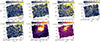 |
Fig. A.1. Integrated map of H I lines and the outflow tracer lines H2 (17.03 μm) and [Fe II] (24.52 μm) in the G31 region. White contours show ALMA 1.3 mm continuum. The contrasting emission of the outflow tracers demonstrate that, for this region, the H I lines are mainly produced along the outflow (see Table 4). |
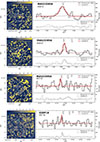 |
Fig. A.2. Continuation of Fig. 4 for IRAS23385 (H I transitions 6–5, 8–6, 7–6) and G28P1A (H I 7–6). Left: line moment 0 maps. The channels used to integrate the emission are those encompassed by the line Gaussian fits in the right panels. Red apertures enclose the map area used to extract the spectra at the protostars shown in right panels (upper insets), while the broader grey aperture (minus the central red aperture) is used to extract the spectra of the local background (right panels, lower insets). Right: Gaussian curves fit the line emission for both protostar (red, upper inset) and backgrounds (grey, lower insets). We reproduce the Gaussian fits of the background in upper insets to allow comparisons with the protostar Gaussian fit. |
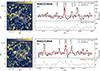 |
Fig. A.5. Detection of OH emission in IRAS23385 A. We include a single-component Gaussian fit to the central line, which is a narrow blend of the two central lines in each OH quartet. |
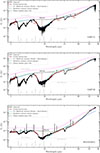 |
Fig. A.6. Continuation of Figure 3. Full MIRI spectrum of the labeled protostars (black). It shows several absorption features, where the broader one at 9.7 μm is produced by silicate grains. Two blackbody components absorbed by silicates and H2O are fitted to reproduce the overall continuum. The blue curve represents the fit obtained by considering those spectral ranges that are predominantly absorbed by silicates and H2O (in red, also indicated by the R1-R4 anchor ranges in top panel). The green curve shows the modeled blackbody emission only absorbed by silicates, while the dotted magenta curve shows the modeled blackbody emission unaffected by absorption. The black dashed curve above the main silicate absorption feature at 9.7 μm is an interpolation of the silicate-absorbed continuum from a polynomial fit. Here, the red vertical line highlights the resulting depth of the feature that determines τ9.7, whose uncertainty is given by the other two polynomial fits passing above and below (grey curves). The black dashed line at R4 indicates the location of the secondary silicate absorption feature. |
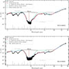 |
Fig. A.7. Continuation of Figure 3. For IRAS18089 A and C we masked the very deep absorption features at 5.9 and 6.9 μm as it shows mostly noise. |
All H I transitions considered in this work.
Fitted parameters from the spectrum of each IR source.
Appendix B: Post-Processing Steps
B.1. Astrometric correction
To correct the astrometry of all our data cubes we retrieved from the MAST portal (already reduced) parallel MIRI images and point-source catalogues for five of our sources − only for G28P1 these level 3 data products were not available. We found Gaia sources matching catalogued MIRI sources for only three of the regions. Within 0.5" they are G31 (10 matches), G29IRS2 (4 matches), and G28S (4 matches). Their relative astrometric shifts are ΔRA = 100.7 and ΔDEC = 27.0 mas for G31; ΔRA = 158.0 and ΔDEC = 15.26 mas for G28IRS2; and ΔRA = 141.9 and ΔDEC = 61.4 mas for G28S. Despite the small number of Gaia-MIRI counterparts, their shifts in RA and DEC are consistent among the three regions, confirming that the astrometric difference in the pointing of JWST to Gaia is in fact systematic.
We applied the individual shifts we found to equally correct each corresponding region. Particular cases are the following. G28P1 (the only region without image in MAST) is located in the same molecular cloud as G28IRS2 and G28S and it was observed on the same run within a few hours difference. Hence, we assumed they are equally affected by the JWST pointing and we assigned to it a shift that is the average between the former two, namely 150 and 38 mas in RA and DEC respectively. For IRAS23385 we used the correction that was already obtained in Beuther et al. (2023), where they used again the MIRI images at 15 μm to compare − uncatalogued − MIRI point sources to Gaia (corresponding 15 μm image in van Dishoeck et al. 2025, Fig. C.1). Finally, for IRAS18089 we tried the later approach, but we only found one Gaia source that matched a MIRI point source. Together with the fact that the corresponding shift was very small (less than 100 mas) we did not apply a pointing correction to IRAS18089.
B.2. Continuum subtraction: the IRAS18089 case
We describe first the issues we encountered when creating continuum-subtracted maps for IRAS18089, and secondly the extra steps we applied to mitigate them. The very high contrast in brightness between IR-source and background pixels in IRAS18089 produces, at the IR bright pixels, significant flux excess (or flux loss) after the continuum subtraction due to the − unavoidable although small − difference of the polynomial fit relative to the real continuum. In other words, at the brightest pixels the flux difference of the real continuum and the misfitted polynomial will still be much higher than the background noise level, making those pixels appear very bright (or very dark) on our maps depending on whether the fit missed the continuum from below (or above). This in turn produces "chequered" patterns in the integrated intensity maps that make them difficult to analyze.
To maximize the fit precision we narrowed the spectral range used to fit the polynomials, leaving only seven channels on each side of the masked spectrum, although at the expense of a more accurate noise estimate. Figure B.1 illustrates how the continuum subtraction works. Pixel spectra tend to follow flat, curved, or wiggled shapes, hence fitting simultaneously three polynomials (order 1, 2, and 3) to each pixel ensures that each case will be modeled. On a parallel track, we encountered single channels with relevant flux looses. They appear in several bright pixels at the IRAS18089 source locations, making the continuum subtraction imprecise (see right panel in Fig. B.1). As these single-channel bowls are artifacts, we masked them from our data cubes on a 5 sigma detection basis prior to fitting the continuum, while assigning them instead the average value of the few neighbor pixel channels. Lastly, we applied a 1D fringe correction using the python package jwst.residual_fringe.utils, although its correcting effect is minor as it reduces fringing at scales that are larger than those used in our fittings.
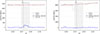 |
Fig. B.1. Examples of continuum subtraction on two adjacent, high-flux pixels at the IR source A of IRAS18089 that show contrasting behaviors. The pixel spectrum of the left panel displays the Humphreys alpha line, while the spectrum on the right panel shows a deep artifact that we masked prior to the fitting (red line). In this case the artifact consists of two contiguous, negative channels, where the deeper one is capable of deviating the polynomial fit significantly. The shaded area highlights the spectral range that was excluded when fitting the continuum. The left panel is, at the same time, a good representation of how the continuum subtraction works for the remaining five regions as they do not show negative artifacts. The vertical lines show the nominal wavelength of the Hu α line. |
All Tables
All Figures
|
Fig. 1. Overview of three less evolved regions of our sample: G28IRS2, G28P1, and G28S. In this case, all of them belong to the same IRDC G28. Left: Spitzer (8 μm) view of the whole IRDC G28. The three target sub-regions are depicted with millimetre contours (white) from ALMA for G28IRS2 (Molinari et al. 2025) and G28P1 (Zhang et al. 2015), and from SMA for G28S (Feng et al. 2016a), with cyan boxes highlighting the field of view of our MIRI observations, which are slightly magnified for better visualisation. Middle and right panels: Zoomed-in views of the target sub-regions. These show the MIRI continuum at 14 μm, whereas cyan contours trace the continuum at 5 μm (no IR source was detected towards G28S). The ellipses in the bottom right corners represent beam sizes: grey for the 14 μm image and cyan for the 5 μm contours. |
| In the text | |
|
Fig. 2. Overview of three more evolved protostellar regions of our sample: IRAS18089, G31, and IRAS23385. Top panels: Each region as seen by Spitzer (3.6 μm) or WISE (12 μm), with white contours depicting millimetre data from ALMA for IRAS18089 (1.2 mm; Sanhueza et al. 2021) and G31 (1.3 mm; Beltrán et al. 2018), or NOEMA for IRAS23385 (1 mm; Beuther et al. 2018). The cyan boxes highlight the field of view of our MIRI observations. Bottom panels: MIRI integrated images at 14 μm for each region covering the corresponding upper panels. The cyan contours represent the continuum at 5 μm. |
| In the text | |
|
Fig. 3. Full MIRI spectrum of the G28IRS2 protostar (black). It shows several absorption features, where the broader one at 9.7 μm is produced by silicate grains. Blackbody components (3 in this case) absorbed by silicates and H2O were fitted to reproduce the overall continuum. The blue curve represents the fit obtained by considering spectral ranges that are predominantly absorbed by silicates and H2O (in red, also indicated by the R1–R4 ranges). The green curve represents blackbody emission that would only be absorbed by silicates, while the dotted magenta curve shows the modelled blackbody emission unaffected by absorption. The dashed black curve above the main silicate absorption feature at 9.7 μm is an interpolation of the silicate-absorbed continuum from a five-order polynomial fit. Here, the vertical red line highlights the resulting depth of the feature that determines τ9.7, whose uncertainty is given by another two polynomials (of the order of 1 and 4) fits passing above and below (grey curves). The dashed black line at R4 indicates the location of the secondary silicate absorption feature. |
| In the text | |
|
Fig. 4. Three most commonly detected H I lines across our sample. We show them using two of our regions. Left: Line moment-zero maps. The channels used to integrate the emission are those encompassed by the line Gaussian fits in the right panels. Red apertures enclose the map area used to extract the spectra at the protostars shown in the right panels (upper insets), while the broader grey aperture (minus the central red aperture) was used to extract the spectra of the local background (right panels, lower insets). Right: Gaussian curves fit the line emission for both the protostar (red, upper inset) and backgrounds (grey, lower insets). We reproduced the Gaussian fits of the background in upper insets to allow comparisons with the protostar Gaussian fit. For some of the lines (middle row), a second Gaussian is required for fitting another nearby emission line. Other detected lines are shown in Figures A.2, A.3, and A.4. |
| In the text | |
|
Fig. 5. Line ratios normalised to the Huα line, compared to the local excitation (KF11) and Case B models (Storey & Hummer 1995). Error bars are omitted, since the overall uncertainty is dominated by the discrepancy between the two extinction curves (triangle and circle markers). Solid markers represent detections with S/N > 5, while open markers show detections with 3< S/N < 5. Panels display models for temperatures of 10 000 K (left) and 7500 K (right), and for the KF11 model we also include different density values ranging from nH = 109 to 1012 cm−3. We show the Case B model for a single electron density value, Ne (in cm−3), as this parameter appears not to change predictions significantly. Lines in the x-axis are organised by increasing wavelength. |
| In the text | |
|
Fig. 6. Comparison of predicted Lacc (y-axis) given three calibrations established for the Hu α line and our measured line luminosities: LH I 7−6 (x-axis). The three curves reproduce these calibrations; the lower left box highlights the typical dynamical range over which they were derived, and the upper right box shows the contrasting line luminosity regimes of our sample, to which each calibration curve is extrapolated. The shaded areas correspond to the uncertainties of the Tofflemire et al. (2025) and Shridharan et al. (2026) calibrations. The coloured vertical lines show our measured LH I 7−6 values (Table 5), where two per region are displayed given the two M09 (dotted) and KP5 (dashed) extinction curves. Lbol values are indicated with triangles for each region, and corresponding LH I 7−6 are displayed up to eight times each region’s Lbol to give a sense of the maximum Lacc we can expect to still be physical (see Sect. 5.2). Error bars were omitted since the overall uncertainty is dominated by the two extinction curves. |
| In the text | |
|
Fig. A.1. Integrated map of H I lines and the outflow tracer lines H2 (17.03 μm) and [Fe II] (24.52 μm) in the G31 region. White contours show ALMA 1.3 mm continuum. The contrasting emission of the outflow tracers demonstrate that, for this region, the H I lines are mainly produced along the outflow (see Table 4). |
| In the text | |
|
Fig. A.2. Continuation of Fig. 4 for IRAS23385 (H I transitions 6–5, 8–6, 7–6) and G28P1A (H I 7–6). Left: line moment 0 maps. The channels used to integrate the emission are those encompassed by the line Gaussian fits in the right panels. Red apertures enclose the map area used to extract the spectra at the protostars shown in right panels (upper insets), while the broader grey aperture (minus the central red aperture) is used to extract the spectra of the local background (right panels, lower insets). Right: Gaussian curves fit the line emission for both protostar (red, upper inset) and backgrounds (grey, lower insets). We reproduce the Gaussian fits of the background in upper insets to allow comparisons with the protostar Gaussian fit. |
| In the text | |
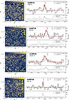 |
Fig. A.3. Continuation of Fig. 4 for G28P1 A and B. |
| In the text | |
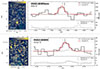 |
Fig. A.4. Continuation of Fig. 4 for IRAS18089 mm and C. |
| In the text | |
|
Fig. A.5. Detection of OH emission in IRAS23385 A. We include a single-component Gaussian fit to the central line, which is a narrow blend of the two central lines in each OH quartet. |
| In the text | |
|
Fig. A.6. Continuation of Figure 3. Full MIRI spectrum of the labeled protostars (black). It shows several absorption features, where the broader one at 9.7 μm is produced by silicate grains. Two blackbody components absorbed by silicates and H2O are fitted to reproduce the overall continuum. The blue curve represents the fit obtained by considering those spectral ranges that are predominantly absorbed by silicates and H2O (in red, also indicated by the R1-R4 anchor ranges in top panel). The green curve shows the modeled blackbody emission only absorbed by silicates, while the dotted magenta curve shows the modeled blackbody emission unaffected by absorption. The black dashed curve above the main silicate absorption feature at 9.7 μm is an interpolation of the silicate-absorbed continuum from a polynomial fit. Here, the red vertical line highlights the resulting depth of the feature that determines τ9.7, whose uncertainty is given by the other two polynomial fits passing above and below (grey curves). The black dashed line at R4 indicates the location of the secondary silicate absorption feature. |
| In the text | |
|
Fig. A.7. Continuation of Figure 3. For IRAS18089 A and C we masked the very deep absorption features at 5.9 and 6.9 μm as it shows mostly noise. |
| In the text | |
|
Fig. B.1. Examples of continuum subtraction on two adjacent, high-flux pixels at the IR source A of IRAS18089 that show contrasting behaviors. The pixel spectrum of the left panel displays the Humphreys alpha line, while the spectrum on the right panel shows a deep artifact that we masked prior to the fitting (red line). In this case the artifact consists of two contiguous, negative channels, where the deeper one is capable of deviating the polynomial fit significantly. The shaded area highlights the spectral range that was excluded when fitting the continuum. The left panel is, at the same time, a good representation of how the continuum subtraction works for the remaining five regions as they do not show negative artifacts. The vertical lines show the nominal wavelength of the Hu α line. |
| In the text | |
Current usage metrics show cumulative count of Article Views (full-text article views including HTML views, PDF and ePub downloads, according to the available data) and Abstracts Views on Vision4Press platform.
Data correspond to usage on the plateform after 2015. The current usage metrics is available 48-96 hours after online publication and is updated daily on week days.
Initial download of the metrics may take a while.