| Issue |
A&A
Volume 709, May 2026
|
|
|---|---|---|
| Article Number | A21 | |
| Number of page(s) | 19 | |
| Section | Catalogs and data | |
| DOI | https://doi.org/10.1051/0004-6361/202558260 | |
| Published online | 28 April 2026 | |
Morphologies for DECaLS galaxies through a combination of nonparametric indices and machine learning methods
A comprehensive catalog using the Galaxy Morphology Extractor (galmex) code
1
Instituto de Física, Universidad Técnica Federico Santa María,
Av. España 1680,
Valparaíso,
Chile
2
Millennium Nucleus for Galaxies (MINGAL),
Chile
3
Departamento de Astronomía, Universidad de La Serena,
Avda. Raúl Bitrán 1305,
La Serena,
Chile
4
Departamento de Astronomía, Facultad Ciencias Físicas y Matemáticas, Universidad de Concepción,
Av. Esteban Iturra s/n Barrio Universitario, Casilla 160,
Concepción,
Chile
★ Corresponding author: This email address is being protected from spambots. You need JavaScript enabled to view it.
Received:
25
November
2025
Accepted:
26
February
2026
Abstract
Context. Galaxy morphology encodes key information about formation and evolution. Large imaging surveys require automated, reproducible methods beyond visual inspection. Nonparametric indices provide a useful framework, but their performance must be quantitatively assessed.
Aims. We present a homogeneous catalog of nonparametric morphological indices for DECaLS galaxies with effective radii larger than 2 arcsec. Our goal is to evaluate the reliability of indices in separating spirals and ellipticals, test their consistency with existing classification schemes, and establish their applicability for the upcoming surveys focused on the southern hemisphere.
Methods. We developed galmex, a modular Python package for preprocessing images and measuring a variety of nonparametric indices. Using bona fide spirals and ellipticals as control samples, we assessed the discriminatory power of each index, and compared them with CNN-based T-Types and Galaxy Zoo DECaLS labels. We used the indices as input for a light gradient boosting machine (LightGBM) to obtain probabilistic classifications.
Results. Concentration is the most reliable parameter from the concentration and asymmetry and smoothness system (CAS), while asymmetry-based indices (A and S) are limited to detecting disturbed morphologies. MEGG indices (M20, Entropy, Gini, G2) provide stronger separation and trace a gradient with T-Type. By using a simple binary (0 or 1) label for ellipticals and spirals, classifiers trained on nonparametric indices achieve high accuracy and well-calibrated probabilities, dominated by entropy, concentration, and Gini. Conclusions. We release the first public catalog of CA[As]S+MEGG indices for DECaLS, together with galmex. We combine the nonparametric indices with machine learning framework to derive spiral and elliptical separation for galaxies below z ~ 0.15 through a probabilistic approach.
Key words: galaxies: elliptical and lenticular, cD / galaxies: general / galaxies: spiral / galaxies: structure
© The Authors 2026
 Open Access article, published by EDP Sciences, under the terms of the Creative Commons Attribution License (https://creativecommons.org/licenses/by/4.0), which permits unrestricted use, distribution, and reproduction in any medium, provided the original work is properly cited.
This article is published in open access under the Subscribe to Open model. This email address is being protected from spambots. You need JavaScript enabled to view it. to support open access publication.
1 Introduction
Early galaxy classification schemes (e.g., Hubble 1926) established the distinction between ellipticals, spirals, and lenticulars, emphasizing that structural appearance is not merely descriptive but encodes a galaxy’s formation and evolutionary history. During formation, the angular momentum of progenitor molecular clouds plays a decisive role in determining the initial morphology of galaxies. Systems with a high specific angular momentum preferentially settle into rotationally supported disks, while low-angular-momentum clouds are more prone to collapsing into spheroid-dominated structures (e.g., Peebles 1969; Teklu et al. 2015). However, morphology is not static. Over cosmic time, both internal processes and environmental interactions can restructure galaxies, altering their stellar distributions, kinematics, and star formation activity. These transformations can be gradual - through secular processes - or rapid, driven by violent interactions or gas removal events (e.g., Toomre & Toomre 1972; Barnes & Hernquist 1991; Kormendy & Kennicutt 2004; Wetzel et al. 2013).
It is now well known that morphology reflects the interplay between internal and environmental mechanisms. Internal drivers include bar-driven secular evolution (Kormendy & Kennicutt 2004; Sanchez-Janssen & Gadotti 2013), disk instabilities (Dekel et al. 2009; Bournaud 2016), and stellar or active galactic nucleus feedback (Dalla Vecchia & Schaye 2008; Fabian 2012), which can redistribute angular momentum, trigger or quench star formation, and alter bulge-to-disk ratios. Environmental processes are particularly relevant in dense regions of the cosmic web, where galaxy-galaxy interactions, harassment, and ram-pressure stripping can significantly reshape systems (Gunn & Gott 1972; Larson et al. 1980; Abadi et al. 1999; Johnston et al. 1999; Balogh et al. 2000; Springel & Hernquist 2005). The morphology-density relation (Dressler 1980; Dressler et al. 1997) encapsulates these environmental trends, and drastic environmental-driven morphological transitions are observed, as in “jellyfish” galaxies for example (Poggianti et al. 2017; Jaffé et al. 2018; Bellhouse et al. 2019).
The cumulative effects of these mechanisms suggest a broad evolutionary pathway in which many galaxies migrate from star-forming, disk-dominated systems to quiescent, spheroidal ones. However, the build of this bimodality and the connection between star formation and morphology can depend on redshift. In the local Universe, star-forming spirals populate the “blue cloud,” while quiescent ellipticals dominate the “red sequence,” with transitional systems lying in the “green valley” (Strateva et al. 2001; Baldry et al. 2004; Schawinski et al. 2014). Toward higher redshift, z ~ 2 star-forming galaxies have clumpy morphologies (Förster Schreiber et al. 2011), with galactic winds that are mainly driven by outflows from prominent star-forming clumps (Genzel et al. 2011) and have not yet formed a stable disc (or any disc at all). On the other hand there is observational evidence of the relation between colour and morphology at high redshift (e.g., Cassata et al. 2005) and a suggestion of disk galaxies at very high redshifts (e.g., Ferreira et al. 2022). This highlights how the investigation of galaxy structural transformation is complex, with the signatures of the underlying mechanisms sometimes being subtle and hard to disentangle observationally.
Despite its importance, there is no universal method to classify galaxy morphology. Visual classification remains intuitive and effective at low redshift (Sandage & Tammann 1987; Sandage & Bedke 1994; Nair & Abraham 2010), but is limited by subjectivity (especially at higher redshifts) and applicability to very large samples. Parametric approaches, such as Sér-sic profile fitting (Sérsic 1963; Sersic 1968; Peng et al. 2002; Simard et al. 2002; Peng et al. 2010; Simard et al. 2011), although simple in form, are not directly applicable to all types of galaxies due to assumed symmetries. Degeneracies between fit parameters (e.g., bulge-to-disk ratios, effective radii, Sérsic index) often produce multiple statistically acceptable but physically distinct solutions (Lotz et al. 2004). Substructures such as compact nuclei, bars, or spiral arms can further bias fits, while even bulges themselves are not uniformly well described by high Sérsic indices (Carollo 1999). Finally, these methods assume that galaxies follow smooth, symmetric light profiles, an assumption that breaks down in irregular, clumpy, or merging systems, yielding degenerate structural parameters (Andrae et al. 2011). Nonparametric indices - including concentration, asymmetry, and smoothness (CAS; Conselice 2003) - provide a model-independent approach, enabling structural characterization across diverse morphologies. The shape asymmetry (AS, Pawlik et al. 2016) can also be relevant in defining disturbed systems, and thus forming the CA[AS]S system. Beyond the CA[AS]S, the combination of M20 (Lotz et al. 2004), Shannon entropy (E, Ferrari et al. 2015), the Gini index (G Lotz et al. 2004), and gradient pattern asymmetry (G2 Rosa et al. 2018) - the MEGG system - has demonstrated an improved performance in separating early- and late-type galaxies in the z ≤ 0.1 Universe (Kolesnikov et al. 2024). Still, the measurement of nonparametric indices is heavily dependent on image preprocessing steps (e.g., object detection, cleaning, and segmentation mask). More recently, machine- and deep-learning methods now enable the automated classification of millions of galaxies (e.g., Barchi et al. 2020; Walmsley et al. 2022), though their interpretability depends strongly on the adopted training sets and classification schema, necessitating extra caution.
In this first paper, we provide a homogeneous, publicly available catalog of nonparametric morphological indices for all galaxies below z ≤ 0.15 in the Dark Energy Camera Legacy Survey (DECaLS, Dey et al. 2019) observed in the r band. The measurements are produced with the newly developed Galaxy Morphology Extractor (galmex) package that, unlike the available codes in the literature, has a modular structure that allows for the fine-tuning of every image preprocessing step, and metric definitions. This structure is particularly suitable for delivering reliable CA[AS]S + MEGG indices with flexible options. Focusing on this catalog, we limit this first paper to the fundamental separation between spirals and ellipticals. Using Galaxy Zoo classifications as training labels, we employ a light gradient boosting machine (LightGBM) to derive probabilistic classifications for all galaxies in DECaLS, calibrated directly in the nonparametric parameter space. The treatment of disturbed systems - including mergers, tidally perturbed, and ram-pressure-stripped galaxies - will be presented in a forthcoming work (Sampaio et al. in prep), as will the extension of this method toward higher redshifts (Vélliz Astudillo et al. in prep.).
This paper is organized as follows. Section 2 describes our data selection from DECaLS, the definition of our labeled spiral and elliptical and spiral control samples, and the adopted morphological indicators. Section 3 introduces the galmex package and its preprocessing and measurement procedures. Section 4 evaluates the performance of the indices and their consistency with previous classifications. Section 5 applies these metrics to a LightGBM to derive probabilistic classifications up to z = 0.15. Section 6 summarizes our conclusions. We assume a flat Λ cold dark matter cosmology with [ΩM, ΩΛ, H0] = [0.27,0.73,72, km s−1 Mpc−1] (Planck Collaboration XIII 2016), and report magnitudes in the AB system.
2 Data
To develop our galaxy classification technique, we selected galaxies from DECaLS1, in the r band. The choice of the Legacy sample is motivated by the combination of a large sky footprint, good depth, and multiwavelength coverage achieved by the survey in the southern hemisphere. Additionally, it also has a substantial overlap with upcoming 4MOST spectroscopic surveys - for example, the CHileAN Cluster Evolution Survey (CHANCES; Haines et al. 2023) and the William Herschel Telescope Enhanced Area Velocity Explorer (WEAVE; Jin et al. 2024) - and is thus a fundamental and reliable morphological classification of systems in the southern hemisphere.
Given that LS-DR10 reaches a median 5σ depth of 23.5 in the r band, with nearly uniform image quality across the footprint, we imposed a bright magnitude limit of mr ≤ 21. This placed our galaxies more than 2 magnitudes above the nominal survey depth, ensuring a high signal-to-noise ratio (S/N) per pixel in both the central regions and the outskirts. Furthermore, nonparametric indices are intrinsically pixel-based measurements, and their reliability deteriorates rapidly as the number of galaxy pixels decreases. Thus, by requiring an effective radius2 greater than 2 arcsec we minimized the biases and increased scatter that arise when these indices are estimated for barely resolved, undersampled systems. Finally, to avoid galaxies dominated by the effect of the point spread function (PSF), which can also deeply influence the nonparametric indices estimation (Walmsley et al. 2022), we only selected galaxies with K ≥ 20, where K is defined as
 (1)
(1)
where Re and FWHM are the effective radius and the point spread function full width at half maximum (∼1.3 arcsec for DECam in the r band), respectively. This results in an initial sample of 6 716 178 galaxies.
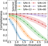 |
Fig. 1 Detection completeness as a function of the SEXTRACTOR detection threshold, k (in units of the background rms), for simulated Sérsic galaxies at different S/N. Solid lines show the median completeness across 1000 realizations per S/N; shaded bands indicate the 1σ scatter. The vertical dashed line marks our adopted threshold k = 1, which maintains ≳70% completeness for S/N ≥ 8 while limiting spurious detections. |
2.1 Observational limits of DECam
To investigate the completeness and the limiting surface brightness that we provide reliable classifications, we carried out controlled simulations of galaxies modeled with Sérsic profiles spanning a wide range of Sérsic indices (n), ellipticities, position angles, and redshifts. We first quantified how detection completeness depends on the SEXTRACTOR detection threshold. For each S/N ∈ {5, 8, 12, 20, 40, 80} we simulated 1000 Sérsic galaxies with parameters drawn uniformly from 1 ≤ n ≤ 5, 1 ≤ Reff ≤ 10 arcsec, axis ratio 0.3 ≤ q ≤ 1, and position angle 0° ≤ θ ≤ 90°. Completeness was defined as the fraction of input sources recovered by the detection algorithm (SExtractor). As is shown in Fig. 1, increasing the threshold suppresses detections at low S/N, while high-S/N sources remain nearly unaffected. Guided by these curves, we adopted a threshold of k = 1 (in units of the background root mean square (rms)), which preserves a completeness ≳95% for S/N ≥ 20 while limiting spurious detections from background fluctuations. Thus, we removed galaxies with a S/N smaller than 20 from our sample (2%).
Second, we investigated how the combination of detection threshold and object surface brightness can affect both detection completeness and shape parameters estimates (central coordinate - r, eccentricity - e, and position angle - θ). In Fig. 2 we show the variations of such parameters in the mean surface brightness within 2Re ( , in mag arcsec−2) versus the detection threshold. Each cell is colored with the average difference (across different Sérsic indices) between true and measured values. The vertical dashed black line marks the threshold adopted in our pipeline. Furthermore, we also highlight that the main differences between true and measured properties occur for objects with 〈μ2Reff〉 fainter than 26 mag arcsec−2. Therefore, we limited our analysis to objects brighter than 〈μ2Reff〉 = 26 mag arcsec−2, which is highlighted by the horizontal dashed red line, and reduced our sample to 6088 103 galaxies.
2.2 Defining labeled subsamples
Despite providing morphology for all galaxies, the morphological classification using nonparametric indices relies on a labeled dataset to define the separations between different morphological types. In this subsection we describe the definition of spiral and elliptical subsamples, which were used as the basis to derive morphological probabilities for our entire galaxy set.
2.2.1 Visual morphologies from Galaxy Zoo
A natural first step in morphological analysis is the binary classification between spirals and ellipticals. In the context of DECaLS, the Galaxy Zoo-DECaLS (GZ DECaLS, hereon) project (Walmsley et al. 2022) provides large-scale visual classifications. However, the classification scheme adopted in GZ DECaLS classify galaxies is between “smooth” or “diskfeature,” which is not a direct mapping onto “spiral” or “elliptical.” Notably, the separation between smooth and disk-feature is considerably subjective and not necessarily exclusive. For example, a disk-dominated system may be classified as smooth if the disk lacks clear features, while some bulge-dominated galaxies may still receive non-negligible disk-feature votes.
We therefore turn to the original Galaxy Zoo 1 (GZ1, hereafter) project (Lintott et al. 2008), which provides explicit spiral and elliptical classifications for SDSS galaxies. Hereafter, we defined the spiral (simply “Sp” hereon) and elliptical (“Ell” hereafter) subsamples according to the GZ 1 project3, focusing on ones that are also on the DECaLS footprint. Since the difference between SDSS and DECam pixels scales are somewhat small (0.396 vs. 0.261 px, respectively), and they have comparable PSFs in the r band (1.18” for DECaLS vs. 1.32” for SDSS), we do not expect these labels to change between surveys. This is reinforced by Fig. 3, in which we show the distribution of the elliptical and spiral subsamples in the top-level classification scheme of GZ DECaLS. Namely, we define fsmooth (x axis), and fdisk (y axis) as the debiased fraction4 of votes that the object is smooth or a disk-feature, respectively, in the GZ DECaLS. Both the Sp and Ell samples lie well within the anticorrelation line (dashed black line), even though ellipticals show a larger spread, highlighting that these are robust subsamples even though their label has been defined in a different survey.
We used Sp and Ell galaxies as control samples, and also as benchmarks for calibrating nonparametric morphological indices. In this first paper, we focus on providing the morphology for galaxies within the redshift coverage of both GZ 1 and GZ DECaLS5; namely, systems below redshift 0.15. Imposing this redshift cut, we end up with a control sample of 80 516 galaxies6. For completeness, a detailed comparison between GZ1 and GZ DECaLS is presented in Appendix B. In a few words, our analysis shows that differences in the Galaxy Zoo classification schemes can significantly impact the purity of selected samples. The extension of our method to higher redshifts (up to 0.5) and the impact of redshift on the nonparametric indices will be discussed in a future paper (Vélliz Astudillo et al. in prep.). Yet, by artificially redshifting galaxies closer than z < 0.03 to z = 0.15, in steps of 0.03, we find that the metrics do not vary by more than 10%, ensuring consistency across the entire redshift range.
Finally, the redshift limit in the control sample implies that, for consistency, we must limit the galaxies that we classify to the same redshift range. Although spectroscopic redshift is only available for 7% of our sample, we applied this cut using the photometric redshift, which is shown to be consistent with the spec z (see Appendix C). A caveat of adopting the labels from GZ 1 is that it is limited in magnitude to 17.78 in the r band, whereas the DECaLS is able to provide deeper observations. Therefore, we adopted the upcoming CHANCES low-z sub survey conservative magnitude limit of 18.5 (Méndez-Hernández et al. in prep.) for our sample, resulting in a final sample of 1 744 454 galaxies (of which 80 516 are labeled as either spiral or elliptical).
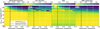 |
Fig. 2 anel a: detection completeness in the 〈μ2Re〉 vs. detection threshold. Panels b-d: average difference between true and measured central position, eccentricity, and position angle, respectively, in the same grid as panel (a). We also highlight two different lines: (1) the dashed black line shows the detection threshold adopted in our pipeline; and (2) the dashed red line shows the conservative threshold in surface brightness, such that we can still recover reliable galaxy properties. |
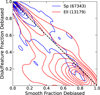 |
Fig. 3 Distribution of GZ 1 selected spiral and elliptical subsamples in the fsmooth versus fdisk (see text for the definition) diagram, according to GZ DECaLS results. The dashed black line shows the expected anticorrelation line. |
2.2.2 Automated classifications from deep learning
Beyond direct visual classifications, we also incorporated automated morphological estimates obtained with convolutional neural networks (CNNs), in order to compare the indices performance both with a visual inspection from GZ DECaLS and as a function of T-Type (Sect. 4.2). To this end, we adopted the catalog of Domínguez Sánchez et al. (2018), which trains CNNs on Galaxy Zoo 2 questions to predict a continuous T-Type for SDSS galaxies, encompassing both our Sp and Ell subsamples. T-Type is estimated as a continuous numerical proxy for the classical Hubble sequence, through the equation
 (2)
(2)
where P(X) denotes the CNN attributed probability of a galaxy being classified as a given morphology, with X representing Elliptical (Ell), lenticular (S0), A-B spiral (Sab), and C-D spiral (Scd). This provides a quantitative mapping onto the classical Hubble sequence, ranging from ellipticals (T-Type ≈ −3) through lenticulars (T-Type ≈ −0) and spirals (T-Type ≈ 15). We highlight that we do not use the T-Type as a label in any step of our method, being included in the catalog only for connecting nonparametric indices to previous machine-learning classifications of galaxy morphology.
3 Nonparametric morphological estimation
We chose a nonparametric method to characterize the structure of galaxies, given that they do not rely on any assumption about the light profile of the observed galaxies, have a direct physical interpretation, and have been extensive used in the literature to connect structural parameters and galaxy evolution related mechanisms (Abraham et al. 1996; Conselice et al. 2000; Lotz et al. 2008; Conselice et al. 2008). However, a fundamental step when measuring nonparametric indices is the need for image preprocessing. Here we present our own Python package (Sect. 3.1) to perform image processing and metrics measurements. The choice of creating our own code is to ensure transparency and the need for fine-tuning, which is not found in non-modular existing codes with the same purpose (e.g., Ferrari et al. 2015; Rodriguez-Gomez et al. 2019).
3.1 The galmex package
The Galaxy Morphology Extractor7 (galmex) is a user-friendly Python package designed to reliably estimate nonparametric morphological indices from imaging surveys. The code is designed with a modular architecture, allowing each stage (preprocessing, segmentation, measurement, output) to be accessed independently. Users can therefore customize the workflow, integrate new routines, or apply only a subset of the available tools. In addition to a command-line interface (CLI) optimized for large-scale processing, galmex also includes a graphical user interface (GUI) for more interactive analysis and visualization. This design makes the package suitable both for bulk catalog production and for detailed inspection of individual galaxies. Next we detail the preprocessing steps adopted prior to measuring the indices:
Cutout creation - For each target we read the right ascension, declination, and a prior Petrosian angular scale from the input catalog, and then requested the stamp in the r band from the Legacy Survey (DR10) cutout service. The linear size of the cutout in pixels was set as the reported effective radius multiplied by a factor of 20 (10 effective radius around the galaxy):
Background subtraction - we estimated and removed the sky using a frame-based statistic around the image edges, since our cutouts are made with size given as a function of the effective radius of the galaxy (10 × Reff). Specifically, we selected a border containing a fixed fraction of the image area and computed background statistics on those pixels with sigma-clipping enabled to suppress contamination from secondary sources near the image border. In practice we set the frame width by an image-area fraction of 0.2, enabled sigma-clipping, and rejected pixels above a 2.5σ threshold; the resulting background model was subtracted from the science image to produce a background-subtracted frame for all subsequent steps;
Object detection - sources were identified on the background-subtracted image with the analog of Source Extractor (Bertin & Arnouts 1996), transcribed to Python - SEP (SExtractor-in-Python, Barbary et al. 2016) - using a matched-filter option. We adopted a per-pixel detection threshold of 1.0σ relative to the measured background noise, required a minimum footprint of ten connected pixels, and deblended with 32 thresholds at a contrast parameter of 0.005; we passed the measured background standard deviation to SEP so that its internal thresholding was on the correct noise scale. SEP returned a normalized catalog (centroid x, y; ellipse a, b; position angle, θ (in radians); npix; mag) and a first segmentation map. The primary galaxy was selected as the label at the cutout center; if the center falls on background, an error was raised, highlighting that no object was detected at the image center.
Cleaning (removal of secondaries) - to mitigate contamination from stars and neighboring galaxies, we generated a cleaned image using an isophotal “painting” procedure that respects the target’s geometry. Starting from the detection segmentation, all labels other than the main object are treated as contaminants; their pixels are replaced via elliptical-isophote interpolation oriented by the galaxy’s position angle, θ. Operationally, the algorithm scans concentric elliptical annuli and replaces masked pixels with interpolated values from adjacent pixels along the same isophote, which preserves the target’s radial structure while suppressing flux from secondaries. This yields a “galaxy-only” image used for all light-profile quantities that follow;
Characteristic radii estimation - we computed Petrosian profiles on the cleaned image using both circular and elliptical annuli, anchored to the SEP-measured center (x,y), axes (a, b), and position angle, θ. The Petrosian radius (RP) follows the standard η(R) = 0.2 threshold with an optimized search: a guided (bisection-style) evaluation of the curve that uses cubic interpolation and takes into account neighboring points (crossing point ± 3). After RP was determined, we derived the circular and elliptical half-light radii by integrating the growth curve to the 50% level, restricting the search to 2 × RP, with a 1-pixel step. We also reported a Kron-style radius computed within the same outer bound. This procedure was executed twice - first with circular annuli and then with elliptical annuli - so that different analyses could use the most appropriate geometry.
An example of the preprocessing procedure is shown in Appendix E.
3.2 Robustness of galmex applied to DECam images
In this section, we test how well galmex recovers galaxy properties using the DECam-like simulated Sérsic profiles described in Sect. 2.1. In particular we focus on the radii encompassing 20, 50, and 80% of the total flux, due to its tracing of the growth curve and direct relation to the concentration index, and the Petrosian radius8, which is extensively used in the literature to define the segmentation mask - i.e., the region that will be taken into account in metrics computation. In Fig. 4, we show the average difference between the true and measured R20 (panel a), R50 (panel b), R80 (panel c), and RP (panel d), in the apparent magnitude versus effective radius grid. For these computations, we used elliptical apertures. We discuss in Appendix F how the use of circular apertures to calculate characteristic radii can introduce significant bias in the analysis. Notably, the combination of apparent magnitude and effective radius defines an average surface brightness9, which is shown by the dashed red lines. The hatched red region denotes the region fainter than our adopted limit in average surface brightness (26 mag arcsec−2). Noteworthy, this is the region where we find the larger offsets (particularly in panel d), again reinforcing that our adopted thresholds ensure that we are providing reliable metrics for all the objects. In particular, Fig. 4 reveals that we recover the characteristic radii with average differences smaller than 0.6 arcsec in most of the cases, which corresponds to a difference of 2.3 pixels in the DECam resolution (∼0.262 pixels/arcsec).
Finally, a key step in the computation of nonparametric indices is the definition of the segmentation mask. To ensure consistency across galaxies of different magnitudes and redshifts, we compared the mean pixel intensity in the r band as a function of radius, written as a function of the Petrosian radius (k × Rp). By scaling the mask with Rp, we guarantee a relative aperture size that adapts to the galaxy’s intrinsic light profile, providing a homogeneous basis for comparison. Following Kolesnikov et al. (2024); Lotz et al. (2004), we defined the conservative threshold of k = 1. We highlight that, unlike statmorph, we used the same segmentation mask for all the metrics, which also ensured a more direct interpretability of their performance in separating ellipticals and spirals. For completeness, we show in Appendix G how segmentation affects our results, in particular on how segmentation affect the separation between spirals and ellipticals in the nonparametric indices diagrams.
 |
Fig. 4 Recovery of characteristic radii across size-flux space. Each panel shows the map of the average absolute difference (in arcsec) between the measured and reference values of a given radius - R20 (a), R50 (b), R80 (c), RP (d) in the apparent magnitude vs. Re. The dashed red lines define the approximate average surface brightness when assuming a circular (q = 1) Sérsic profile. The hatched region above the 〈μ2Re〉 denotes the adopted threshold in this work. Galaxies with a surface brightness smaller than 26 mag s−2 can yield unreliable shape parameters and characteristic radii. In particular, the hatched region overlaps significantly with the region in which the error in RP exceeds 1 arcsec (∼4 pixels). This effect is more visible in RP due to it having the outermost radii in comparison to the others, and thus being more prone to background contamination. |
4 Results
4.1 Nonparametric morphological properties of galaxies
Figure 5 shows the one- and two-dimensional distributions of spiral and elliptical control samples across the CAS and MEGG parameter spaces. The contours highlight the normalized density distributions for each class (15, 25, 50, 60, 70, 80, 90, and 95%), enabling a quantitative comparison of their separation. Overall, the C[AS]AS parameters retain their classical behavior. Concentration shows the strongest discriminatory power, with ellipticals occupying systematically higher values than spirals, consistent with their centrally concentrated light profiles. Asymmetry (A and AS) and smoothness are more effective at rejecting extreme outliers (e.g., mergers), but their distributions overlap significantly between spirals and ellipticals, limiting their power as stand-alone classifiers. This behavior has been reported in previous works (e.g., Kolesnikov et al. 2024), and is confirmed here with the larger DECaLS samples.
The MEGG parameters provide complementary information. The Gini index and entropy exhibit clear trends, with ellipticals clustering at high G and low E, while spirals show the opposite behavior. The M20 parameter retains sensitivity to bright off-center regions, helping to separate star-forming disks from smooth spheroids, although with substantial overlap. The E index stands out as the most effective single discriminator: spirals and ellipticals are distributed with minimal overlap. This corroborates previous results that the MEGG system provides robust morphological separation in both local and intermediateredshift samples (Barchi et al. 2020; Kolesnikov et al. 2024, 2025).
To move beyond a purely visual comparison, we quantified the degree of overlap between the spiral and elliptical distributions using the overlap coefficient (OVL). For a single index X, we computed normalized histograms on shared bin edges for each class and defined the 1D overlap as
![Mathematical equation: \mathrm{OVL}_{\mathrm{1D}}(X) = \sum_{k=1}^{K} \min \big[ p_k(X),\, q_k(X) \big],](/articles/aa/full_html/2026/05/aa58260-25/aa58260-25-eq4.png) (3)
(3)
where pk and qk are the spiral and elliptical probabilities in bin k. Values close to unity indicate nearly indistinguishable distributions, while values near zero indicate strong separation. For a indices-pair (X, Y), we applied an empirical probability-integral transform to each axis, mapping both classes onto the unit square (0,1)2, and then computed a two-dimensional histogram intersection,
![Mathematical equation: \mathrm{OVL}_{\mathrm{2D}}(X,Y) = \sum_{i,j} \min \big[ P_{ij}(U,V),\, Q_{ij}(U,V) \big],](/articles/aa/full_html/2026/05/aa58260-25/aa58260-25-eq5.png) (4)
(4)
with Pij and Qij being the spiral and elliptical probabilities in bin (i, j). This normalization ensures that OVL values are comparable across different index pairs.
Quantitatively, the most effective single indices are concentration, entropy, and Gini, with OVLID ≃ 0.18-0.21, followed by M20 and G2 with OVLID ≃ 0.26-0.27. Asymmetry, shape asymmetry, and smoothness show substantially larger overlaps (≳0.5), confirming that they are better suited to identifying disturbed morphologies than to separating spirals from ellipticals. Of all the 2D projections, the best separation is found for the involving the Gini index, showcasing that this flux-inequality measure is reliable when separating late- and early-type galaxies.
While empirical linear divisions in each 2D plane to separate spiral and elliptical thresholds can be drawn, the overlap between the distributions, particularly in A, AS, and S, suggests that no single cut provides a reliable classification. Instead, the joint use of CA[AS]S+MEGG indices in a probabilistic framework (Sect. 5) provides a more robust approach to assigning morphological classes. In summary, the CA[AS]S parameters reproduce the expected trends but with considerable overlap, while the MEGG indices - especially E and G - deliver superior discriminatory power.
4.2 Comparison to previous classifications
In this subsection, we compare the CA[As]S+MEGG indices with two independent morphological classification schemes in order to place them on a common scale and test their consistency. First, we investigate their variation as a function of the CNNbased T-Type from Domínguez Sánchez et al. (2018). This allows us to assess whether the indices trace the expected early-to-late morphological sequence in a monotonic way. Second, we examine how the same indices vary across the GZ-DECaLS top-level separation (fsmooth vs. fdisk).
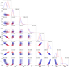 |
Fig. 5 Distribution of spiral (blue curves) and elliptical (red curve) galaxies in 2D diagrams combing the different nonparametric indices. In each panel, we also include the overlap between the spiral and elliptical distributions, which was calculated using Eqs. (3) and (4) for histograms and 2D diagrams, respectively. |
4.2.1 C[AS]AS+MEGG versus CNN-based T-Type
Figure 6 shows the median values and 1σ scatter of the C[AS]AS and MEGG indices as a function of CNN-based T-Type. For robustness, medians and scatters were computed only for T-Type bins containing at least 1% of the corresponding control subsample (Sp or Ell). As a first check, we confirm that the GZ 1 control samples are fully consistent with this scheme: spiral galaxies lie dominantly at T-Type > 0, while ellipticals occupy T-Type < 0.
The CAS indices show the expected broad separation between early- and late-type morphologies. Concentration shows a discontinuity separation between early- and late-type morphologies, varying from 〈C〉 ~ 4.0 at T-Type = −3 to ∼3.0 at T-Type = 5, clearly distinguishing Ell from Sp. This discontinuity may indicate that the T-Type is not as continuous as expected, which may follow from one or a combination of the following reasons: (1) Domínguez Sánchez et al. (2018) use different CNN models for the T-Type ∼ 0 region; (2) the T-Type estimation carries bias from the training dataset; and (3) the equation used to map T-Type continuously is somewhat arbitrary and does not necessarily reflect the continuous transition expected from negative to positive T-Type values. In contrast, A, AS, and S remain nearly constant across T-Type < 0, but increase slightly toward later types. Their variation is modest (∆A, ∆AS, ∆S ≲ 0.08), consistent with their limited discriminatory power for separating Sp from Ell.
The MEGG indices exhibit both clear early-late separation and strong internal trends within the spiral sequence. M20 increases from 〈M20〉 ≃ −2.3 at T-Type = −3 to - − 1.8 at T-Type = 5, possibly due to the increasing prominence of bright off-center regions in late-type spirals. E and Gini display steep, opposite variations: ellipticals cluster at high Gini (≳0.6) and low entropy (≲0.6), while spirals reach 〈G〉 ≃ 0.45 and 〈E〉 ≃ 0.8 at T-Type ∼ 5. The G2 index provides the sharpest discrimination: it remains near zero for ellipticals, increases steadily through early spirals, and reaches 〈G2〉 ≳ 0.45 for the latest types. This steep gradient at T-Type > 0 demonstrates that M20, E, and G not only separates ellipticals from spirals (with a confidence of more than 3 sigma), but also effectively resolves substructure within the spiral sequence.
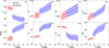 |
Fig. 6 Metrics variations with respect to CNN-based T-Type for the Sp (blue) and Ell (red) subsamples. We highlight that, although both the Sp and Ell classification, and T-Type are based on SDSS data (Galaxy Zoo 1 and 2, respectively), our results show consistency even when using DECam observations. |
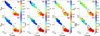 |
Fig. 7 Metrics variation in the smooth debiased vs. disk-feature debiased diagram. In this case we merge the spiral and elliptical subsamples in order to get a full picture of the metrics variation across this diagram. |
4.2.2 Nonparametric indices versus visual classification
Figure 7 presents the variation in C[AS]AS and MEGG indices across the GZ-DECaLS fdisk versus fsmooth plane. Particularly for Fig. 7, we merged the spiral and elliptical subsamples rather than analyzing them separately, in order to provide a complete view of the parameters variation. We restricted the hexbin maps to bins containing at least ten galaxies, and we scaled the color bars in a consistent way such that regions dominated by ellipticals appear in redder tones.
Overall, the indices vary across this diagram in good agreement with the Galaxy Zoo classifications. Concentration, C, increases steadily toward the smooth-dominated corner, while E decreases and Gini increases, reproducing the contrast between bulge-dominated and disk-dominated systems. A, AS, and S peak in the high fdisk regime, consistent with the visual impression of clumpier and more irregular morphologies. M20 also increases in this region, reflecting the prominence of bright off-center structures in spiral galaxies. Finally, G2 shows a marked gradient from smooth to disk-dominated systems, again underscoring its effectiveness as a discriminator.
These trends demonstrate that nonparametric indices are broadly consistent with human visual assessments from Galaxy Zoo, capturing the same underlying morphological differences directly from the pixel data. In other words, CA[AS]S+MEGG indices to some extent mimic what classifiers perceived by eye.
This motivates the next step of our analysis, in which we employ these indices as input features for a machine-learning framework (Sect. 5) to assign probabilistic classifications across the full DECaLS sample.
5 CA[AS]S + MEGG indices as inputs for machine learning classification
To move beyond qualitative trends and improve the accuracy of separating spirals and ellipticals, we combined the measured nonparametric indices with the visual classifications from GZ 1 to train a supervised machine-learning model. This approach used the discriminatory power of the CA[AS]S + MEGG parameter space, while adopting the decision boundaries from reliable visual labels, and enabling the derivation of probabilistic morphological classifications. By doing so, it transformed the indices from descriptive diagnostics into quantitative predictors, allowing us to assign each galaxy a probability of being spiral or elliptical in a homogeneous way.
5.1 Defining a training set
We used our spiral and elliptical subsamples as training set for the machine learning. We used the GZ1 label (elliptical vs. spiral) as the target y ∈ {0,1}, with spiral as the positive class (1). The combined sample was then divided into the pool (60%), calibration (15%), and test sample (25%). Because spirals largely outnumber ellipticals in our sample, we addressed the class imbalance in two ways. First, all splits preserved the class ratio in the pool, calibration, and test sets. Second, we applied SMOTE10 (the synthetic minority over-sampling technique; Chawla et al. 2011) only within the training sets of the cross-validation and in the training portion of the pool set: synthetic minority examples were generated by interpolating between nearest neighbors of the minority class in the C[AS]AS+MEGG feature space. No over-sampling was applied to calibration or test sets, ensuring unbiased performance estimates and well-calibrated probabilities.
5.2 Results using a light gradient boosting machine
To assess the discriminative power of the full set of nonparametric morphological indices, we employed LightGBM (Ke et al. 2017), a decision-tree-based ensemble algorithm that implements gradient boosting in a highly efficient manner. In contrast to classical classifiers that rely on a linear or logistic boundary in the feature space, gradient boosting iteratively builds an ensemble of weak learners (decision trees), whereby each subsequent tree corrects the residual errors of the previous ensemble. LightGBM improves on standard implementations of gradient boosting by using a leaf-wise tree growth strategy and histogrambased binning of features, allowing for faster training, lower memory usage, and the ability to handle large, imbalanced datasets. These properties make LightGBM particularly suitable for our morphological classification problem, where the input feature space is moderately high-dimensional and the class distribution between spirals and ellipticals is not balanced. Furthermore, the algorithm provides well-calibrated probabilistic outputs and interpretable measures of feature importance, both of which are essential for a robust scientific interpretation.
Figure 8 summarizes the performance of the LightGBM classifier. We detail each panel, from leftmost top row, to rightmost bottom row, in the following:
The ROC curve, which quantifies the trade-off between the true positive rate and the false positive rate for varying classification thresholds. The resulting area under the curve (AUC = 0.995 ± 0.001) indicates near-perfect separability between spiral and elliptical galaxies;
The precision-recall (PR) curve, focusing on the performance for the spiral class. The extremely high average precision ([AP] = 0.999 ± 0.000) further confirms that the classifier maintains excellent purity across the full range of recall values;
The probability calibration curve. This diagnostic compares the raw model outputs (predicted probability of being a spiral) against the empirical fraction of true spirals in corresponding probability bins. If the classifier is perfectly calibrated, points will fall along the one-to-one diagonal; for example, of all galaxies assigned a spiral probability of 70%, about 70% should actually be spirals. The plotted blue points represent the mean observed frequencies in probability bins, with error bars denoting the 95% confidence interval. The close alignment with the diagonal line indicates that the LightGBM predictions are almost perfectly calibrated across the full probability range. In the same panel, we show the Brier score (Brier 1950), which provides a quantitative summary of calibration and refinement. It measures the mean squared error between predicted probabilities and the true binary outcomes, taking values between 0 (perfect) and 1 (worst possible). Our measured Brier score of
 is extremely low, meaning that the probabilities are not only discriminative but also reliable. This complements the ROC and PR curves: a model can achieve high AUC or [AP] while still producing poorly calibrated probabilities, but in this case LightGBM achieves both high discrimination and excellent calibration;
The confusion matrix expressed in row-normalized percentages. LightGBM correctly identifies 98.6% ± 0.3 of spiral galaxies and 87.5% ± 0.6 of ellipticals. Misclassifications are rare, amounting to only ∼1.4 ± 0.3% of spirals classified as ellipticals and ∼12.5 ± 0.9% of ellipticals classified as spirals. The latter can follow from the presence of S0s within the elliptical label in GZ1;
The learning (loss) curves of the LightGBM classifier, showing the binary cross-entropy (log loss) as a function of boosting iterations (trees). We plot loss on the raw training fold (no SMOTE) and on an independent validation fold. The validation curve drops rapidly and then flattens without an upturn, indicating no overfitting. The training curve remains below the validation curve, as was expected from the generalization gap11. The training loss remains strictly above zero because we optimize probabilistic log loss under regularization and early stopping; pushing log loss to zero would require assigning probabilities of exactly 0 or 1 to every training object - a behavior typical of overfitting and inconsistent with the probabilistic approach we adopt;
The distribution of predicted spiral probabilities for the true spiral and elliptical systems in the test sample. The strong bimodality, with spirals peaking near unity and ellipticals near zero, highlights the high confidence of the model predictions. Only a negligible fraction of objects occupy the intermediate regime, reinforcing the robustness of the classification.
The very high performance (AUC ≃ 0.99, AP ≃ 1) largely reflects the fact that our target label is intentionally simple (spiral vs. early-type as defined by GZ1) and that the adopted nonparametric morphology vector is designed to separate these two regimes efficiently. We understand that it would be better to have a good separation between ellipticals, lenticulars, and spirals; however, separating ellipticals and lenticulars is a longstanding problem in the literature, and for the current exercise the labels from GZ1 are the most robust that we can use. To address the concern that the result could be driven by a restricted subset of large, high-S/N systems, we performed a sanity check by measuring ROC performance in bins of apparent size and brightness (Fig. 9). Using out-of-fold calibrated probabilities, the classifier continues to perform well across the full range probed: for RP (arcsec) the AUC varies only mildly from 0.991 ± 0.003 (4-10 arcsec) up to 0.996 ± 0.003 (20-30 arcsec), and as a function of r magnitude it decreases smoothly from 0.994 ± 0.004 (14-15) to 0.977 ± 0.016 (17-18). This controlled degradation toward the faintest bins -where morphology is intrinsically harder due to lower resolution and surface-brightness sensitivity - supports the interpretation that the high global AUC and AP is not an artifact of a single easy regime, but rather that the separation remains robust over most of the parameter space while behaving as expected where the task becomes observationally more challenging.
Moreover, since we feed the LightGBM with eight different indices, it is important also to investigate which are contributing the most to define the desired probability. Thus, we applied SHAP (SHapley Additive exPlanations; Lundberg & Lee 2017) values to the LightGBM model, shown in Fig. 10. Each point in the summary plot corresponds to a galaxy, with its horizontal position encoding the SHAP value (i.e., the marginal contribution of that feature to the probability of being classified as a spiral), and the color denoting the normalized feature value.
Negative SHAP values (to the left) lower the spiral probability, while positive values (to the right) increase it. For instance, galaxies with low G (blue points) tend to shift the classification toward spiral, reflecting the clumpy light distribution of disks. Similarly, high entropy increases the spiral likelihood, while low values support elliptical classifications. Overall, the SHAP values not only corroborate the feature importance ranking but also provide physical interpretability by linking specific morphological traits to the classifier’s decision process.
Yet, we highlight one particular caveat of the adopted procedure. Because GZ1 provides only a binary spiral versus elliptical label for bright SDSS galaxies, the “elliptical” class inevitably contains a non-negligible fraction of lenticular (S0) systems: in single-band imaging, S0s share the smooth, centrally concentrated appearance of ellipticals, yet they are physically disk galaxies, often with weak spiral structure and subtle lenses and bars. This mixing is important for calibration: the model is trained (and isotonic-calibrated) to reproduce GZ1’s operational definition of elliptical, so the resulting P(Sp) should be interpreted as the probability of being spiral versus a mixed early-type (E+S0) class, rather than a pure E versus Sp separation. Not by chance, the accuracy in the confusion matrix for ellipticals is smaller than the one for spirals, as we expect most S0s to be included within the ellipticals subset. Nevertheless, S0s can also be misclassified as disk galaxies, particularly with an edge-on line of sight.
In summary, the LightGBM model is able to provide a high accuracy for spiral probability through the use of structural features of galaxies, quantified through the nonparametric indices. In this regard, the most important sets to define the spiral probability are G, C, and E, each of which shows a great separation between GZ 1 selected spirals and ellipticals. We incorporate the P(spiral) for all the galaxies in our sample in the provided catalog, for which the columns and respective descriptions can be found in Appendix I.
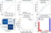 |
Fig. 8 Results of LightGBM using the nonparametric indices as input, and trained in the GZ 1 selected spirals and ellipticals. Panels a and b: ROC curve and the precision-recall curve, respectively. Within these two panels, we also add the area under the curve (AUC) and the mean AP. Panel c: calibration curve, highlighting that our method aligns well with the expected 1 to 1 line, ensuring that our method is able to provide calibrated probabilities. Panel d: row-normalized confusion matrix. Panel e: log-loss function. See the text for a description on why there is a difference between the train and validation. Panel f: predicted spiral probability for galaxies in our test subsample. Notably, our method shows high accuracy. |
 |
Fig. 9 Sanity check of classifier performance as a function of observational regime. Receiver operating characteristic (ROC) curves for the spiral vs. smooth classifier evaluated in bins of (a) apparent size, using the Petrosian radius (arcsec), and (b) r band Petrosian magnitude. Curves show the mean ROC across cross-validation folds, with shaded regions indicating the ±1σ scatter between folds; the corresponding AUC values (mean ± standard deviation) are listed in the legend for each bin. Performance remains high across the full range, with the expected mild degradation toward the smallest, and faintest galaxies where morphology measurements are noisier and resolution is lower. |
 |
Fig. 10 SHapley Additive exPlanations (SHAP) summary plot for the LightGBM model predicting spiral galaxy classification. Each point represents the SHAP value of a single feature for one galaxy, showing its impact on the model output. The horizontal axis indicates the contribution (positive or negative) to the prediction, while the vertical axis lists the most important features ranked by overall impact. The color gradient encodes the feature value from low (blue) to high (red), highlighting how different ranges of feature values drive the prediction toward or away from the spiral class. |
6 Conclusions and summary
In this work we provide the first homogeneous catalog of nonparametric morphological indices for galaxies in the Dark Energy Camera Legacy Survey (DECaLS, part of the Legacy survey, data release 10), limited to systems that have an effective radius larger than 2 arcsec and that are brighter than 18.5 in the r band apparent magnitude. Using our newly developed Python package galmex, we measured the full CA[AS]S+MEGG set of nonparametric indices in a uniform way for more than one million DECaLS galaxies, and derived probabilistic spiral-elliptical classifications for about 1.7 million objects at z ≤ 0.15. The modular, transparent design of galmex ensures that every preprocessing and measurement step can be inspected, reproduced, and adapted, turning the catalog and the code into a long-lived resource for the community.
Compared to previous morphology catalogs based on visual inspection or parametric profile fitting, our work delivers: (i) a deeper and wider-area dataset in the southern hemisphere, fully processed with a single, well-tested pipeline; (ii) a consistent set of C[AS]AS+MEGG indices measured with segmentation and Petrosian apertures tuned on realistic DECam simulations; and (iii) calibrated probabilistic classifications directly in the nonparametric parameter space. This combination provides a more homogeneous and physically interpretable view of galaxy structure than either visual labels alone or purely Sérsic-based decompositions.
Our main conclusions about the reliability and use of nonparametric indices for morphology are:
C[As]AS and MEGG indices - Using bona fide samples of spirals and ellipticals defined from Galaxy Zoo 1, we confirm that concentration is the most reliable CAS parameter for separating early and late types, whereas asymmetry-based indices (A, AS, and S) exhibit substantial overlap between the two classes and are therefore best suited for separating strongly disturbed systems rather than performing a clean spiral-elliptical split (Fig. 5). In contrast, all indices in the MEGG system (M20, entropy, Gini, and G2) provide strong and consistent separation, highlighting their robustness as tracers of bulge- versus disk-dominated morphologies;
Connection with T-Type and visual classification - When compared with CNN-based T-Types (Fig. 6), the indices not only recover the global spiral-elliptical division but also trace a continuous gradient along the Hubble sequence. The trend is particularly steep for M20, E, Gini, and G2, which respond to substructure and clumpiness in spiral galaxies. Moreover, the indices reproduce the distributions obtained from Galaxy Zoo visual classifications (Fig. 7), demonstrating that nonparametric indices capture, to first order, the same morphological traits perceived by human classifiers;
Machine-learning classification - Using their discriminatory power, we provide the indices as input features to a binary LightGBM classifier (Figs. 8 and 10), focused on discriminating between spirals and early-type systems (E+S0s). The model achieves high accuracy (97%) and produces well-calibrated probabilities of a galaxy being spiral, with entropy, concentration, and Gini consistently emerging as the most influential features.
An important caveat that emerges from our analysis is that the reliability of control samples depends strongly on the adopted visual classification scheme. In particular, the top-level separation in Galaxy Zoo DECaLS into smooth versus disk-feature categories is not equivalent to the classical early- versus late-type division. We show that the distributions of nonparametric indices for these DECaLS classes differ significantly from those of ellipticals and spirals selected from Galaxy Zoo 1, with the largest discrepancies appearing when comparing smooth galaxies to elliptical ones. This mismatch reflects the subjectivity of the smooth category, which can include both bulge-dominated disks and genuine ellipticals, and leads to systematically different metric distributions. Moreover, training a machine-learning classifier on the DECaLS smooth-disk labels results in degraded performance compared to using the GZ1 spiral and elliptical subsamples, directly affecting both the reliability and purity of the resulting classifications. These biases are further compounded by the dependence of vote fractions on redshift, luminosity, and Petrosian radius, which imprint observational effects onto the labels themselves. Together, these results highlight that the choice of training set and classification scheme is not a neutral decision: it can propagate systematic biases into automated classifications, underscoring the need for careful sample definition when bridging visual projects and machine-learning frameworks.
In summary, this work establishes a transparent and reproducible framework for morphological classification in wide-field imaging surveys. The combination of a publicly available catalog, a modular software package, and a calibrated machinelearning classifier provides the community with an extremely versatile toolset with which to study galaxy evolution. Because the catalog covers the full DECaLS footprint and overlaps with major spectroscopic programs in the southern hemisphere (e.g., 4MOST-CHANCES and WEAVE), it enables a broad range of new science: from mapping morphology as a function of environment, mass, and star formation activity, to selecting rare disturbed systems, such as mergers and jellyfish galaxies, in a uniform way. The natural next step is to move beyond the simple spiral-elliptical dichotomy and explicitly incorporate disturbed and transitioning systems, as well as to extend the methodology toward higher redshifts. This will allow us to probe more directly the dynamical processes that drive morphological transformation, providing a more complete picture of galaxy evolution across environments and cosmic time.
Data availability
The separated elliptical and spiral catalogs and the full ∼1.7 million galaxies catalog are available at the CDS via https://cdsarc.cds.unistra.fr/viz-bin/cat/J/A+A/709/A21, as well as a readme file. All the codes used to generate results and plots of this paper are available at https://github.com/vitorms99.
Acknowledgements
The acknowledgements are available in Appendix A.
References
- Abadi, M. G., Moore, B., & Bower, R. G. 1999, MNRAS, 308, 947 [Google Scholar]
- Abraham, R. G., Tanvir, N. R., Santiago, B. X., et al. 1996, MNRAS, 279, L47 [Google Scholar]
- Andrae, R., Jahnke, K., & Melchior, P. 2011, MNRAS, 411, 385 [CrossRef] [Google Scholar]
- Astropy Collaboration (Robitaille, T. P., et al.) 2013, A&A, 558, A33 [NASA ADS] [CrossRef] [EDP Sciences] [Google Scholar]
- Astropy Collaboration (Price-Whelan, A. M., et al.) 2018, AJ, 156, 123 [Google Scholar]
- Astropy Collaboration (Price-Whelan, A. M., et al.) 2022, ApJ, 935, 167 [NASA ADS] [CrossRef] [Google Scholar]
- Baldry, I. K., Glazebrook, K., Brinkmann, J., et al. 2004, ApJ, 600, 681 [Google Scholar]
- Balogh, M. L., Navarro, J. F., & Morris, S. L. 2000, ApJ, 540, 113 [Google Scholar]
- Barbary, K., Boone, K., McCully, C., et al. 2016, https://doi.org/10.5281/zenodo.159035 [Google Scholar]
- Barchi, P. H., de Carvalho, R. R., Rosa, R. R., et al. 2020, Astron. Comput., 30, 100334 [NASA ADS] [CrossRef] [Google Scholar]
- Barnes, J. E., & Hernquist, L. E. 1991, ApJ, 370, L65 [Google Scholar]
- Bellhouse, C., Jaffé, Y. L., McGee, S. L., et al. 2019, MNRAS, 485, 1157 [Google Scholar]
- Bershady, M. A., Jangren, A., & Conselice, C. J. 2000, AJ, 119, 2645 [NASA ADS] [CrossRef] [Google Scholar]
- Bertin, E., & Arnouts, S. 1996, A&AS, 117, 393 [Google Scholar]
- Blanton, M. R., Kazin, E., Muna, D., Weaver, B. A., & Price-Whelan, A. 2011, AJ, 142, 31 [NASA ADS] [CrossRef] [Google Scholar]
- Bournaud, F. 2016, in Astrophysics and Space Science Library, 418, Galactic Bulges, eds. E. Laurikainen, R. Peletier, & D. Gadotti, 355 [Google Scholar]
- Brier, G. W. 1950, Monthly Weather Rev., 78, 1 [CrossRef] [Google Scholar]
- Carollo, C. M. 1999, ApJ, 523, 566 [Google Scholar]
- Cassata, P., Cimatti, A., Franceschini, A., et al. 2005, MNRAS, 357, 903 [NASA ADS] [CrossRef] [Google Scholar]
- Chawla, N. V., Bowyer, K. W., Hall, L. O., & Kegelmeyer, W. P. 2011, arXiv e-prints [arXiv:1106.1813] [Google Scholar]
- Conselice, C. J. 2003, ApJS, 147, 1 [NASA ADS] [CrossRef] [Google Scholar]
- Conselice, C. J., Bershady, M. A., & Jangren, A. 2000, ApJ, 529, 886 [NASA ADS] [CrossRef] [Google Scholar]
- Conselice, C. J., Rajgor, S., & Myers, R. 2008, MNRAS, 386, 909 [CrossRef] [Google Scholar]
- Dalla Vecchia, C., & Schaye, J. 2008, MNRAS, 387, 1431 [Google Scholar]
- Dekel, A., Birnboim, Y., Engel, G., et al. 2009, Nature, 457, 451 [Google Scholar]
- Dey, A., Schlegel, D. J., Lang, D., et al. 2019, AJ, 157, 168 [Google Scholar]
- Domínguez Sánchez, H., Huertas-Company, M., Bernardi, M., Tuccillo, D., & Fischer, J. L. 2018, MNRAS, 476, 3661 [Google Scholar]
- Dressler, A. 1980, ApJ, 236, 351 [Google Scholar]
- Dressler, A., Oemler, Augustus, J., Couch, W. J., et al. 1997, ApJ, 490, 577 [NASA ADS] [CrossRef] [Google Scholar]
- Fabian, A. C. 2012, ARA&A, 50, 455 [Google Scholar]
- Ferrari, F., de Carvalho, R. R., & Trevisan, M. 2015, ApJ, 814, 55 [NASA ADS] [CrossRef] [Google Scholar]
- Ferreira, L., Adams, N., Conselice, C. J., et al. 2022, ApJ, 938, L2 [NASA ADS] [CrossRef] [Google Scholar]
- Förster Schreiber, N. M., Shapley, A. E., Erb, D. K., et al. 2011, ApJ, 731, 65 [CrossRef] [Google Scholar]
- Genzel, R., Newman, S., Jones, T., et al. 2011, ApJ, 733, 101 [Google Scholar]
- Gunn, J. E., & Gott, J., Richard, I. 1972, ApJ, 176, 1 [NASA ADS] [CrossRef] [Google Scholar]
- Haines, C., Jaffé, Y., Tejos, N., et al. 2023, The Messenger, 190, 31 [NASA ADS] [Google Scholar]
- Harris, C. R., Millman, K. J., van der Walt, S. J., et al. 2020, Nature, 585, 357 [NASA ADS] [CrossRef] [Google Scholar]
- Hubble, E. P. 1926, ApJ, 64, 321 [Google Scholar]
- Hunter, J. D. 2007, Comput. Sci. Eng., 9, 90 [NASA ADS] [CrossRef] [Google Scholar]
- Jaffé, Y. L., Poggianti, B. M., Moretti, A., et al. 2018, MNRAS, 476, 4753 [Google Scholar]
- Jin, S., Trager, S. C., Dalton, G. B., et al. 2024, MNRAS, 530, 2688 [NASA ADS] [CrossRef] [Google Scholar]
- Johnston, K. V., Sigurdsson, S., & Hernquist, L. 1999, MNRAS, 302, 771 [Google Scholar]
- Ke, G., Meng, Q., Finley, T., et al. 2017, Adv. Neural Inform. Process. Syst., 30 [Google Scholar]
- Kolesnikov, I., Sampaio, V. M., de Carvalho, R. R., et al. 2024, MNRAS, 528, 82 [Google Scholar]
- Kolesnikov, I., Sampaio, V. M., de Carvalho, R. R., & Conselice, C. 2025, MNRAS, 539, 2765 [Google Scholar]
- Kormendy, J., & Kennicutt, Jr., R. C. 2004, ARA&A, 42, 603 [Google Scholar]
- Larson, R. B., Tinsley, B. M., & Caldwell, C. N. 1980, ApJ, 237, 692 [Google Scholar]
- Lintott, C. J., Schawinski, K., Slosar, A., et al. 2008, MNRAS, 389, 1179 [NASA ADS] [CrossRef] [Google Scholar]
- Lotz, J. M., Primack, J., & Madau, P. 2004, AJ, 128, 163 [NASA ADS] [CrossRef] [Google Scholar]
- Lotz, J. M., Davis, M., Faber, S. M., et al. 2008, ApJ, 672, 177 [NASA ADS] [CrossRef] [Google Scholar]
- Lundberg, S. M., & Lee, S.-I. 2017, in Advances in Neural Information Processing Systems, 30, eds. I. Guyon, U. V. Luxburg, S. Bengio, H. Wallach, R. Fergus, S. Vishwanathan, & R. Garnett (Curran Associates, Inc.) [Google Scholar]
- McKinney, W. 2010, in Proceedings of the 9th Python in Science Conference, eds. S. van der Walt, & J. Millman, 56 [Google Scholar]
- Nair, P. B., & Abraham, R. G. 2010, ApJS, 186, 427 [Google Scholar]
- Pawlik, M. M., Wild, V., Walcher, C. J., et al. 2016, MNRAS, 456, 3032 [NASA ADS] [CrossRef] [Google Scholar]
- Peebles, P. J. E. 1969, ApJ, 155, 393 [Google Scholar]
- Peng, C. Y., Ho, L. C., Impey, C. D., & Rix, H.-W. 2002, AJ, 124, 266 [Google Scholar]
- Peng, C. Y., Ho, L. C., Impey, C. D., & Rix, H.-W. 2010, AJ, 139, 2097 [Google Scholar]
- Planck Collaboration XIII. 2016, A&A, 594, A13 [NASA ADS] [CrossRef] [EDP Sciences] [Google Scholar]
- Poggianti, B. M., Moretti, A., Gullieuszik, M., et al. 2017, ApJ, 844, 48 [Google Scholar]
- Reback, J., Jbrockmendel, McKinney, W., et al. 2022, https://doi.org/10.5281/zenodo.3509134 [Google Scholar]
- Rodriguez-Gomez, V., Snyder, G. F., Lotz, J. M., et al. 2019, MNRAS, 483, 4140 [NASA ADS] [CrossRef] [Google Scholar]
- Rosa, R., De Carvalho, R., Sautter, R., et al. 2018, MNRAS, 477, L101 [CrossRef] [Google Scholar]
- Sanchez-Janssen, R., & Gadotti, D. A. 2013, MNRAS, 432, L56 [NASA ADS] [CrossRef] [Google Scholar]
- Sandage, A., & Tammann, G. A. 1987, A Revised Shapley-Ames Catalog of Bright Galaxies [Google Scholar]
- Sandage, A., & Bedke, J. 1994, The Carnegie Atlas of Galaxies, 638 [Google Scholar]
- Schawinski, K., Urry, C. M., Simmons, B. D., et al. 2014, MNRAS, 440, 889 [Google Scholar]
- Sérsic, J. L. 1963, Bol. Asoc. Argentina Astron. Plata Argentina, 6, 41 [Google Scholar]
- Sersic, J. L. 1968, Atlas de Galaxias Australes [Google Scholar]
- Simard, L., Willmer, C. N. A., Vogt, N. P., et al. 2002, ApJS, 142, 1 [NASA ADS] [CrossRef] [Google Scholar]
- Simard, L., Mendel, J. T., Patton, D. R., Ellison, S. L., & McConnachie, A. W. 2011, ApJS, 196, 11 [CrossRef] [Google Scholar]
- Springel, V., & Hernquist, L. 2005, ApJ, 622, L9 [Google Scholar]
- Strateva, I., Ivezic, Z., Knapp, G. R., et al. 2001, AJ, 122, 1861 [CrossRef] [Google Scholar]
- Teklu, A. F., Remus, R.-S., Dolag, K., et al. 2015, ApJ, 812, 29 [Google Scholar]
- Toomre, A., & Toomre, J. 1972, ApJ, 178, 623 [Google Scholar]
- Van Rossum, G., & Drake, F. L. 2009, Python 3 Reference Manual (Scotts Valley, CA: CreateSpace) [Google Scholar]
- Virtanen, P., Gommers, R., Oliphant, T. E., et al. 2020, Nat. Methods, 17, 261 [Google Scholar]
- Walmsley, M., Lintott, C., Géron, T., et al. 2022, MNRAS, 509, 3966 [Google Scholar]
- Wetzel, A. R., Tinker, J. L., Conroy, C., & van den Bosch, F. C. 2013, MNRAS, 432, 336 [Google Scholar]
Data products were retrieved from Legacy Surveys Data Release 10, available at https://www.legacysurvey.org
The effective radius is provided by the Legacy Survey database in the column shape_r.
The GZ 1 project provides a direct classification of spirals and ellipticals, avoiding the need to adopt a threshold in the vote fraction.
In practice, galaxies are binned by absolute magnitude and physical size; within each bin and for each answer (“smooth” or “features-disk”), the vote-fraction distributions at each redshift are shifted to match those of the lowest-redshift slice (0.02 < z < 0.03), yielding the fraction expected if every galaxy were observed at z ~ 0.02 and keeping the fraction above any chosen threshold constant with redshift.
In the original GZ DECaLS catalog, z is the spectroscopic redshift retrieved from the Nasa-Sloan Atlas catalog (NSAtlas Blanton et al. 2011).
Although the number of spiral galaxies is about six times that of ellipticals (13 179 Ell and 67 343 Sp), we explain how we address this imbalance in Sect. 5.1
A full tutorial and description are available in “read the docs” or github.
Notably, galmex relies only on the shape properties estimated during object detection step to reliably calculate the Petrosian radius, whereas statmorph (Rodriguez-Gomez et al. 2019) estimates may depend also on the segmentation mask used as an input.
The surface brightness depends on the eccentricity of the object, but we adopted a simple case of circular Sérsic profile (q = 1).
SMOTE generates synthetic samples through nearest-neighbor interpolation in the minority class feature space, which helps avoid the overfitting associated with simple duplication. Nonetheless, as with any resampling technique, it can introduce bias if classes are highly overlapping in the full space. Since (most) of the metrics show very clear distinction between Ell and Sp (Fig. 5), it is a safe procedure. We also computed the results without using the SMOTE, for which we find similar results. Namely, the overall accuracy decreases by 0.5%, which follows from a decrease in the accuracy specifically for Ell (also small 2%), while the spirals remain “untouched”.
In supervised learning the loss evaluated on the data used for fitting is systematically lower than the loss on unseen data. This difference is the generalization gap. A nonzero separation between train and validation curves is therefore expected and, within bounds, evidence of a model that fits the data while still generalizing.
Appendix A Acknowledgements
We thank the referee for the suggestions that helped improving this paper. This research made use of the Python programming language (Van Rossum & Drake 2009) and the packages NumPy (Harris et al. 2020), SciPy (Virtanen et al. 2020), Astropy (Astropy Collaboration 2013, 2018, 2022), pandas (McKinney 2010; Reback et al. 2022), and Matplotlib (Hunter 2007). This work has been supported by the Agencia Nacional de Investigación y Desarrollo (ANID) through the Millennium Science Initiative Program NCN2024_112 (VMS, YLJ, HME); the BASAL project FB210003 (YLJ, HME, AM); the FONDECYT Regular projects 1241426 and 1230441 (YLJ) and 1251882 (AM); and the FONDECYT project 3250511 (CLD). VMS acknowledges additional support from ESO through grant ORP026/2021, and CLD from the ESO Comité Mixto through grant ORP037/2022. AM further acknowledges funding from the HORIZON-MSCA-2021-SE-01 Research and Innovation Programme under the Marie Sklodowska-Curie grant agreement No. 101086388. VMS thanks RRdC and IK for the fruitful discussions.
Appendix B Comparison of Galaxy Zoo 1 and Galaxy Zoo DECALS
In this appendix we present a comparison between the Galaxy Zoo 1 and Galaxy Zoo DECaLS. In Fig. B.1 we show the variation of fsmooth for ellipticals, and fdisk for spirals, as a function of redshift, absolute magnitude in the r band and Petrosian radius. First, fsmooth is always smaller than fdisk. Irrespective of considered panel, the Galaxy Zoo 1 ellipticals is classified as "smooth" by roughly 70% of the voters. This may indicate a direct influence of the adopted scheme in Galaxy Zoo DECaLS, in which the top-level question ("smooth" or "disk-feature") is considerably subjective, and the concept of an "smooth" is somewhat vague. Thus, even in elliptical galaxies (according to Galaxy Zoo 1), the vote fraction does not reach high percentages (≥ 80%). This has relevant implications to CNN models that use the Galaxy Zoo DECaLS as training samples.
To investigate the variations in the metrics when using subsamples selected directly from the Galaxy Zoo DECaLS, we select galaxies "smooth" and "disk-feature" subsamples as it follows:
Smooth: (fsmooth ≥ 0.7) and (fdisk ≤ 0.3);
Disk-Feature: (fsmooth ≤ 0.3) and (fdisk ≥ 0.7).
In Fig. B.2 we show the CA[AS]S+MEGG distributions for the "smooth" and "disk-feature" samples (dashed lines), besides the Galaxy Zoo 1 Spiral and Elliptical samples (solid lines). Quantitatively, we compare the smooth with the elliptical, and the disk-feature with the disk distributions using the energy distance parameter. The energy distance between two probability distributions P and Q is defined as
![Mathematical equation: D_E(P,Q) \;=\; 2\,\mathbb{E}\bigl[|| X - Y || \bigr] \;-\; \mathbb{E}\bigl[|| X - X' || \bigr] \;-\; \mathbb{E}\bigl[|| Y - Y' || \bigr],](/articles/aa/full_html/2026/05/aa58260-25/aa58260-25-eq7.png) (B.1)
(B.1)
where X, X′ ∼ P and Y, Y′ ∼ Q are independent random variables, and E denotes the expectation of each comparison. This metric is non-negative and equals zero if and only if P = Q, making it a useful tool for quantifying differences. Notably, the larger differences are found in the comparison between smooth and elliptical subsamples, reinforcing that classifying galaxies as "smooth" or "disk-feature" is not equivalent to the first order separation between ellipticals and spirals. Moreover, panels (a), (f), and (g) show the results for the metrics pointed as the most relevant for the LightGBM method, with the difference in C (second in feature importance) being the largest among all nonparametric indices.
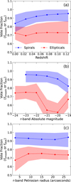 |
Fig. B.1 Variation in fsmooth for ellipticals, and fdisk for spirals, as a function of (from top to bottom) redshift, absolute magnitude in the r band and Petrosian radius (in arcseconds). |
Finally, we show in Fig. B.3 the lightGBM performance when using the "smooth" and "disk-feature" subsamples as training set. Notably, the performance is considerably worse than when we use the elliptical and spiral subsamples. While the accuracy for disk-feature is similar in Figs. 8 and B.3, the major difference is found in the counterpart. Again, this reinforces our suggestion that the separation between "smooth" and "disk-feature" is considerably subjective, and does not link directly to the elliptical-spiral separation, especially in the case of ellipticals.
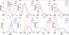 |
Fig. B.2 Nonparametric indices distribution for the smooth (dashed red), disk-feature (dashed blue), elliptical (solid red), and spiral (solid blue) subsamples. In each panel we also show the energy distance value for the comparison between smooth and elliptical distributions (in red), and between disk-feature and spiral distributions (in blue). Notably, even though adopting a considerable restrictive threshold for the smooth and diskfeature subsamples, there are significant differences in the metrics distribution. |
Appendix C Comparison of spectroscopic and photometric redshifts
In this appendix we present the comparison between spectroscopic and photometric redshift, which justifies our choice of applying a redshift threshold in our sample, even though using a photometric redshift. In Fig. C.1 we show the normalized density of galaxies in the zspec versus zphot diagram. The plot encompasses a total of 819,043 galaxies. The dashed red lines denote the interquartile range (IQR), the solid red line shows the median at each zspec, and the dotted white line shows the threshold we adopt in this work. Notably, in the local Universe (z < 0.3) both quantities show excellent agreement, ensuring that we are not introducing bias in our morphological classifications due to uncertainties in the photometric redshift.
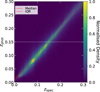 |
Fig. C.1 Number density of galaxies in the zspec vs. zphot diagram. The solid and dashed red lines denote the median and IQR of the distribution at a given zspec. The agreement between zspec vs. zphot ensures that we are not introducing bias in our morphological classification due to adopting a cut in photometric redshift. |
Appendix D Metrics definition
The galmex package computes a comprehensive set of nonparametric morphological indices, each designed to capture different aspects of galaxy structure. Below we summarize their definitions:
-
Concentration (C): Quantifies how centrally concentrated the light distribution is (Bershady et al. 2000). It is defined as
 (D.1)
(D.1)where r20 and r80 are the radii enclosing 20% and 80% of the total flux, respectively. Larger values correspond to more bulge-dominated systems.
-
Asymmetry (A): Measures the degree of 180° rotational symmetry (Conselice et al. 2000). It is computed as
 (D.2)
(D.2)where I(i, j) is the galaxy flux, I180(i, j) is the image rotated by 180° about a center (xc,yc), and the second term subtracts the contribution from background noise estimated in a representative segment (B) in the image containing only background pixels. The galaxy center is iteratively adjusted to minimize the galaxy term.
-
Shape asymmetry (AS): Similar to A, but applied to the binary segmentation map instead of the flux image (Pawlik et al. 2016). Measures rotational asymmetry in the segmentation mask rather than in the flux distribution, thereby enhancing sensitivity to faint asymmetric structures such as tidal features (Pawlik et al. 2016). The shape asymmetry is defined as
 (D.3)
(D.3)where M(i, j) is the binary segmentation map, M180(i, j) is its 180° rotation about the galaxy center, and Npix is the number of pixels in the mask. AS ranges from 0 for perfectly symmetric masks to 1 for completely asymmetric ones, and is particularly effective at identifying mergers and disturbed morphologies.
-
Smoothness (S): this measures the fraction of light in high-frequency structures (Conselice 2003). It is defined as
 (D.4)
(D.4)where IS (i, j) is a smoothed version of the image (in this case, convolved with a boxcar filter of width 0.25 RP). Therefore, high values of smoothness actually means a higher degree of clumpiness. Unlike the original definition, we omit the factor of 10 to ensure that it will be in range 0 to 1, similar to the other metrics.
-
Second-order moment of light (M20): Measures the spatial distribution of the brightest regions (Lotz et al. 2004). The total second-order moment is
![Mathematical equation: M_{\rm tot} = \sum_i f_i \left[ (x_i - x_c)^2 + (y_i - y_c)^2 \right],](/articles/aa/full_html/2026/05/aa58260-25/aa58260-25-eq12.png) (D.5)
(D.5)where fi is the flux in pixel i, and (xc, yc) is the galaxy center. M20 is then
 (D.6)
(D.6)More negative values indicate compact, bulge-like structures, while higher values trace extended or clumpy star formation.
-
Shannon entropy (E): Quantifies the uniformity in the flux distribution (Ferrari et al. 2015). Let pi = fi/Σjfj be the normalized flux distribution. Then
 (D.7)
(D.7)where Np is the number of bins used in computation. Differently from previous works, instead of fixing the number of bins for all galaxies, we define the bin width for each galaxy using the relation IQR/N1/3, where IQR is the interquartile range (Q75-Q25) and N is the number of pixels in the segmentation mask. Lower entropy values correspond to centrally concentrated systems, while higher values indicate more uniform, disk-like distributions.
-
Gini index (G): Measures the inequality of the flux distribution across pixels (Lotz et al. 2004). For pixel fluxes fi sorted in ascending order,
 (D.8)
(D.8)where f̄ is the mean pixel flux. G ranges from 0 (uniform distribution) to 1 (all flux in one pixel). Bulge-dominated systems tend to have high G.
-
Gradient pattern asymmetry (G2): Based on gradient pattern analysis, G2 measures bilateral asymmetries in the image gradient field (Rosa et al. 2018). The gradient vector field is constructed across the image, pairing vectors equidistant from the galaxy center. Symmetric pairs are discarded, while asymmetric vectors are used to define the “confluence” parameter
 (D.9)
(D.9)where
 are the asymmetric vectors. The G2 index is then given by
 (D.10)
where VA is the number of asymmetric vectors, V the total number of pixels, and cf the confluence correction.
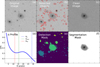 |
Fig. E.1 Illustration of the galmex preprocessing steps. Panels show the original image (a), object detection (b), the clean image (c), the Petrosian profile with key radii marked (Rp, Rkron, R50; d), the detection mask (e), and the final segmentation mask used for morphological measurements (f). |
Appendix E Description of adopted image preprocessing
Figure E.1 shows an example of the performance of the preprocessing pipeline adopted.
Appendix F The effect of aperture geometry in Petrosian radius estimates
The Petrosian radius is commonly defined as the radius rP at which the ratio between the mean surface brightness in an annulus around r and the mean surface brightness within r reaches a fixed value, ηcrit (typically ηcrit = 0.2):
![Mathematical equation: \eta(r) \equiv \frac{\langle I \rangle_{[0.8\,r,\,1.25\,r]}} {\langle I \rangle_{< r}} = \eta_{\rm crit}.](/articles/aa/full_html/2026/05/aa58260-25/aa58260-25-eq19.png) (F.1)
(F.1)
In practice, most implementations use circular apertures, i.e., r is the circular radius and the annulus is a circular ring. However, galaxies are generally not circularly symmetric. For an intrinsically flattened galaxy with semi-major axis a and semi-minor axis b = qa (q = b/a < 1), the isophotes are better described by ellipses. In that case, the “natural” Petrosian radius is an elliptical semi-major axis rP,ell measured in elliptical coordinates.
When circular apertures are used for an intrinsically elliptical system, the Petrosian annulus inevitably includes a substantial fraction of pixels that belong mostly to the sky background or to unrelated sources (“trash” pixels). A simple way to see this is to compare a circular annulus with radius r = a to an elliptical annulus with the same semi-major axis a and axis ratio q. The area of the circular annulus scales as Acirc ∝ πr2, whereas the area of the corresponding elliptical annulus scales as Aell ∝ πab = πqa2. For a given a, only a fraction ≃ q of the circular annulus overlaps the galaxy isophotes, while a fraction ≃1 - q samples mainly background. For a highly flattened system with q = 0.3, this implies that roughly 70 % of the pixels in the circular annulus are effectively “trash” pixels, whereas for a round galaxy q ≈ 1 this effect is negligible.
Because the Petrosian ratio η(r) is defined as a mean surface brightness in the annulus, the inclusion of a large and q-dependent fraction of background pixels systematically lowers ![Mathematical equation: $\langle I \rangle_{[0.8\,r,\,1.25\,r]}$](/articles/aa/full_html/2026/05/aa58260-25/aa58260-25-eq20.png) with respect to the elliptical case. The mean surface brightness within r, 〈I〉<r, is less affected because it is dominated by high S/N galaxy pixels. As a consequence, η(r) computed from circular apertures declines more rapidly with increasing r than the corresponding elliptical ηell(r), and the condition η(r) = ηcrit is reached at a smaller radius:
with respect to the elliptical case. The mean surface brightness within r, 〈I〉<r, is less affected because it is dominated by high S/N galaxy pixels. As a consequence, η(r) computed from circular apertures declines more rapidly with increasing r than the corresponding elliptical ηell(r), and the condition η(r) = ηcrit is reached at a smaller radius:
 (F.2)
(F.2)
with the bias increasing as the axis ratio q decreases. This behavior is highlighted in Fig. F.1, which shows the difference between the circular and elliptical Petrosian radius as a function of the axis ratio (b/a) of the object. This is calculated using our joint Sp and Ell samples. Notably, the use of circular apertures for objects with small axis ratio can introduce bias up to 5 arcseconds, which in the DECam resolution means ∼20 pixels, and can directly affect the creation of the segmentation mask, for instance. The bias is driven by geometry: for a flattened system, a circular annulus with radius equal to the semi-major axis inevitably includes a substantial number of pixels that lie beyond the galaxy isophotes, especially toward the galaxy’s outskirts. In contrast, an elliptical annulus with the same semi-major axis but matched axis ratio traces the isophotes and therefore better follows the true light distribution.
 |
Fig. F.1 Difference between the Petrosian radius estimated using elliptical and circular apertures, as a function of the axis ratio of the galaxy. Notably, the difference increases for decreasing axis ratio, highlighting the effect of adopting mismatching geometry when calculating the characteristic radii. |
Appendix G Effect of segmentation in metrics estimation
In this appendix we present how segmentation masks can affect the observed separation between Ell and Sp for each nonparametric index. Notably, the only index that does not rely on segmentation is C, thus it is not included in this analysis. In Fig. G.1 we show how the overlap (calculated through Eq. 3) between Sp and Ell distributions vary as a function of chosen segmentation. We considered four methods to define the segmentation mask, and parametrized the segmentation mask through the parameter k as follows:
Circular aperture (red curve) - circle with radius k × Rp;
Elliptical aperture (green curve) - elliptise with semi-major axis k × Rp;
Intensity limited (blue curve) - only pixels with intensity greater than I(k × RP) are kept in the segmentation mask;
k sigma (magenta curve) - the segmentation mask retrieved from the SExtractor detection when using a detection threshold equal to k (note that in this case, in opposition to the others, larger k means more restrict!).
In addition, we highlight using different symbols the segmentation masks used in previous works: (1) Conselice (2003, C03, empty red circle) - where the CAS parameters are defined; (2) Lotz et al. (2004, L04, empty blue circle) - inclusion of Gini index and M20; (3) Barchi et al. (2020, B20, empty magenta circle) - where they included Shannon Entropy, and G2; and (4) this work - where we adopt the CA[AS]S + MEGG sytem as input for a machine learning method to estimate spiral probabilities (empty blue square). In particular for the AS parameter (panel b), we show only the intensity limited and k sigma results, as, by definition, the other two yields a shape asymmetry equals to 0, as can be seen from Eq. D.3.
Comparison between the different panels shows that A, AS, and S are the indices more sensitive to the choice of the segmentation mask. On the other hand, panels (d), (e), and (g) shows that M20, E, and G2 are the most stable with respect to the segmentation mask choice, which highlights these indices as more robust with respect to variations in the pixel values distribution considered. Particularly for Gini index, shown in panel (f), overlap increases with k for the ellipse and intensity limited cases, which can be explained by the inclusion of pixels "close" ' ' to the background, thus setting smaller values for the "lowest income" of a pixel. In overall, our selection of intensity ensures that we are always sampling the same portion of the galaxy luminosity profile, and the choice of k = 1.0 guarantees that we are not getting any artificial increased overlap between Sp and Ell galaxies.
Appendix H Metrics comparison with Statmorph
In this appendix we show a simple comparison between the metrics C, G, and M20 estimated using galmex and statmorph for a sample of 50 randomly selected galaxies. The C index is select due to its independence of the segmentation mask, while G and M20 are selected due to statmorph measuring those indices within a segmentation mask analog to the one adopted in this work. In overall, the comparison, shown in Fig. H.1, reveals agreement between the codes, and deviations from 1-to-1 line can be explained due to small deviations in the provided segmentation mask. Notably, the major advantage of galmex over statmorph is the flexibility of the first. For each metric, in galmex, the user can select the "rule" used to define the segmentation mask, whilst this is hard coded in statmorph. Additionally, all the preprocessing steps can be easily fine tuned within the galmex graphical interface. Therefore, this test shows that the flexibility of galmex comes with no cost with respect to reliability of the metrics.
Appendix I Example table
In this appendix we present the structure of the catalog containing galaxy properties and nonparametric indices measured with galmex for the ∼1.7 million galaxies described in Sect. 2. Table I.1 shows the description of each column of the catalog made public, whereas Tables I.2 and I.3 show the description of warnings and errors, respectively.
Description of the columns of the provided catalog.
Decoding of the warn_mask bitmask.
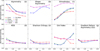 |
Fig. G.1 Variation in the overlap between Sp and Ell galaxies distributions for each segmentation-mask dependent nonparametric index (each panel). We present the results for four different types of segmentation (each colored curve), and highlight the choice of previous works in the literature in comparison to the adopted in this work (non-filled symbols). See the text for the definition of the meaning of k for each segmentation method. |
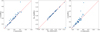 |
Fig. H.1 Comparison between the C (top panel), G (middle panel), and M20 (bottom panel) metrics estimated using the galmex (y-axis) and statmorph (x-axis) packages. Notably, both show good agreement with respect to the estimated values, irrespective of the panel considered. |
Meaning of the err_code values.
All Tables
All Figures
|
Fig. 1 Detection completeness as a function of the SEXTRACTOR detection threshold, k (in units of the background rms), for simulated Sérsic galaxies at different S/N. Solid lines show the median completeness across 1000 realizations per S/N; shaded bands indicate the 1σ scatter. The vertical dashed line marks our adopted threshold k = 1, which maintains ≳70% completeness for S/N ≥ 8 while limiting spurious detections. |
| In the text | |
|
Fig. 2 anel a: detection completeness in the 〈μ2Re〉 vs. detection threshold. Panels b-d: average difference between true and measured central position, eccentricity, and position angle, respectively, in the same grid as panel (a). We also highlight two different lines: (1) the dashed black line shows the detection threshold adopted in our pipeline; and (2) the dashed red line shows the conservative threshold in surface brightness, such that we can still recover reliable galaxy properties. |
| In the text | |
|
Fig. 3 Distribution of GZ 1 selected spiral and elliptical subsamples in the fsmooth versus fdisk (see text for the definition) diagram, according to GZ DECaLS results. The dashed black line shows the expected anticorrelation line. |
| In the text | |
|
Fig. 4 Recovery of characteristic radii across size-flux space. Each panel shows the map of the average absolute difference (in arcsec) between the measured and reference values of a given radius - R20 (a), R50 (b), R80 (c), RP (d) in the apparent magnitude vs. Re. The dashed red lines define the approximate average surface brightness when assuming a circular (q = 1) Sérsic profile. The hatched region above the 〈μ2Re〉 denotes the adopted threshold in this work. Galaxies with a surface brightness smaller than 26 mag s−2 can yield unreliable shape parameters and characteristic radii. In particular, the hatched region overlaps significantly with the region in which the error in RP exceeds 1 arcsec (∼4 pixels). This effect is more visible in RP due to it having the outermost radii in comparison to the others, and thus being more prone to background contamination. |
| In the text | |
|
Fig. 5 Distribution of spiral (blue curves) and elliptical (red curve) galaxies in 2D diagrams combing the different nonparametric indices. In each panel, we also include the overlap between the spiral and elliptical distributions, which was calculated using Eqs. (3) and (4) for histograms and 2D diagrams, respectively. |
| In the text | |
|
Fig. 6 Metrics variations with respect to CNN-based T-Type for the Sp (blue) and Ell (red) subsamples. We highlight that, although both the Sp and Ell classification, and T-Type are based on SDSS data (Galaxy Zoo 1 and 2, respectively), our results show consistency even when using DECam observations. |
| In the text | |
|
Fig. 7 Metrics variation in the smooth debiased vs. disk-feature debiased diagram. In this case we merge the spiral and elliptical subsamples in order to get a full picture of the metrics variation across this diagram. |
| In the text | |
|
Fig. 8 Results of LightGBM using the nonparametric indices as input, and trained in the GZ 1 selected spirals and ellipticals. Panels a and b: ROC curve and the precision-recall curve, respectively. Within these two panels, we also add the area under the curve (AUC) and the mean AP. Panel c: calibration curve, highlighting that our method aligns well with the expected 1 to 1 line, ensuring that our method is able to provide calibrated probabilities. Panel d: row-normalized confusion matrix. Panel e: log-loss function. See the text for a description on why there is a difference between the train and validation. Panel f: predicted spiral probability for galaxies in our test subsample. Notably, our method shows high accuracy. |
| In the text | |
|
Fig. 9 Sanity check of classifier performance as a function of observational regime. Receiver operating characteristic (ROC) curves for the spiral vs. smooth classifier evaluated in bins of (a) apparent size, using the Petrosian radius (arcsec), and (b) r band Petrosian magnitude. Curves show the mean ROC across cross-validation folds, with shaded regions indicating the ±1σ scatter between folds; the corresponding AUC values (mean ± standard deviation) are listed in the legend for each bin. Performance remains high across the full range, with the expected mild degradation toward the smallest, and faintest galaxies where morphology measurements are noisier and resolution is lower. |
| In the text | |
|
Fig. 10 SHapley Additive exPlanations (SHAP) summary plot for the LightGBM model predicting spiral galaxy classification. Each point represents the SHAP value of a single feature for one galaxy, showing its impact on the model output. The horizontal axis indicates the contribution (positive or negative) to the prediction, while the vertical axis lists the most important features ranked by overall impact. The color gradient encodes the feature value from low (blue) to high (red), highlighting how different ranges of feature values drive the prediction toward or away from the spiral class. |
| In the text | |
|
Fig. B.1 Variation in fsmooth for ellipticals, and fdisk for spirals, as a function of (from top to bottom) redshift, absolute magnitude in the r band and Petrosian radius (in arcseconds). |
| In the text | |
|
Fig. B.2 Nonparametric indices distribution for the smooth (dashed red), disk-feature (dashed blue), elliptical (solid red), and spiral (solid blue) subsamples. In each panel we also show the energy distance value for the comparison between smooth and elliptical distributions (in red), and between disk-feature and spiral distributions (in blue). Notably, even though adopting a considerable restrictive threshold for the smooth and diskfeature subsamples, there are significant differences in the metrics distribution. |
| In the text | |
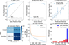 |
Fig. B.3 Similar to Fig. 8 but using the smooth and disk-feature as training samples. |
| In the text | |
|
Fig. C.1 Number density of galaxies in the zspec vs. zphot diagram. The solid and dashed red lines denote the median and IQR of the distribution at a given zspec. The agreement between zspec vs. zphot ensures that we are not introducing bias in our morphological classification due to adopting a cut in photometric redshift. |
| In the text | |
|
Fig. E.1 Illustration of the galmex preprocessing steps. Panels show the original image (a), object detection (b), the clean image (c), the Petrosian profile with key radii marked (Rp, Rkron, R50; d), the detection mask (e), and the final segmentation mask used for morphological measurements (f). |
| In the text | |
|
Fig. F.1 Difference between the Petrosian radius estimated using elliptical and circular apertures, as a function of the axis ratio of the galaxy. Notably, the difference increases for decreasing axis ratio, highlighting the effect of adopting mismatching geometry when calculating the characteristic radii. |
| In the text | |
|
Fig. G.1 Variation in the overlap between Sp and Ell galaxies distributions for each segmentation-mask dependent nonparametric index (each panel). We present the results for four different types of segmentation (each colored curve), and highlight the choice of previous works in the literature in comparison to the adopted in this work (non-filled symbols). See the text for the definition of the meaning of k for each segmentation method. |
| In the text | |
|
Fig. H.1 Comparison between the C (top panel), G (middle panel), and M20 (bottom panel) metrics estimated using the galmex (y-axis) and statmorph (x-axis) packages. Notably, both show good agreement with respect to the estimated values, irrespective of the panel considered. |
| In the text | |
Current usage metrics show cumulative count of Article Views (full-text article views including HTML views, PDF and ePub downloads, according to the available data) and Abstracts Views on Vision4Press platform.
Data correspond to usage on the plateform after 2015. The current usage metrics is available 48-96 hours after online publication and is updated daily on week days.
Initial download of the metrics may take a while.