| Issue |
A&A
Volume 709, May 2026
|
|
|---|---|---|
| Article Number | A27 | |
| Number of page(s) | 13 | |
| Section | Planets, planetary systems, and small bodies | |
| DOI | https://doi.org/10.1051/0004-6361/202558102 | |
| Published online | 29 April 2026 | |
WD 1054-226 revisited: A stable transiting debris system
1
Observatoire Astronomique de l’Université de Genève,
Chemin Pegasi 51b,
1290
Versoix,
Switzerland
2
Lund Observatory, Division of Astrophysics, Department of Physics, Lund University,
Box 118,
22100
Lund,
Sweden
3
Departamento de Astrofísica, Universidad de La Laguna (ULL),
38206
La Laguna, Tenerife,
Spain
4
Instituto de Astrofísica de Canarias (IAC),
38205
La Laguna, Tenerife,
Spain
5
McDonald Observatory,
Fort Davis,
TX
79734,
USA
6
Department of Multi-Disciplinary Sciences, Graduate School of Arts and Sciences, The University of Tokyo,
3-8-1 Komaba, Meguro,
Tokyo
153-8902,
Japan
7
Department of Physical Sciences, Ritsumeikan University, Kusatsu,
Shiga
525-8577,
Japan
8
Astrobiology Center,
2-21-1 Osawa, Mitaka,
Tokyo
181-8588,
Japan
9
National Astronomical Observatory of Japan,
2-21-1 Osawa, Mitaka,
Tokyo
181-8588,
Japan
10
Astronomical Science Program, Graduate University for Advanced Studies,
SOKENDAI, 2-21-1, Osawa, Mitaka,
Tokyo
181-8588,
Japan
11
Instituto de Astrofísica de Andalucía (IAA-CSIC), Glorieta de la Astronomía s/n, Genil,
18008
Granada,
Spain
12
INAF-Palermo Astronomical Observatory,
Piazza del Parlamento, 1,
90134
Palermo,
Italy
13
Graduate School of Social Data Science, Hitotsubashi University,
2-1 Naka, Kunitachi,
Tokyo
186-8601,
Japan
14
Komaba Institute for Science, The University of Tokyo,
3-8-1 Komaba, Meguro,
Tokyo
153-8902,
Japan
15
Okayama Observatory, Kyoto University,
3037-5 Honjo, Kamogatacho, Asakuchi,
Okayama
719-0232,
Japan
★ Corresponding author: This email address is being protected from spambots. You need JavaScript enabled to view it.
Received:
13
November
2025
Accepted:
4
March
2026
Abstract
Context. A growing number of white dwarfs (WDs) exhibit one or more signs of remnant planetary systems, including transits, infrared excesses, and atmospheric metal pollution. WD 1054-226 stands out for its unique, highly structured, and persistent photometric variability.
Aims. We investigate the long-term stability and nature of the periodic signals observed in WD 1054-226 to better understand the origin and evolution of its transiting material.
Methods. We analysed all available TESS light curves from Sectors 9, 36, 63, and 90 using Lomb–Scargle, box-least-squares, and Gaussian process periodogram analyses. We complemented them with multi-band, high-cadence ground-based photometry from LCOGT, MuSCAT2, ALFOSC, and ProEM to test for a colour dependence and confirm the periodicities.
Results. We confirm the persistence of the previously reported 25.01 h and 23.1 min periodicities over a six-year baseline. The 25.01 h signal shows some temporal evolution, while the 23.1 min dips are highly coherent on long timescales. The previously reported transient 11.4 h feature was only detected in early TESS sectors and is absent in recent data. No significant colour dependence is found in the ground-based observations.
Conclusions. The stability of the 25.01 h and 23.1 min signals indicates a long-lived, dynamically sculpted debris structure around WD 1054-226. The lack of a colour dependence implies a high optical depth, consistent with an opaque, edge-on debris ring rather than an optically thin dust population. This makes WD 1054-226 a key laboratory for testing models of remnant planetary systems around WDs.
Key words: techniques: photometric / stars: individual: WD 1054-226 / white dwarfs
© The Authors 2026
 Open Access article, published by EDP Sciences, under the terms of the Creative Commons Attribution License (https://creativecommons.org/licenses/by/4.0), which permits unrestricted use, distribution, and reproduction in any medium, provided the original work is properly cited.
This article is published in open access under the Subscribe to Open model. This email address is being protected from spambots. You need JavaScript enabled to view it. to support open access publication.
1 Introduction
When a star similar to the Sun ends its life, it sheds its outer layers and contracts into a white dwarf (WD). While the inner planetary system is engulfed, outer planets and minor bodies can survive and later perturb one another. This causes material to be scattered onto the WD (e.g. Debes & Sigurdsson 2002; Bonsor et al. 2011; Mustill & Villaver 2012; Veras et al. 2014; Mustill et al. 2018; Smallwood et al. 2021; Veras et al. 2024). Those planets and minor bodies that pass within the Roche limit are tidally disrupted, generating compact dusty and gaseous discs (Jura 2003; Gänsicke et al. 2006). Heavy element pollution in WD atmospheres (Zuckerman et al. 2003; Koester et al. 2014; Ould Rouis et al. 2024), along with infrared excesses consistent with circumstellar dust discs (Zuckerman & Becklin 1987; Graham et al. 1990; Reach et al. 2005; Jura et al. 2007; Wilson et al. 2019; Madurga Favieres et al. 2024; Murillo-Ojeda et al. 2026), and circumstellar gas emission (Gänsicke et al. 2006; Manser et al. 2020; Saker et al. 2025), provide strong evidence for ongoing accretion of such material. Recent James Webb Space Telescope (JWST) observation using the Mid-Infrared Instrument (MIRI) has revealed a wide variety of dust mineralogies, including tentative silica glass signatures, which indicate high-temperature processing and collisional replenishment of small grains (Farihi et al. 2025).
In rare cases, fragments can be observed to directly transit their WD host. The first and best-studied example, WD 1145+017, showed multiple dust clouds orbiting near the Roche limit with a period of ≈4.5 h (Vanderburg et al. 2015; Aungwerojwit et al. 2024). Since then, over a dozen similar systems have been reported (e.g. Vanderbosch et al. 2020; Guidry et al. 2021; Vanderbosch et al. 2021; Aungwerojwit et al. 2024; Hermes et al. 2025; Bhattacharjee et al. 2025; Guidry et al. 2025), demonstrating diverse activity levels and dynamical pathways. However, only six of these systems have measured orbital periods. Theoretical models suggest that these phenomena (discs, transits and pollution) arise from gravitational perturbations by surviving planets (Bonsor et al. 2011; Mustill et al. 2018), leading to either full tidal disruption of an asteroid or comet within the Roche limit or to alternative outcomes. For example, secular and scattering perturbations can trigger repeated partial disruptions of planets or asteroids (Li et al. 2021; Kurban et al. 2024), while Li et al. (2025b) showed that bodies scattered to orbital pericentres just outside the Roche limit may undergo tidal circularisation to short-period (≈ 10 h–1 d) orbits. The authors showed that this mechanism can account for the orbital periods observed in systems such as WD 1145+017. A companion study suggested that tidal heating during this evolution might induce volcanism, producing dust-rich ejecta and distinctive occultations (Li et al. 2025a).
The nearby metal-polluted WD 1054-226 displays uniquely structured and persistent photometric variability (Farihi et al. 2022; Robert et al. 2024). As described in Farihi et al. (2022), WD 1054-226 shows quasi-continuous dimming events that repeat with remarkable precision in a 25.01 h period, but with evolving morphology and variability at multiple harmonics, in particular, the 65th harmonic at 23.1 min. This variability, drifting transit features that suggest additional periodicities, and the absence of un-occulted starlight have been interpreted by Farihi et al. (2022) as produced by an opaque, edge-on debris structure occulting the WD, which is subject to perturbations from a nearby massive body, such as a large asteroid fragment. Recent studies also suggested that the 25.01 h signal might be consistent with a partially circularised planetesimal orbit (Li et al. 2025b) or with volcanically active bodies shedding dust in a narrow ring (Li et al. 2025a).
The stability and regularity of WD 1054-226 distinguish it from other transiting debris systems, making it a rare laboratory for testing models of evolved planetary systems. The published observational baseline for this system extends only over four years. Systems like this have been observed only recently, and little is known so far about their long-term evolution or stability, although the small number of known systems show a range of temporal behaviours. The transits of the archetypal system WD 1145+017 have disappeared, or at least reduced in depth to become undetectable, after several years (Aungwerojwit et al. 2024). Like WD 1054-226, ZTF J0328-1219 shows complex transit features without an obvious out-of-transit baseline, but its periodicities (around 9.9 and 11.2 hours) change both within and between Transiting Exoplanet Survey Satellite (TESS) sectors (Vanderbosch et al. 2021). SBSS 1232+562 has undergone several month-long dimming events, after the last of which, a 14.8-hour periodicity briefly appeared (Hermes et al. 2025). ZTF J1944+4557 shows cleaner transits with a clear flat baseline between the transit events, although they are still more complex than the single transit per cycle (here 4.97 hours) seen for transits of planets; these transits were observed in 2023 and 2025, but temporarily disappeared in 2024 (Guidry et al. 2025). Long-term monitoring of more systems is therefore essential to constrain the typical timescales on which these systems change, if indeed they all do. We present new observations and an analysis of WD 1054226 to constrain the nature of the transiting material and its role in the late stages of planetary system evolution.
2 Observations
2.1 TESS photometry
The WD 1054-226 (TIC 415714190) was observed by TESS (Ricker et al. 2015) in Sector 9 at a cadence of 2 min and in Sectors 36, 63, and 90 at a cadence of 20 sec. We used the publicly available Pre-search Data Conditioning (PDC) light curves (Smith et al. 2012; Stumpe et al. 2012, 2014) produced by the Science Processing Operations Center (SPOC: Jenkins et al. 2016) at NASA Ames Research Center, downloaded from the Mikulski Archive for Space Telescopes1.
2.2 Ground-based photometry
2.2.1 LCOGT/Sinistro
We observed WD 1054-226 in the SDSS i′ band (617 to 894 nm) using the Sinistro cameras installed at the 1 m telescopes from the Las Cumbres Observatory Global Telescope (LCOGT; Brown et al. 2013) between 14 December 2022 and 27 June 2025, covering observing windows from 2.13 to 7.48 hours. Details of the observations are reported in Table A.1. The SDSS i′-band images were calibrated by the standard LCOGT BANZAI pipeline (McCully et al. 2018), and the photometry was reduced with our pipeline following standard photometry practices (Parviainen et al. 2019). The reduced i′-band photometry from LCOGT and all the other instruments is shown in Fig. 1.
2.2.2 TCS/MuSCAT2
We observed WD 1054-226 in the g′ (400–550 nm), r′ (550–700 nm), i (700–820 nm), and zs (820–920 nm) bands using the multi-band imager MuSCAT2 (Narita et al. 2019) mounted on the 1.5 m Telescopio Carlos Sánchez (TCS) at Teide Observatory, Spain, between 24 January 2023 and 12 March 2024, with observing windows lasting from 2.0 to 3.7 hours. All the MuSCAT2 data were reduced by the MuSCAT2 pipeline (Parviainen et al. 2019). The pipeline performs standard calibrations (dark and flat-field corrections) and aperture photometry. Three nights (25 January 2023, 5 March 2023, and 31 March 2023) were cloudy, and the photometry for these nights was not included in the analysis. The multi-colour photometry from MuSCAT2 and all the other instruments is shown in Fig. 2, and the white-light curve from MuSCAT2 with the colour differences is shown in Fig. B.1.
2.2.3 Struve/ProEM
We observed WD 1054-226 semi-simultaneously in SDSS g′ and i′ using the ProEM frame-transfer photometer mounted on the 2.1 m Otto Struve Telescope at McDonald Observatory, Texas, USA, on 5 January 2024 and 6 January 2024. The photometry was reduced with our pipeline in the same way as the LCOGT photometry.
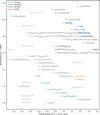 |
Fig. 1 All i-band light curves ordered into groups and phase-folded to the 25.01 h period. The reference time for the phase folding is 2459928.85. The y-offset of the light curves in each group correspond to the 25.01 h period signal cycle. |
2.2.4 NOT/ALFOSC
We observed WD 1054-226 semi-simultaneously in the SDSS i′ and g′ bands using the Alhambra Faint Object Spectrograph and Camera (ALFOSC) instrument installed at the 2.56 m Nordic Optical Telescope (NOT) at the Roque de los Muchachos Observatory on La Palma, Spain, on 18 March 2023. The photometry was reduced with our pipeline in the same way as the LCOGT photometry.
3 Methods
3.1 Lomb–Scargle and box-least-squares periodograms
Previous searches for periodic signals in the photometry of WD 1054-226 used Lomb–Scargle (LS; Lomb 1976; Scargle 1982) and box-least-squares (BLS; Kovacs et al. 2002) periodograms (Farihi et al. 2022; Robert et al. 2024). We repeated these analyses using our ground-based photometry and the new TESS observations.
For the LS search, we used the astropy implementation to identify sinusoidal periodicities in the TESS and ground-based data sets using the standard normalisation in the range 10 min to 50 days and 10 min to 3 days, respectively. The false-alarm probability level was calculated using the astropy implementation with the method described in Baluev (2008). To search for periodic transit-like features in the TESS photometry, we employed the BLS algorithm implemented in the Open Exoplanet Transit Search pipeline (OpenTS; Pope et al. 2016) using the PyTransit transit model (Parviainen 2015, 2020; Parviainen & Korth 2020). The BLS search was divided into short- and long-period searches, and we explored trial periods of 0.007–0.2 days and 0.2–2 days, respectively.
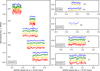 |
Fig. 2 Multi-colour photometry from MuSCAT2, ProEM, and ALFOSC shown for filters g′ (blue), r (green), i, and i′ (yellow), and zs (red) and phase-folded to the 25.01 h period. The reference time for the phase folding is 0.0. The MusCAT2 photometry is binned to 3 min, the ProEM photometry to 2 min, and the ALFOSC photometry is not binned. The y-offset of the light curves corresponds to the 25.01 h period signal cycle. |
3.2 Gaussian process period analyses
3.2.1 Gaussian process kernel
The LS periodogram is optimised for detecting sinusoidal variability. On the other hand, the BLS periodogram is better suited for identifying periodic transit-like signals, where the duration of the dip is short compared to the period.
We adopted an additional approach and modelled the photometry using a Gaussian process (GP; Rasmussen & Williams 2006) consisting of an aperiodic component and up to three quasi-periodic components. The full covariance kernel is
![Mathematical equation: $\[\begin{aligned}k(\tau)= & \underbrace{\sigma_{a p}^2\left(1+\frac{\sqrt{3} \tau}{\rho}\right) \exp \left(-\frac{\sqrt{3} \tau}{\rho}\right)}_{\text {Aperiodic}} \\& +\sum_{i=1}^N \underbrace{\sigma_i^2 \exp \left(-\frac{\tau^2}{2 \ell_i^2}-\Gamma_i ~\sin ^2\left(\frac{\pi \tau}{P_i}\right)\right)}_{\text {Quasi-periodic}},\end{aligned}\]$](/articles/aa/full_html/2026/05/aa58102-25/aa58102-25-eq1.png) (1)
(1)
where τ = |t − t′| is the time lag between data points, N ∈ {1, 2, 3} is the number of periodic signals, and σ is the amplitude of the component. The aperiodic variability was modelled with a Matérn-3/2 covariance function, governed by the characteristic timescale ρ. The quasi-periodic signals were modelled by multiplying an exponential-sine-squared kernel with a squared-exponential kernel. This introduced an evolutionary timescale, ℓ, that dictates the stability of the periodicity; a large ℓ (ℓ ≫ P) enforces a strictly periodic persistent signal, while a smaller ℓ allows the signal phase or amplitude to evolve or decay over time. The shape of the periodic feature was controlled by the characteristic inverse-length scale, Γ. Low values of Γ constrain the periodic component to smooth sinusoidal variations, while high values of Γ allow for sharp pulse-like features with rich harmonic content. This formulation allowed us to model a wide range of behaviours, including long-timescale stochastic variability, sharp transit-like dips, and quasi-periodic signals with an evolving morphology.
3.2.2 Period search with Gaussian processes
We began by carrying out period searches using the TESS data and the ground-based LCOGT data from January and March 2024. The searches were formulated as hypothesis tests between three competing models: H0, in which the variability is explained entirely by an aperiodic process; H1, in which the variability is explained by an aperiodic process and a single quasi-periodic signal with period p1; and H2, in which the variability is explained by an aperiodic process and two quasi-periodic signals with periods p1 and p2.
We evaluated these hypotheses using Bayesian information criterion (BIC) periodograms. First, we fitted the H0 model by optimising the Matérn-3/2 hyperparameters and computing the maximum log-likelihood. We then performed a period search by evaluating H1 over a grid of trial periods p1. At each trial period, we fixed the aperiodic hyperparameters to their best-fit H0 values and optimised the quasi-periodic kernel hyperparameters over a predefined grid. The resulting ΔBIC = BICH1 − BICH0 identifies periods where the inclusion of a periodic component significantly improves the fit. A lower ΔBIC indicates stronger evidence in favour of H1, where ΔBIC < −6 can be considered strong evidence, and ΔBIC <-10 very strong (Kass & Raftery 1995, adopting 2 ln B10 ≈ −ΔBIC). For H2, we carried out a conditional search for secondary periodicities: we included a known primary period p1 in the model and scanned for an additional period p2, which allowed us to distinguish genuine secondary signals from harmonics of the dominant periodicity.
We modelled the GPs using the George package (Ambikasaran et al. 2016) with the basic solver rather than the Hierarchical Off-Diagonal Low-Rank (HODLR) approximation, so the computational cost is dominated by the 𝒪(N3) scaling of the covariance matrix inversion. To mitigate this, we adopted different strategies for the short- and long-period searches. For short periods (5–60 min), we did not bin the data in time, but instead divided the light curves into chunks of n data points at most and computed the total log-likelihood as the sum over the individual chunks. For long periods (3–29 h), we binned the TESS light curves into 22-minute intervals, keeping the total number of points per sector at about 1500; the ground-based light curves were binned into 4-minute intervals.
The periodograms were calculated separately for each TESS sector and separately for the LCOGT observations from January and March 2024. The searches were limited to two periodicities at most at each timescale, as our tests found no evidence for additional periodic signals.
3.2.3 Model refinement and comparison
The BIC periodograms identify candidate periods, but rely on grid searches with fixed aperiodic hyperparameters and approximate optimisation. To refine the results, we performed full GP optimisations for the most significant periods. For each candidate period or period pair, we optimised all hyperparameters jointly and recomputed the BICs for H0, H1, and H2. The optimisation uses the differential evolution (DE; Storn & Price 1997; Price et al. 2005) algorithm implemented in PyTransit (Parviainen 2015). The resulting models were then compared to determine which set of periodicities best explains the data.
3.2.4 Posterior sampling
For the best-fitting models, we estimated the full posterior distributions of the GP hyperparameters using a Markov chain Monte Carlo sampling. We used the affine-invariant sampler implemented in emcee (Foreman-Mackey et al. 2013), initialising the walkers at the global posterior mode found by the DE optimisation. The sampling was carried out with 50 walkers for 5000 steps. We discarded the first 4000 steps as burn-in and retained the final 1000 steps as the posterior sample.
3.3 Colour dependence
Our ground-based photometry includes observations obtained in multiple passbands, either simultaneously or semi-simultaneously (see Sect. 2.2). We investigated whether the depths of the light-curve dips depended on colour, which might provide insights into the composition and size distribution of the material that causes the dips (e.g. Alonso et al. 2016; Xu et al. 2018).
The analysis parallels the approach of Farihi et al. (2022). First, we resampled all passbands onto a common time grid to enable a direct comparison; this step is required even for the MuSCAT2 data due to differences in exposure times. We then examined the correlations between fluxes across the passbands and assessed whether they showed significant non-linearity or deviations from unity, which would indicate a colour-dependent dip depth.
4 Results
4.1 TESS period search
We analysed all available TESS photometry using the BLS, LS, and GP approaches.
The BLS transit search was performed per sector and across multiple sectors using the 20 s and 2 min cadence data. The long-period BLS search identified an 8.34 h signal in Sector 9, consistent with a harmonic of the 25.01 h modulation, as well as the 25.01 h periodicity itself in Sectors 36, 63, and 90, both individually and in the combined multi-sector searches. The short-period BLS search identifies the 23.1 min signal in all individual sectors and in a search combining all the TESS sectors.
The LS search was performed using the 2 min cadence alone; the periodograms (Fig. 3) recover the two dominant periodicities previously reported by Farihi et al. (2022): the 23.1 min signal and the 25.01 h fundamental period. In addition, a secondary signal with a period of either 5.7 h or 11.4 h was detected in Sectors 9 and 36, in agreement with the findings from Farihi et al. (2022).
The GP period searches were carried out separately for each TESS sector using the 2 min cadence photometry. We computed the GP periodograms for long periods (3–29 h, using light curves binned into 22-minute intervals) and short periods (6–36 min, using unbinned photometry split into segments of 750 data points).
The long-period TESS results are shown in Fig. 4. The GP periodograms recover the 25.01 h signal seen in the LS analysis and a candidate periodicity at either 11.4 or 22.8 h in Sectors 9 and 36. The short-period search detects the known 23.1 min signal, but finds no other significant features. To search for secondary periodicities, we computed conditional two-period GP periodograms (right column of Fig. 4), comparing a one-period model with p1 = 25 h against a two-period model with p1 = 25 h and p2 scanned across a grid of trial periods. In Sectors 9 and 36, the best-fitting models combine the 25.01 h signal with either the 11.4 h or 22.8 h periodicity: a weak secondary signal appears in Sector 9 and becomes stronger in Sector 36. By contrast, Sectors 63 and 90 are consistent with a single-period model dominated by the 25.01 h signal, and no significant secondary periodicities are detected.
The LS and GP analyses both confirm that the known 25.01 h periodicity is the dominant stable signal throughout the TESS observations, with little risk of it being an alias of another period. However, the two methods produce slightly different results for the secondary signal in Sectors 9 and 36. The LS analysis identifies the strongest secondary peaks at 5.7 h and 11.4 h, whereas the GP analysis prefers periods of 11.4 h and 22.8 h.
To identify which long-period signals are genuinely present in each sector, we compared the BICs of competing GP models (Sect. 3.2.4): an aperiodic model, single-period models at 5.7, 11.4, 22.8, and 25.0 h, and two-period models combining the 25 h signal with each candidate secondary period. The resulting ΔBIC values are summarised in Table 1. The preferred model for Sectors 9 and 36 combines the 25.01 h and 11.4 h periodicities, while Sectors 63 and 90 are best explained by a single 25.01 h signal.
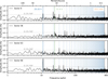 |
Fig. 3 LS periodograms of the TESS photometry from Sectors 9, 36, 63, and 90. The known 23.1 min and 25.01 h periodicities are marked with solid orange and blue lines, respectively, while the 11.4 h signal is marked with a solid green line. The dashed and dotted lines indicate harmonics of these signals using the same colour-coding. |
4.2 Ground-based period search
When we combined all available ground-based datasets, the LS analysis detected only the 23.1 min modulation, while the longer-period signals remained undetected. This is likely due to the limited temporal coverage and the strongly non-sinusoidal nature of the variability, which makes the LS method less sensitive to the 25.01 h signal. In contrast, the GP periodogram combining the January 2024 and March 2024 observations recovers both the 23.1 min and 25.01 h modulations.
We also performed separate analyses for two data subsets obtained in January 2024 and March 2024. In January, the LS periodogram again identifies the 23.1 min modulation, with additional candidate long-period signals that are most likely spurious. The GP analysis confirms the presence of the 23.1 min variability and recovers the 25.01 h signal. A weaker feature near 6.25 h is also present, but this is consistent with being an alias of the 25.01 h modulation rather than an independent period. The March 2024 data show a similar picture: the 23.1 min signal is robustly detected in the LS and GP analyses. The GP analysis detects the 25.01 h modulation, but with a lower statistical significance than in the January 2024 data, and a tentative ≈5 h signal is also present, but lacks statistical significance. Overall, the ground-based LS analysis consistently detects the 23.1 min modulation, but fails to recover the 25.01 h periodicity, which is expected given its sensitivity to sinusoidal variability.
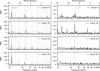 |
Fig. 4 GP periodograms for the long-period searches (3–29 h) from the TESS Sector 9, 36, 63, and 90 photometry. Left column: 1D periodograms for a single-period GP model. The plotted signal amplitude ΔBIC is defined as the difference between the BIC of the single-period GP model and that of the aperiodic GP model, i.e. ΔBIC = BIC1(p1) − BIC0. Right column: conditional 1D periodograms for a two-period GP model where p1 is fixed to 25.01 h. Here, ΔBIC = BIC2(p1 = 25.01 h, p2) − BIC1(p1 = 25.01 h). The known 25.01 h period and its harmonics are marked with solid and dashed blue lines, respectively, while the 11.4 h period and its harmonics are marked with the solid and dotted green lines. The horizontal slashed line shows the ΔBIC level of −10, which corresponds to very strong evidence in favour of the periodic signal (Kass & Raftery 1995). |
Difference in BIC (ΔBIC) relative to the best-fitting model for each TESS sector.
4.3 Gaussian process posterior analysis
We present the GP period posteriors for the best models in Table 2, the remaining hyperparameter posteriors in Fig. 5, and the median posterior GP models for the ground-based observations in Fig. 6. The period estimates for the 25.01 h and 23.1 min signals are consistent across all TESS sectors and the ground-based data. The two TESS sectors that exhibit the 11.4 h signal also agree within the uncertainties, but the signal is relatively weak in Sector 9. We found no statistically significant drifter-like features in the ground-based data after removing the GP model, including the 25.01 h and 23.1 min signals.
The hyperparameter posteriors (Fig. 5) reveal markedly different characteristics for each periodicity in the ground-based data. The 25.01 h signal has a well-constrained coherence timescale of ℓ ≈ 10 days (the 68% central credible interval for log10 ℓ is 0.85–1.5, which corresponds to an ℓ interval of 7–31 d) and a very high harmonic complexity (log10 Γ ≈ 4), consistent with a sharp, complex periodic waveform that remains coherent within each observing campaign, but evolves over the combined January–March baseline. The 23.1 min signal has a low harmonic complexity (log10 Γ ≈ −1), indicating a smooth, nearly sinusoidal waveform, and a coherence timescale with a lower bound of ℓ > 170 d (99% credible lower limit), meaning that it remains coherent over at least the full ground-based observing baseline. Its amplitude is comparable to that of the 25.01 h signal at approximately 1% of the normalised flux.
In the TESS data, the 25.01 h signal shows poorly constrained ℓ posteriors with ℓ ≳ 1, indicating coherence over timescales likely longer than the sector baseline, with log10 Γ ≈ 2. The 11.4 h signal, detected only in Sectors 9 and 36, has a short coherence timescale (ℓ ≲ 1 day) and high harmonic complexity, as expected for transit-like dips with rapidly evolving morphology. The 23.1 min signal is poorly constrained by the TESS photometry, with broad posteriors for all hyperparameters, consistent with the low signal-to-noise ratio at this cadence for a faint target. Overall, the ground-based observations provide significantly tighter constraints on the hyperparameters of the 25.01 h and 23.1 min signals than TESS, owing to their substantially higher photometric precision.
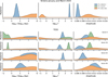 |
Fig. 5 Posterior densities for the GP model hyperparameters estimated from the ground-based LCOGT observations and from separate TESS sectors. First column: GP coherence scale. Second column: GP harmonic complexity. Third column: amplitude of the periodicity. The 11.4 h period is estimated only from the TESS Sectors 9 and 36. The ground-based posterior estimates for the 25.01 h and 23.1 min periodicities are significantly better than the TESS ones due to the significantly higher photometric precision. |
Period posterior estimates from the GP analyses.
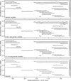 |
Fig. 6 Ground-based LCOGT observations for January and March 2024 (points with error bars) together with the GP model consisting of an aperiodic component, a 25.01 h quasi-periodic component, and a 23.1 min quasi-periodic component (black line) folded over the 25.01 h period. Top three panels: each separate GP component without the other components from the observations and the model. Bottom panel: observation residuals with respect to the full GP model. The cycle number is marked on the right, starting from the first light curve in the dataset. |
4.4 Colour dependence
Finally, we investigated the wavelength dependence of the dips using the multi-colour photometry (Fig. 2). We found no evidence of a colour dependence in the dip depths within the observational uncertainties, consistent with previous studies of WD 1054-226 (Figs. B.1 and B.2).
5 Discussion
As pointed out by Farihi et al. (2022), who analysed the TESS Sectors 9 and 36, large scatter prevents a direct detection of transiting events, but is beneficial for a frequency analysis. However, Robert et al. (2024) used a combined BLS and LS analysis and detected the 25.01 h period using Sectors 9, 36, and 63. We confirm this and the 23.1 min period, and we also report that these signals persist in Sector 90.
The 25.01 h and 23.1 min signals are now largely persistent for over 6 years (2300 days, or >2200 cycles of the 25.01 h signal), indicating that they are reasonably long-lived and not rapidly decaying transients. This is consistent with a dynamical origin in which a disc is sculpted by a nearby massive perturber, such as an asteroid, whether via waves as in Saturn’s rings or via resonant clumps. In this scenario, the 25.01 h period is that of the perturbing body, while the 23.1 min signal (at a 65:1 commensurability) is caused by resonant clumping of material, or waves launched by a 66:65 mean motion resonance at the disc edge, although both of these scenarios have qualitative challenges in explaining the shape of the light curves (see discussion in Farihi et al. 2022). Interestingly, the ratio of the 25.01 h and 23.1 min signals is very close to 65 in all TESS sectors except for Sector 36: here, the closest commensurability is 64:1, but the observed ratio lies further from the commensurability (Fig. 7); we note that the drifters were more noticeable in this sector than in the others, and this might affect the periodogram results. In these scenarios, the 25.01 h signal is expected to remain phase-coherent, as it is tied to the period and phase of the perturbing body. However, we determined a relatively low coherence time for this signal, which might arise from an evolution of its morphology rather than its phase. If the disc is sufficiently massive and flat, relatively rapid migration of the perturbing body might take place on timescales much shorter than the expected disc lifetimes of ~1 Myr (Veras et al. 2023). As an alternative scenario, the 25.01 h period might correspond to magnetically trapped dust that co-rotates with the stellar magnetosphere, as suggested for WD 1145+017 (Farihi et al. 2017) and for young main-sequence stars (Bouma et al. 2024). The stellar rotation period of >3 hours (Farihi et al. 2022) is consistent with this scenario.
The exact nature of the 23.1 min signal remains undetermined. In these dynamical scenarios, the 23.1 min signal is still expected to show phase coherence, since the zero phase should be set by the longitude of conjunction with the perturbing body. The amplitude, however, might vary, for example, as the bodies composing the disc orbit at a different frequency from the perturbing body. The coherent 23-minute signal is consistent with a constant forcing frequency, for example, from mean motion resonances with an asteroid. A possible challenge to these dynamical models comes from the relatively wide orbit of the perturbing body. Its orbital period of 25.01 h is too long to have permitted tidal circularisation, and it may possess a considerable residual eccentricity in the range 0.2–0.4 (Li et al. 2025b). This would likely render these dynamical models untenable, as such nearby mean motion resonances as the 66:65 will likely be destabilised by such a high eccentricity. However, other means exist of lowering a scattered body’s eccentricity, such as interactions with any pre-existing disc: it is not necessary that the disc material actually originates from the perturbing body (Mustill et al. 2018).
The lack of a colour dependence of the transits is in line with observations of WD 1145+017 (Alonso et al. 2016; Izquierdo et al. 2018; Xu et al. 2018), WD J0328-1219 (Gary & Kaye 2024), ZTF J1944+4557 (Guidry et al. 2025), and SBSS 1232+563 (Hermes et al. 2025), and it implies a lack of small grains in the structures transiting these stars, if the structures are in an optically thin regime (Xu et al. 2018). However, small grains should be present as they are expected to be rapidly replenished by collisions in these discs. Xu et al. (2018) argued for WD 1145+017 that small grains probably sublimate rapidly, and hence do not contribute to the opacity. On the other hand, Izquierdo et al. (2018) pointed out that small grains might be present if the optical depth is high across the whole of the transiting structures, transitioning with a rapid gradient to zero towards their edge, so there would be no noticeable optically thin regime. As with these other WDs, we found no colour dependence in the transits of WD 1054-226. For WD 1054-226, the longer orbital period and lower stellar Teff mean that the grain temperature is much lower than for WD 1145+017: we calculate a blackbody grain temperature of 320 K at P = 25 h, while accounting for inefficient cooling of sub-micron grains (Xu et al. 2018, Eq. (8)) gives an estimated grain temperature of 600 K. This is far too low for the grains to sublimate on relevant timescales: following (Xu et al. 2018), we found a sublimation lifetime of 1018 yr for 10 nm grains. This means that for WD 1054-226, sublimation cannot be invoked as a means to remove small grains. Instead, they must be present, but rendered invisible in the colour information, presumably by a high optical depth. We note that the non-detection of circumstellar gas absorption in WD 1054-226 by Farihi et al. (2022), in contrast to detections in WD 1145+017 (Xu et al. 2016; Redfield et al. 2017), would be consistent with a lack of sublimation in the former’s disc.
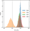 |
Fig. 7 Posterior distribution of the ratio of the 25.01 h period and the 23.1 min period estimated from the 2 min cadence TESS photometry from the four TESS sectors. All sectors lie close to the 65:1 commensurability, except for Sector 36. |
6 Conclusions
We have presented updated time-series photometry for the variable white dwarf WD 1054-226, including a new sector of TESS observations as well as multi-band ground-based photometry.
WD 1054-226 still displays significant variability with periods of 25.01 h and 23.1 min, which now have remained stable over 6 years, indicating a relatively long-lived origin. These periods appear both in an LS periodogram analysis, and when incorporating a GP to account for aperiodic variability. The 23.1 min signal remains at the 65:1 period commensurability with the 25.01 h signal, which is qualitatively consistent with the original interpretation of Farihi et al. (2022), which posits that they arise from the sculpting of a circumstellar disc by a nearby or embedded asteroid. However, in TESS Sector 36, the period ratio drifted from 65:1, which might indicate additional processes in the system or cast doubt on this interpretation.
The ground-based observations included simultaneous multi-band observations, which showed no colour dependence of the transits, as was also the case for WD 1145+017 and several similar WDs. However, for WD 1054-226, the transiting material is cool enough that rapid sublimation of small dust grains cannot be invoked. Instead, the disc of material might be optically thick at all passbands observed so far.
While a quantitative model for this system remains lacking, any such model must account for the disc’s high optical depth and the stability of the dominant frequencies.
Acknowledgements
This paper includes data collected with the TESS mission, obtained from the MAST data archive at the Space Telescope Science Institute (STScI). Funding for the TESS mission is provided by the NASA Explorer Program. STScI is operated by the Association of Universities for Research in Astronomy, Inc., under NASA contract NAS 5-26555. This work makes use of observations from the Las Cumbres Observatory global telescope network. This paper is based on observations made with the MuSCAT2 instrument, developed by ABC, at Telescopio Carlos Sánchez operated on the island of Tenerife by the IAC in the Spanish Observatorio del Teide. This paper includes data taken at the McDonald Observatory of the University of Texas at Austin. The data presented here were obtained in part with ALFOSC, which is provided by the Instituto de Astrofisica de Andalucia (IAA) under a joint agreement with the University of Copenhagen and NOT. The authors acknowledge support from the Swiss NCCR PlanetS and the Swiss National Science Foundation. This work has been carried out within the framework of the NCCR PlanetS supported by the Swiss National Science Foundation under grants 51 NF 40182901 and 51NF40205606. JK acknowledges support of the Swiss National Science Foundation under grant number TMSGI2_211697. AJM and JK acknowledge support from the Swedish Research Council (Starting Grant 2017-04945 and Project Grant 2022-04043). HP acknowledges support by the Spanish Ministry of Science and Innovation with the Ramon y Cajal fellowship number RYC2021-031798-I. VB acknowledges support from grant PID2022-137241NB-C41 funded by Agencia Estatal de Investigación of the Ministerio de Ciencia, Innovación y Universidades (MICIU/AEI/10.13039/501100011033) and ERDF/EU. E. E-B. acknowledges financial support from the European Union and the State Agency of Investigation of the Spanish Ministry of Science and Innovation (MICINN) under the grant PRE2020-093107 of the Pre-Doc Program for the Training of Doctors (FPI-SO) through FSE funds. G.M. acknowledges financial support from the Severo Ochoa grant CEX2021-001131-S and from the Ramón y Cajal grant RYC2022-037854-I funded by MCIN/AEI/1144 10.13039/501100011033 and FSE+. Funding from the University of La Laguna and the Spanish Ministry of Universities is acknowledged. This work is partly financed by the Spanish Ministry of Economics and Competitiveness through grants PGC2018-098153-B-C31. We acknowledge financial support from the Agencia Estatal de Investigación of the Ministerio de Ciencia e Innovación MCIN/AEI/10.13039/501100011033 and the ERDF “A way of making Europe” through project PID2021-125627OB-C32. This work is partly supported by JSPS KAKENHI Grant Numbers JP21K13955, JP24H00017, JP24H00248, JP24K00689, JP24K17082, and JP24K17083, JSPS Bilateral Program Number JPJSBP120249910, JST SPRING Grant Number JPMJSP2108, and JSPS Grant-in-Aid for JSPS Fellows Grant Numbers JP24KJ0241, JP25KJ0091, and JP25KJ1040.
References
- Alonso, R., Rappaport, S., Deeg, H. J., & Palle, E. 2016, A&A, 589, L6 [NASA ADS] [CrossRef] [EDP Sciences] [Google Scholar]
- Ambikasaran, S., Foreman-Mackey, D., Greengard, L., Hogg, D. W., & O’Neil, M. 2016, IEEE Trans. Pattern Anal. Mach. Intell., 38, 252 [Google Scholar]
- Aungwerojwit, A., Gänsicke, B. T., Dhillon, V. S., et al. 2024, MNRAS, 530, 117 [NASA ADS] [CrossRef] [Google Scholar]
- Baluev, R. V. 2008, MNRAS, 385, 1279 [Google Scholar]
- Bhattacharjee, S., Vanderbosch, Z. P., Hollands, M. A., et al. 2025, PASP, 137, 074202 [Google Scholar]
- Bonsor, A., Mustill, A. J., & Wyatt, M. C. 2011, MNRAS, 414, 930 [CrossRef] [Google Scholar]
- Bouma, L. G., Jayaraman, R., Rappaport, S., et al. 2024, AJ, 167, 38 [NASA ADS] [CrossRef] [Google Scholar]
- Brown, T. M., Baliber, N., Bianco, F. B., et al. 2013, PASP, 125, 1031 [Google Scholar]
- Debes, J. H., & Sigurdsson, S. 2002, ApJ, 572, 556 [NASA ADS] [CrossRef] [Google Scholar]
- Farihi, J., von Hippel, T., & Pringle, J. E. 2017, MNRAS, 471, L145 [NASA ADS] [CrossRef] [Google Scholar]
- Farihi, J., Hermes, J. J., Marsh, T. R., et al. 2022, MNRAS, 511, 1647 [NASA ADS] [CrossRef] [Google Scholar]
- Farihi, J., Su, K. Y. L., Melis, C., et al. 2025, ApJ, 981, L5 [Google Scholar]
- Foreman-Mackey, D., Hogg, D. W., Lang, D., & Goodman, J. 2013, PASP, 125, 306 [Google Scholar]
- Gänsicke, B. T., Marsh, T. R., Southworth, J., & Rebassa-Mansergas, A. 2006, Science, 314, 1908 [Google Scholar]
- Gary, B. L., & Kaye, T. G. 2024, RNAAS, 8, 173 [Google Scholar]
- Graham, J. R., Matthews, K., Neugebauer, G., & Soifer, B. T. 1990, ApJ, 357, 216 [NASA ADS] [CrossRef] [Google Scholar]
- Guidry, J. A., Vanderbosch, Z. P., Hermes, J. J., et al. 2021, ApJ, 912, 125 [NASA ADS] [CrossRef] [Google Scholar]
- Guidry, J. A., Vanderbosch, Z. P., Hermes, J. J., et al. 2025, ApJ, 992, 167 [Google Scholar]
- Hermes, J. J., Guidry, J. A., Vanderbosch, Z. P., et al. 2025, ApJ, 980, 56 [Google Scholar]
- Izquierdo, P., Rodríguez-Gil, P., Gänsicke, B. T., et al. 2018, MNRAS, 481, 703 [Google Scholar]
- Jenkins, J. M., Twicken, J. D., McCauliff, S., et al. 2016, SPIE Conf. Ser.,. 9913, 99133E [Google Scholar]
- Jura, M. 2003, ApJ, 584, L91 [Google Scholar]
- Jura, M., Farihi, J., & Zuckerman, B. 2007, ApJ, 663, 1285 [NASA ADS] [CrossRef] [Google Scholar]
- Kass, R. E., & Raftery, A. E. 1995, JASA, 90, 773 [CrossRef] [Google Scholar]
- Koester, D., Gänsicke, B. T., & Farihi, J. 2014, A&A, 566, A34 [NASA ADS] [CrossRef] [EDP Sciences] [Google Scholar]
- Kovacs, G., Zucker, S., & Mazeh, T. 2002, A&A, 391, 369 [CrossRef] [EDP Sciences] [Google Scholar]
- Kurban, A., Zhou, X., Wang, N., et al. 2024, ApJ, 974, 100 [Google Scholar]
- Li, D., Mustill, A. J., & Davies, M. B. 2021, MNRAS, 508, 5671 [NASA ADS] [CrossRef] [Google Scholar]
- Li, Y., Bonsor, A., & Shorttle, O. 2025a, MNRAS, 541, 610 [Google Scholar]
- Li, Y., Bonsor, A., Shorttle, O., & Rogers, L. K. 2025b, MNRAS, 537, 2214 [Google Scholar]
- Lomb, N. R. 1976, Astrophys. Space Sci., 39, 447 [Google Scholar]
- Madurga Favieres, C., Kissler-Patig, M., Xu, S., & Bonsor, A. 2024, A&A, 688, A168 [NASA ADS] [CrossRef] [EDP Sciences] [Google Scholar]
- Manser, C. J., Gänsicke, B. T., Gentile Fusillo, N. P., et al. 2020, MNRAS, 493, 2127 [NASA ADS] [CrossRef] [Google Scholar]
- McCully, C., Turner, M., Volgenau, N., et al. 2018, https://doi.org/10.5281/zenodo.1257560 [Google Scholar]
- Murillo-Ojeda, R., Jiménez-Esteban, F. M., Rebassa-Mansergas, A., & Torres, S. 2026, A&A, 707, A268 [NASA ADS] [CrossRef] [EDP Sciences] [Google Scholar]
- Mustill, A. J., & Villaver, E. 2012, ApJ, 761, 121 [NASA ADS] [CrossRef] [Google Scholar]
- Mustill, A. J., Villaver, E., Veras, D., Gänsicke, B. T., & Bonsor, A. 2018, MNRAS, 476, 3939 [NASA ADS] [CrossRef] [Google Scholar]
- Narita, N., Fukui, A., Kusakabe, N., et al. 2019, J. Astron. Telesc. Instrum. Syst., 5, 015001 [NASA ADS] [Google Scholar]
- Ould Rouis, L. B., Hermes, J. J., Gänsicke, B. T., et al. 2024, ApJ, 976, 156 [Google Scholar]
- Parviainen, H. 2015, MNRAS, 450, 3233 [Google Scholar]
- Parviainen, H. 2020, MNRAS, 499, 1633 [NASA ADS] [CrossRef] [Google Scholar]
- Parviainen, H., & Korth, J. 2020, MNRAS, 499, 3356 [NASA ADS] [CrossRef] [Google Scholar]
- Parviainen, H., Tingley, B., Deeg, H. J., et al. 2019, A&A, 630, A89 [NASA ADS] [CrossRef] [EDP Sciences] [Google Scholar]
- Pope, B. J. S., Parviainen, H., & Aigrain, S. 2016, MNRAS, 461, 3399 [Google Scholar]
- Price, K., Storn, R., & Lampinen, J. 2005, Differential Evolution (Berlin: Springer) [Google Scholar]
- Rasmussen, C. E., & Williams, C. 2006, Gaussian Processes for Machine Learning (The MIT Press) [Google Scholar]
- Reach, W. T., Kuchner, M. J., von Hippel, T., et al. 2005, ApJ, 635, L161 [Google Scholar]
- Redfield, S., Farihi, J., Cauley, P. W., et al. 2017, ApJ, 839, 42 [NASA ADS] [CrossRef] [Google Scholar]
- Ricker, G. R., Winn, J. N., Vanderspek, R., et al. 2015, J. Astron. Telesc. Instrum. Syst., 1, 014003 [Google Scholar]
- Robert, A., Farihi, J., Van Eylen, V., et al. 2024, MNRAS, 533, 1756 [Google Scholar]
- Saker, L., Gómez, M., & Garcí, L. 2025, Rev. Mexicana Astron. Astrofis., 61, 154 [Google Scholar]
- Scargle, J. D. 1982, ApJ, 263, 835 [Google Scholar]
- Smallwood, J. L., Martin, R. G., Livio, M., & Veras, D. 2021, MNRAS, 504, 3375 [NASA ADS] [CrossRef] [Google Scholar]
- Smith, J. C., Stumpe, M. C., Van Cleve, J. E., et al. 2012, PASP, 124, 1000 [Google Scholar]
- Storn, R., & Price, K. 1997, J. Global Optim., 11, 341 [Google Scholar]
- Stumpe, M. C., Smith, J. C., Van Cleve, J. E., et al. 2012, PASP, 124, 985 [Google Scholar]
- Stumpe, M. C., Smith, J. C., Catanzarite, J. H., et al. 2014, PASP, 126, 100 [Google Scholar]
- Vanderburg, A., Johnson, J. A., Rappaport, S., et al. 2015, Nature, 526, 546 [Google Scholar]
- Vanderbosch, Z., Hermes, J. J., Dennihy, E., et al. 2020, ApJ, 897, 171 [Google Scholar]
- Vanderbosch, Z. P., Rappaport, S., Guidry, J. A., et al. 2021, ApJ, 917, 41 [NASA ADS] [CrossRef] [Google Scholar]
- Veras, D., Shannon, A., & Gänsicke, B. T. 2014, MNRAS, 445, 4175 [Google Scholar]
- Veras, D., Ida, S., Grishin, E., Kenyon, S. J., & Bromley, B. C. 2023, MNRAS, 524, 1 [NASA ADS] [CrossRef] [Google Scholar]
- Veras, D., Mustill, A. J., & Bonsor, A. 2024, Rev. Mineral. Geochem., 90, 141 [Google Scholar]
- Wilson, T. G., Farihi, J., Gänsicke, B. T., & Swan, A. 2019, MNRAS, 487, 133 [CrossRef] [Google Scholar]
- Xu, S., Jura, M., Dufour, P., & Zuckerman, B. 2016, ApJ, 816, L22 [NASA ADS] [CrossRef] [Google Scholar]
- Xu, S., Rappaport, S., van Lieshout, R., et al. 2018, MNRAS, 474, 4795 [Google Scholar]
- Zuckerman, B., & Becklin, E. E. 1987, Nature, 330, 138 [NASA ADS] [CrossRef] [Google Scholar]
- Zuckerman, B., Koester, D., Reid, I. N., & Hünsch, M. 2003, ApJ, 596, 477 [Google Scholar]
Appendix A Observation summary
Observation log.
Appendix B MuSCAT2 multi-colour photometry
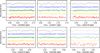 |
Fig. B.1 White light curves and the colour residuals against g, r, i, and z, light curves for six MuSCAT2 multi-colour light curves. One of the observed light curves is excluded due to poor photometric quality. |
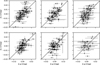 |
Fig. B.2 MuSCAT2 z- versus g-band light curves (in Δ mag). We do not detect any systematic colour signatures within uncertainties. |
All Tables
Difference in BIC (ΔBIC) relative to the best-fitting model for each TESS sector.
All Figures
|
Fig. 1 All i-band light curves ordered into groups and phase-folded to the 25.01 h period. The reference time for the phase folding is 2459928.85. The y-offset of the light curves in each group correspond to the 25.01 h period signal cycle. |
| In the text | |
|
Fig. 2 Multi-colour photometry from MuSCAT2, ProEM, and ALFOSC shown for filters g′ (blue), r (green), i, and i′ (yellow), and zs (red) and phase-folded to the 25.01 h period. The reference time for the phase folding is 0.0. The MusCAT2 photometry is binned to 3 min, the ProEM photometry to 2 min, and the ALFOSC photometry is not binned. The y-offset of the light curves corresponds to the 25.01 h period signal cycle. |
| In the text | |
|
Fig. 3 LS periodograms of the TESS photometry from Sectors 9, 36, 63, and 90. The known 23.1 min and 25.01 h periodicities are marked with solid orange and blue lines, respectively, while the 11.4 h signal is marked with a solid green line. The dashed and dotted lines indicate harmonics of these signals using the same colour-coding. |
| In the text | |
|
Fig. 4 GP periodograms for the long-period searches (3–29 h) from the TESS Sector 9, 36, 63, and 90 photometry. Left column: 1D periodograms for a single-period GP model. The plotted signal amplitude ΔBIC is defined as the difference between the BIC of the single-period GP model and that of the aperiodic GP model, i.e. ΔBIC = BIC1(p1) − BIC0. Right column: conditional 1D periodograms for a two-period GP model where p1 is fixed to 25.01 h. Here, ΔBIC = BIC2(p1 = 25.01 h, p2) − BIC1(p1 = 25.01 h). The known 25.01 h period and its harmonics are marked with solid and dashed blue lines, respectively, while the 11.4 h period and its harmonics are marked with the solid and dotted green lines. The horizontal slashed line shows the ΔBIC level of −10, which corresponds to very strong evidence in favour of the periodic signal (Kass & Raftery 1995). |
| In the text | |
|
Fig. 5 Posterior densities for the GP model hyperparameters estimated from the ground-based LCOGT observations and from separate TESS sectors. First column: GP coherence scale. Second column: GP harmonic complexity. Third column: amplitude of the periodicity. The 11.4 h period is estimated only from the TESS Sectors 9 and 36. The ground-based posterior estimates for the 25.01 h and 23.1 min periodicities are significantly better than the TESS ones due to the significantly higher photometric precision. |
| In the text | |
|
Fig. 6 Ground-based LCOGT observations for January and March 2024 (points with error bars) together with the GP model consisting of an aperiodic component, a 25.01 h quasi-periodic component, and a 23.1 min quasi-periodic component (black line) folded over the 25.01 h period. Top three panels: each separate GP component without the other components from the observations and the model. Bottom panel: observation residuals with respect to the full GP model. The cycle number is marked on the right, starting from the first light curve in the dataset. |
| In the text | |
|
Fig. 7 Posterior distribution of the ratio of the 25.01 h period and the 23.1 min period estimated from the 2 min cadence TESS photometry from the four TESS sectors. All sectors lie close to the 65:1 commensurability, except for Sector 36. |
| In the text | |
|
Fig. B.1 White light curves and the colour residuals against g, r, i, and z, light curves for six MuSCAT2 multi-colour light curves. One of the observed light curves is excluded due to poor photometric quality. |
| In the text | |
|
Fig. B.2 MuSCAT2 z- versus g-band light curves (in Δ mag). We do not detect any systematic colour signatures within uncertainties. |
| In the text | |
Current usage metrics show cumulative count of Article Views (full-text article views including HTML views, PDF and ePub downloads, according to the available data) and Abstracts Views on Vision4Press platform.
Data correspond to usage on the plateform after 2015. The current usage metrics is available 48-96 hours after online publication and is updated daily on week days.
Initial download of the metrics may take a while.