| Issue |
A&A
Volume 709, May 2026
|
|
|---|---|---|
| Article Number | A37 | |
| Number of page(s) | 39 | |
| Section | Extragalactic astronomy | |
| DOI | https://doi.org/10.1051/0004-6361/202557854 | |
| Published online | 01 May 2026 | |
BlazEr1: The eROSITA blazar catalog
Blazars and blazar candidates in the first eROSITA survey
1
Dr. Karl Remeis-Sternwarte and Erlangen Centre for Astroparticle Physics, Friedrich-Alexander Universität Erlangen-Nürnberg, Sternwartstr. 7, 96049 Bamberg, Germany
2
Department of Physics & McDonnell Center for the Space Sciences, Washington University in St. Louis, One Brookings Drive, St. Louis, MO 63130, USA
3
Department of Physics and Astronomy, Bowdoin College, Brunswick, ME 04011, USA
4
Deutsches Elektronen-Synchrotron DESY, Platanenallee 6, 15738 Zeuthen, Germany
5
Department of Physics and Astronomy, Clemson University, Clemson, SC 29631, USA
6
Max-Planck-Institut für extraterrestrische Physik, Gießenbachstraße 1, 85748 Garching, Germany
7
Max-Planck-Institut für Astronomie, Königstuhl 17, 69117 Heidelberg, Germany
8
INAF – Osservatorio Astronomico di Brera, Via E. Bianchi 46, 23807 Merate (LC), Italy
9
INAF – Osservatorio di Astrofisica e Scienza dello Spazio, via Gobetti 93/3, 40129 Bologna, Italy
10
Center for Astrophysics | Harvard & Smithsonian, 60 Garden Street, Cambridge, MA 02138, USA
11
Leibniz-Institut für Astrophysik Potsdam, An der Sternwarte 16, 14482 Potsdam, Germany
12
Institute of Astronomy, University of Cambridge, Madingley Road, Cambridge CB3 0HA, UK
13
Nicolaus Copernicus Astronomical Center, Polish Academy of Sciences, ul. Bartycka 18, 00-716 Warsaw, Poland
14
Julius-Maximilians-Universität Würzburg, Fakultät für Physik und Astronomie, Institut für Theoretische Physik und Astrophysik, Lehrstuhl für Astronomie, Emil-Fischer-Str. 31, 97074 Würzburg, Germany
15
Max-Planck-Institute for Radio Astronomy, Auf dem Hügel 69, 53121 Bonn, Germany
16
GFZ Helmholtz Centre for Geosciences, Telegrafenberg, 14476 Potsdam, Germany
17
NASA HQ, 300 E St. SW, DC 20546-0002 Washington, DC, USA
★ Corresponding author: This email address is being protected from spambots. You need JavaScript enabled to view it.
Received:
27
October
2025
Accepted:
4
March
2026
Abstract
Aims.eROSITA, on board the Spectrum Roentgen Gamma (SRG) spacecraft, performed its first X-ray all-sky survey (eRASS1) between December 2019 and June 2020. It detected about 930 000 sources, providing us with an unprecedented opportunity for a detailed blazar census properties of blazars and blazar candidates in eRASS1 and the compilation of the eROSITA blazar catalog.
Methods. We compiled a list of blazar and blazar candidates from the literature and matched it with the eRASS1 catalog, constructing the Blazars in eRASS1 (BlazEr1) catalog. For sources with more than 50 counts, we obtained their X-ray spectral properties. We compiled multiwavelength data from the radio to the γ-ray regimes for all sources, including multiwavelength spectral indices and redshifts. The full catalog is available online.
Results. We present the BlazEr1 catalog, containing 5865 sources, of which 2106 are associated with confirmed blazars. For 2966 sources, eROSITA provides the first X-ray data. The contamination from non-blazar sources of the entire sample is less than 11%. Most candidates exhibit properties typical for blazars. We present the properties of the entire X-ray detected blazar population, including the distributions of X-ray luminosities and photon indices, multiwavelength properties, and the blazar log N-log S distribution. Our catalog provides follow up targets, such as potential MeV and TeV blazars.
Conclusions. The BlazEr1 catalog provides a compilation of X-ray detected blazars and blazar candidates. The catalog serves as a starting point for exploiting further eROSITA surveys using the same methodology, enabling us to study the X-ray variability and a large number of spectral energy distributions of blazars in the future.
Key words: catalogs / surveys / galaxies: active / BL Lacertae objects: general / galaxies: jets / quasars: general
© The Authors 2026
 Open Access article, published by EDP Sciences, under the terms of the Creative Commons Attribution License (https://creativecommons.org/licenses/by/4.0), which permits unrestricted use, distribution, and reproduction in any medium, provided the original work is properly cited.
This article is published in open access under the Subscribe to Open model. This email address is being protected from spambots. You need JavaScript enabled to view it. to support open access publication.
1. Introduction
Active galactic nuclei (AGNs) with relativistic jets with a line-of-sight orientation toward Earth are referred to as blazars (Blandford & Rees 1978; Blandford & Königl 1979; Antonucci 1993; Urry & Padovani 1995; Schlickeiser 1996). Relativistic beaming makes blazars the most luminous persistent sources in the Universe and the dominant source type in X-ray and γ-ray wavelengths at high Galactic latitudes (Mattox et al. 1993), with high degrees of variability across the entire electromagnetic spectrum on timescales from minutes to years (e.g., Urry 1996; Tanihata et al. 2001; Ciaramella et al. 2004; Agarwal et al. 2015; Rajput et al. 2020).
Blazars emit a double-peaked multiwavelength spectral energy distribution (SED; see, e.g., Middei et al. 2022; their Fig. 1), which is often modeled by two log-parabola components (Massaro et al. 2006; Hinton & Hofmann 2009; Madejski & Sikora 2016; Krauß et al. 2016; and references therein). The low-energy peak originates from synchrotron emission of electrons (and possibly positrons) in the relativistic jets (e.g., Marscher & Gear 1985). The peak of this emission component is typically located between the radio and the optical bands (Fossati et al. 1998). In contrast, the high-energy component, with the highest level of emission in the γ rays, can be explained using leptonic, hadronic, or lepto-hadronic models (Böttcher et al. 2013). In the leptonic scenario, the jet is assumed to consist of electrons and positrons. Photons inverse Compton scatter off of the relativistic electrons and positrons in the jet to higher energies. The up-scattered photons could originate from the same population of synchrotron photons (synchrotron self-Compton radiation; SSC; Ginzburg & Syrovatskii 1965; Rees 1967; Jones et al. 1974; Maraschi et al. 1992; Dermer & Schlickeiser 1993; Bloom & Marscher 1996) or other photon fields, such as thermal emission from the accretion disk, the broad line region or the torus (external Compton; EC; Sikora et al. 1994; Ghisellini & Madau 1996; Finke 2016; and references therein). In hadronic models, the high-energy peak would be produced exclusively by relativistic protons (e.g., Mannheim & Biermann 1992; Mannheim 1993; Mücke & Protheroe 2001; Mücke et al. 2003), resulting in pions from proton-photon interactions. Neutral pions and their subsequent decay cascades then produce the observable X-ray and γ-ray photons (Liodakis & Petropoulou 2020). Leptonic and hadronic SED models are able to describe multiwavelength data adequately well due to degeneracies, incomplete multiwavelength coverage, nonsimultaneous data, and additional systematic uncertainties (e.g., Böttcher et al. 2013).
The spectral position of the peaks is a useful tool to classify blazars based on the energy of their synchrotron peak (Fossati et al. 1998; Abdo et al. 2010). Sources with low-energy peaks at νpeak ≤ 1014 Hz, above νpeak ≥ 1015 Hz, and in the intermediate range are called low (LSPs), high (HSPs), and intermediate peaked blazars (ISPs), respectively (Padovani & Giommi 1996). The X-ray band tends to fall in the energy range near the transition between the synchrotron and the high-energy peak. In a νFν representation, this results in a falling X-ray spectrum (Γ > 2.0) for a higher-peaked source, where the X-rays probe the synchrotron emission. A low-peaked source exhibits a rising (Γ < 2.0) X-ray spectrum, that is, X-rays are part of the high-energy peak (Blandford et al. 2019; and references therein). This basic classification with regard to the photon index from a single snap shot observation can be systematically affected by source variability, as during outburst and flares, sources can exhibit a peak-shift behavior, including possible extreme HSP behavior (e.g., Pian et al. 1998; Giommi et al. 2000; Ahnen et al. 2018; Sahu et al. 2021; Gokus et al. 2024b).
Blazars have historically been classified based on optical spectra: sources exhibiting emissions lines with widths of > 5 Å are called flat spectrum radio quasars (FSRQs, Stickel et al. 1991), while sources with weaker or even no emission lines are classified as BL Lacs (BLLs). In recent years, however, obvious weaknesses of the emission line classification scheme have been pointed out by multiple authors. Some sources clearly exhibit features of both classes, which led to the introduction of intermediate classes in some classification schemes (Turriziani et al. 2007), while other sources showed strong contributions from the host galaxy (BZG; Massaro et al. 2015). By studying a sample of 354 individual blazars with available multi-epoch spectroscopy, Ruan et al. (2014) found six cases of transition, attributed to the continuum of the jet sometimes outshining the emission lines, making these transitional objects likely FSRQs. As shown by D’Elia et al. (2015), especially for sources located at redshifts of z > 0.7, some emission lines that are redshifted into the infrared might be missed due to the lack of infrared coverage. From a sample of five sources classified as BLLs, as predicted by Giommi et al. (2012), D’Elia et al. found two sources which could be FSRQs, based on the line width. In addition, multiple changing-look blazars (i.e., sources transitioning between the FSRQ and BLL class) have been reported. These changes are believed to be related to changes in accretion rate (Kang et al. 2024).
In the context of the peak energy classification, FSRQs are predominately LSPs, while BLLs are distributed among all these different categories (Ghisellini et al. 1998). Overall, FSRQs are more bolometrically luminous (Ghisellini 2013). In fact, the position of the synchrotron peak is thought to be connected to the overall luminosity via the so-called “blazar sequence”. In other words, it might be that due to more efficient cooling the more luminous sources peak at shorter frequencies (Fossati et al. 1998; Ghisellini 2013). It is not clear, however, if this sequence is due to selection effects (see e.g., Giommi et al. 2012; Keenan et al. 2021).
To understand the population and the X-ray properties of blazars as a whole, it is necessary to systematically study a large sample. Blazars have been targets of many X-ray observations, mainly focused on bright or variable sources, due to the extensive multiwavelength campaigns required for SED modeling. Different X-ray observatories have been used to build X-ray catalogs. For these catalogs of known blazars, identified through optical, radio, and γ-ray surveys (e.g., catalogs compiled by, e.g., Massaro et al. 2015; Ackermann et al. 2015), were matched against the observational data. Samples obtained using only one observatory were built using Einstein (Worrall & Wilkes 1990, 55 sources), EXOSAT (Sambruna et al. 1994a,b; 26 sources), Beppo-SAX (Donato et al. 2005; 86 sources), ROSAT (Urry et al. 1996, 36 BLLs, Perlman et al. 1996b, 23 BLLs, Turriziani et al. 2007, 510 confirmed and 173 new blazars), Swift-XRT (Giommi et al. 2019; OUSXB1: 2308 sources), XMM-Newton (de la Calle Pérez et al. 2021; 103 sources), and NuSTAR (Middei et al. 2022; 126 sources). Other studies have used data from multiple X-ray missions (e.g., Comastri et al. 1997; Donato et al. 2001; Kadler 2005; Fan et al. 2012; Kapanadze 2013; Yuan & Fan 2014; > 500 sources), often aiming at the multiwavelength properties of blazars. All these catalogs only cover previously observed areas of the sky; therefore, these observations are often biased toward the preselected sources proposed as observation targets, which can introduce further biases in sky coverage. The few X-ray catalogs providing nearly all sky coverage suffer from limited flux sensitivity and the number of sources in these samples is therefore small compared to the number of blazars known in other bands.
A first X-ray sample with all-sky coverage and a deeper X-ray flux limit was obtained with the ROSAT all-sky survey (RASS; Truemper 1982, 1993; Voges et al. 1999, 2000). The newest RASS catalog (2RXS; Boller et al. 2016) offers information for roughly 135 000 sources with a limiting sensitivity of FX, 0.1 − 2.4 keV ∼ 10−13 erg cm−2 s−1 in the 0.1–2.4 keV band. Shortly after its publication, RASS was used to study the photon index distributions of blazars (Urry et al. 1996; Perlman et al. 1996b) and to derive blazar catalogs (e.g., Turriziani et al. 2007). For a long time, the RASS was the most comprehensive X-ray all-sky survey. This changed with the advent of the extended ROentgen Survey with an Imaging Telescope Array (eROSITA) on the Russian Spectrum-Roentgen-Gamma (SRG) satellite (Merloni et al. 2012; Sunyaev et al. 2021). Launched in July 2019 from Baikonur, the mission began all-sky-survey operations in December 2019 (Predehl et al. 2021; Merloni et al. 2024). Consisting of seven nearly identical Wolter type 1 X-ray telescopes, called telescope modules (TMs), with a total field of view of 1° and frame store CCDs in the focal plane, eROSITA is sensitive in the 0.2–10.0 keV band. eROSITA performed an all-sky slew survey as SRG, which orbits L2, constantly rotated around the spacecraft-Earth axis with a period of 4 h. Therefore, distinct positions on the sky were, on average, observed about six times in consecutive spacecraft rotations, while the source remained in the field of view for about 40 s during every visit. Close to the ecliptic poles, which coincide with the survey poles, the number of consecutive observations is a lot higher. Due to its L2-orbit and its rotation around the Sun the whole sky could be covered within half a year. Therefore, eROSITA allows us to observe the entire sky in a systematic, unbiased (unaffected by triggering on sources of interest) way and to investigate source variability on timescales of hours and months. In total, eROSITA observed the full sky four times as operations had to be halted for political reasons during the fifth all-sky scan in late February 2022. During the first all-sky scan by eROSITA (eRASS1), between December 2019 and June 2020, nearly 930 000 individual sources were detected on the Western Galactic hemisphere, which is accessible to the German eROSITA consortium (Merloni et al. 2024). This makes the eRASS1 catalog the largest X-ray source catalog to date. In the 0.5–2.0 keV band, 50% completeness across the entire sky is achieved at a flux of ≲5 × 10⁻¹⁵ erg cm−2 s−1. The vast majority of eRASS1 sources are AGNs (∼80%), enabling a census of accreting supermassive black holes of unprecedented completeness. eROSITA data therefore provide a great opportunity to investigate the X-ray properties of the blazar population. The first eROSITA all-sky survey has already been used to identify potential TeV blazars for follow-up (Marchesi et al. 2025; Metzger et al. 2025), to investigate neutrino events (Adriani et al. 2025), to identify high-redshift blazars (Wolf et al. 2024), and to study the intergalactic medium with blazars (Gatuzz et al. 2024).
We present the first eROSITA eRASS1 blazar catalog, including the X-ray identification and the X-ray and multiwavelength properties of blazars and blazar candidates found during eRASS1. In Sect. 2, we discuss the preparation of a sample of previously known blazars and blazar candidate sources, which is matched against the eRASS1 all-sky data. In Sect. 3, we describe our identification of blazars and the analyses of the eROSITA data. Additional multiwavelength data are discussed in Sect. 4. The properties of the blazars and blazar candidates observed by eROSITA are discussed in Sect. 5. We summarize results and provide future prospects in Sect. 6. Throughout the paper, we assume a flat Λ cold dark matter (ΛCDM) cosmology with ΩΛ = 0.7, Ωm = 0.3, and H0 = 70 km s−1 Mpc−1 (Beringer et al. 2012).
2. The BLAZE catalog: Catalog of blazars from the literature
As no recent standard catalog of blazars exists that includes all claimed or confirmed candidates in the literature, here we describe how we created a “master” catalog of blazars and blazar candidates by cross-matching existing catalogs from the literature. This catalog has been released at the time of this paper’s publication.
2.1. Construction of the catalog
Older blazar compilations, such as the 5th Roma-BZCAT catalog (Massaro et al. 2015; we refer to this catalog simply as BZCAT throughout the paper) miss a large number of newer sources. These catalogs are also significantly biased in terms of flux or region on the sky observed (e.g., Bellenghi et al. 2023). To search for X-ray counterparts of known blazars, we constructed a catalog of blazar and blazar candidates from catalogs found in the literature. As many sources are included in multiple catalogs, we filtered for duplicates by positional matching, taking into account the accuracy of the individual catalogs. The catalogs used to build the “master” list, the number of sources provided by the catalogs and the number of sources added, and the radii used to identify duplicates with respect to other catalogs and the spectral classes provided, are listed in Table 1.
Blazar and blazar candidate catalogs used to build the BLAZE catalog.
Following, for instance, Giommi et al. (2019) and Bellenghi et al. (2023), we combined all the blazars and blazar candidates from the latest data release of the fourth Fermi-LAT source catalog (4FGL-DR4; Abdollahi et al. 2020, 2022), the BZCAT multi-frequency catalog (Massaro et al. 2015), and the 3HSP catalog (Chang et al. 2019). For the source positions of the Fermi-LAT blazars, we used the coordinates of the associated counterparts provided in the 4FGL catalog, since the γ-ray positions were not well constrained enough. Duplicates were identified by position matching or using associations provided by the input catalogs. Since the catalogs have different spatial accuracy, each catalog was assigned an individually selected maximum radius within which the sources were considered duplicates (see Table 1). In addition, we added 48 high-redshift blazars reported in the literature (Yuan et al. 2000, 2003; Sowards-Emmerd et al. 2003; Romani et al. 2004; Worsley et al. 2004; Shemmer et al. 2006; Healey et al. 2008; Sbarrato et al. 2012, 2013, 2015, 2022; Ghisellini et al. 2014, 2015b,a; Massaro et al. 2015; Coppejans et al. 2016; Belladitta et al. 2019, 2020; Caccianiga et al. 2019; Ighina et al. 2019; Khorunzhev et al. 2021; An et al. 2023; Marcotulli et al. 2025). This sample of high-redshift sources was compiled by Sbarrato et al. (2026)2 and extended by us with the source discussed by Marcotulli et al. (2025). This sample will be referred to as the HighZ sample.
In addition to sources with a confirmed blazar designation, we added objects with properties that are similar to those of blazars, with varying criteria depending on the input catalog. We started with the Milliquas catalog (Version 8, Flesch 2023). This catalog contains mainly AGNs but also lists BL Lac-like objects identified via various detection methods. Based on WISE data, the KDEBLLACS and WIBRaLS2 catalogs provide candidate blazars of various spectral types (D’Abrusco et al. 2019), while the ABC catalog (Paggi et al. 2020) uses ALMA calibration data as well as other multiwavelength information to characterize blazar candidates. The largest catalog used to build our candidate sample is the BROS catalog (Itoh et al. 2020). This catalog lists objects which exhibit a flat radio spectrum and a counterpart in Pan-STARRS1. Compared to other catalogs, BROS sources are not homogeneously spread across the entire sky, but cover areas with Galactic latitude |b|≥10° and declination δ > −40°. A small window centered around Galactic coordinates b ∼ 40° and l ∼ 220° was excluded due to a lack of radio coverage. To create the master list, we started with the first catalog shown in Table 1, then cross-matched with the next catalog and added any previously not included sources. We continued this process down the list of catalogs given in Table 1.
Our initial list after positional cross-matching contained 103 498 individual blazars and blazar candidates spread over the entire sky, of which 43 148 (∼41%) are located on the western Galactic hemisphere due to the inhomogeneity of the BROS catalog. Based on the input catalogs, we classified the blazars and blazar candidates into the following classes: (1) a BL Lac object is listed as BLL; (2) a galaxy-dominated BL Lac object is denoted as BZG; (3) a flat spectrum radio quasars is abbreviated as FSRQ; and (4) a confirmed blazar of an unknown type is called BCU. We appended the letter “C” to the abbreviation to indicate that a source is a blazar candidate (BLLC, BCUC, FSRQC). If no spectral classification is listed, sources were denoted as BCUC, which included all entries originating from the BROS catalog. The classifications from the input catalogs for BLLs and FSRQs, and of course the corresponding candidates, have to be taken with caution, since roughly 2–5% of these sources are probably misclassified (Ruan et al. 2014; D’Elia et al. 2015; Kang et al. 2024). Therefore, we estimate that at most 180 confirmed BLLs and FSRQs and 560 corresponding candidates are wrongly grouped in the initial list. An extensive and detailed spectroscopic study would be needed to further investigate the correct classification of sources on the list, which is beyond the scope of this study.
2.2. Assessment of quality
No source in the initial master list is guaranteed to be a blazar, especially since there are many candidates. Thus, it is important to assess the contamination and remove as many non-blazars as possible.
Due to the extremely complex selection function, assessing the contamination is not straightforward. We therefore investigated a few indicators and assigned upper limits to the level of contamination and checked the purity of the input catalogs. In the 4FGL, about 98% of AGNs are confidently classified as blazars and, hence, we would expect a very low level of contamination. A similar level of purity is expected from BZCAT; however, this catalog also contains radio galaxies such as Cen A. According to Xie et al. (2024) about 5% of BZCAT sources are non-blazars. The 3HSP contamination is expected to be < 2% (Chang et al. 2019) and similar levels are expected from the HighZ sample. Unfortunately, no level of contamination is listed for the sample of the Milliquas and the ABC. de Menezes et al. (2019) assessed the contamination of the WIBRaLS2 and KDEBLLACS catalogs using SDSS. They found that 31% and 30%, respectively for these catalogs, are blazars. The main contamination is caused by QSOs (∼69%), which could also be blazars, representing a loosely constrained upper limit. These catalogs were also tested by Xie et al. (2024). They find 14% and 12% to be non-blazars, respectively. The difference between the estimated levels of contamination for the WISE catalogs might be related to the entire sample not having available data in both approaches and due to other thresholds set to distinguish a blazar from a non-blazar. For the BROS catalog, Itoh et al. (2020) estimated a contamination of about 10%. Due to flux and spatial limits in the BROS data, only 60% of the BZCAT sources are also present in this catalog. Therefore, we expected roughly 5% of the blazars and about 14% of the candidates listed in the master list to be non-blazars, when utilizing the most conservative estimates presented above.
To identify non-blazar contamination by nearby galaxies in our list (and since blazars have higher redshifts), we matched against the HECATE catalog of nearby galaxies (Kovlakas et al. 2021), one of the most complete catalogs of galaxies in the local Universe (D ≲ 200 Mpc) at the time of writing. We obtained 1227 matches within 12″ of the galaxy center, of which 1215 are located within the D25-ellipse. Out of these, 57 positional matches are associated with confirmed blazars, including well known sources with redshifts consistent with the matched HECATE galaxy; hence, it is clear that the position alone is not enough to identify non-blazars. HECATE also offers a Hubble galaxy classification (de Vaucouleurs et al. 1976). Out of the positional matches 689 correspond to a spiral galaxy. Since blazars are typically not hosted in spiral galaxies (Urry et al. 2000; O’Dowd et al. 2002) and a location within the D25-ellipse with a maximum separation of 12″ indicates that in X-rays the source is undistinguishable from the center of the Galaxy, we excluded these 689 objects, almost 99% of which originate from the BROS catalog.
Xie et al. (2024) used moderate resolution radio images from the VLA Sky Survey (VLASS; Lacy et al. 2020) to classify the sources from BZCAT, WIBRaLS2, and KDEBLLACS based on their morphology. We matched the initial list with their results using the match radii for the individual catalogs (see Table 1). If a visual assessment of the morphology exists we used this classification instead of the automated one. A two-sided radio morphology, which is inconsistent with the source being classified as a blazar, was found for 1139 objects. These outliers were then removed.
Due to their different optical and X-ray spectra, as well as due to their typical radio-quietness, we removed known narrow-line Seyfert 1 (NLSy1) galaxies, even though a fraction of the NLSy1 galaxy population has been detected in the radio band (e.g., Komossa et al. 2006; Singh & Chand 2018), with a small number also having been detected at γ rays (e.g., Abdo et al. 2009; Paliya et al. 2018). Several authors have shown that γ-loud NLSy1s exhibit blazar-like characteristics including bright flaring episodes (e.g., D’Ammando et al. 2015; Paliya & Stalin 2016; Gokus et al. 2021), but ended up arriving at the conclusion that these objects resemble less powerful (i.e., younger sources). We excluded γ-ray emitting NLSy1 galaxies from the initial list to consider only “full-scale” blazars. Two NLSy1s listed in the 4FGL are located on the western Galactic hemisphere and detected by eROSITA (1eRASS J094857.1+002226 and 1eRASS J200754.9−443446). To exclude NLSy1s which do not show γ-ray emission, we matched with the catalog of NLSy1 galaxies by Rakshit et al. (2017). We found 55 matches within 5″ of initial list sources, the maximum match radius used during the construction of the master list, of which 37 were associated with candidates that were also removed.
To identify other types of radio galaxies, we matched against the high-fidelity sample from Gordon et al. (2023), made up of double radio sources, which is a morphology not expected to be observed for blazars. We again used a maximum separation of 5″, identifying 1243 matches. More than 76% of them were associated with a BROS source and overall 96.4% of the matches were blazar candidates. We also removed these.
Finally, we removed individual objects which are known to be non-blazars. BROS J0729.1+2054 is the counterpart of the Galactic planetary nebula NGC 2392. The nature of the source 4FGL J0647.7−4418 is debated in the literature either as being a blazar (Martí et al. 2020) or a B-type subdwarf and white dwarf binary (HD 49798; Mereghetti et al. 2009; Rigoselli et al. 2023). The young radio galaxy PMN J1603−4904 (Müller et al. 2015; Krauß et al. 2018) is falsely classified in 4FGL as the blazar 4FGL J1603.8−4903. Finally, the BZCAT catalog erroneously includes the radio galaxy Cen A as a blazar (5BZU J1325−4301).
2.3. Release and comparison with other catalogs
After removing obvious non-blazars, 100 368 out of the initial 103 498 objects remained. We call our master list of blazars and blazar candidates the BLAZars from litErature catalog, or BLAZE catalog. The BLAZE catalog can be split into a “gold sample”, which includes 6301 confirmed blazars with or without a known type (3031 are located on the footprint of the eRASS1 survey), and a “silver sample” of 94 067 candidates (38 905 in the footprint of the eRASS1 survey), containing the blazar candidates. Figure 1 shows the spatial distribution of the gold sample. Due to the general utility of a compilation of blazars for the field, the BLAZE catalog was published with this paper and made available online on Vizier. The description of the BLAZE catalog is given in Appendix C, as the catalog is enriched with redshifts for the confirmed blazars and eROSITA exposure times and upper limits for flux and luminosity. The list of the likely non-blazar objects, referred to as the ”unverified” BLAZE catalog, has been released as a separate file. Because the BLAZE catalog was compiled from multiple input catalogs with different wavelength selections and flux limits, and because obvious non-blazars sources were removed introducing new selection cuts, the population of blazars and blazar candidates listed in BLAZE is neither complete nor statistically well defined. Extensive simulations would be required to assess the completeness and the flux limits in different bands for the BLAZE catalog, which is beyond the scope of this study.
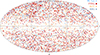 |
Fig. 1. All-sky distribution of the BLAZE catalog gold sample (confirmed blazars) in Galactic coordinates (BLL: 1697, FSRQ: 1937, BCU: 2503, BZG: 164). The different blazar classes are shown color coded and with different symbols. |
In comparison to previous studies, we found 6307 individual blazars from the 4FGL, BZCAT, and 3HSP catalogs; this is a slightly different number than in earlier catalogs (5340 sources, Giommi et al. 2019 and 6425 sources, Bellenghi et al. 2023). To avoid source confusion, we applied a stricter angular limit for cross-matching, leading to a difference between BLAZE and Giommi et al. (2019) and Bellenghi et al. (2023). The deviation of 15% between BLAZE and Giommi et al. (2019) is also related to this estimate being based on the 3LAC catalog which only contains 1591 sources in total compared to the 3934 included in the 4FGL catalog. However, the deviation between the BLAZE and Bellenghi et al. (2023) is only 2% mainly driven by the exclusion of contaminants. Marchesi et al. (2025) found 1772 matches between the BZCAT and the 4FGL, of which 1725 are within 2″, while our analysis returns 1625 within 4″ (1731 without quality cuts). This difference is ascribed to our match radius, as Marchesi et al. (2025) also accept wider separations for counterparts between the catalogs and our filtering. A total of 615 out of 651 objects in the isotropic catalog of Kudenko & Troitsky (2024) are contained in the BLAZE catalog, which includes 409 of the 433 blazars and blazar-like sources from the isotropic catalog. The objects not contained simply do not have a counterpart in Kudenko & Troitsky (2024, to within 6′). Out of the matches, 204 are classified as quasars, AGNs or based on an emission band by Kudenko & Troitsky (2024) and 19 of these are associated with blazar candidates in the BLAZE catalog. A radio flux-limited sample of HSP sources was constructed by Giommi et al. (2020) based on Puccetti et al. (2011). Of the 23 sources in this sample, 15 are included in the BLAZE catalog, including all sources associated with the 3HSP catalog. Again, this stresses that the BLAZE catalog, although it is the largest catalog to date, is not complete.
3. Matching eROSITA to the BLAZE catalog
In this section, we describe the construction of our eROSITA blazar and blazar candidates catalog based on the BLAZE catalog. Out of the 100 368 blazar and blazar candidate sources in the BLAZE catalog, 41 936 are located on the western Galactic hemisphere and were matched with eROSITA. We also assess the level of contamination of the catalog and the analysis of the X-ray data.
3.1. The eROSITA observed blazars and blazar candidates
3.1.1. X-Ray counterparts
To identify the X-ray counterparts of the BLAZE catalog, we matched the BLAZE catalog and the eRASS1 catalog positions (Merloni et al. 2024). We used the BLAZE catalog and the attitude-corrected positions from eROSITA, only considering point sources (EXT = 0.0, see Merloni et al. 2024) and identified an initial number of 8117 matches with angular separation ≤15″. This separation limit is based on the accuracy of the astrometric correction of eROSITA (Merloni et al. 2024) and the point spread function of the eROSITA telescopes. The histogram of the angular distance in Fig. 2 shows that most matches are within the positional accuracy of the matched eROSITA sources (shown in yellow, the normalized version of the histogram is displayed in Fig. A.1). About 84% of associations have an angular separation of 8″ or less, and 38% and 64% of the sample are located within 3″ and 5″, respectively. The distributions of separations for blazars and blazar candidates are different; the candidates exhibit a broader peak, possibly due to contamination. Based on the distribution of angular separation and to avoid unnecessary source confusion and false identifications we conservatively cut our final sample at a separation of 8″ between the BLAZE and eRASS1 source position. This cut reduced the sample to 6852 blazars and blazar candidates.
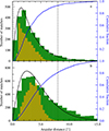 |
Fig. 2. Histograms of angular separation between BLAZE catalog and eROSITA positions (green) with the distribution of the matched eROSITA source positional uncertainty overlaid (yellow). The vertical line at 8″ indicates the distance threshold for the final sample. The cumulative distribution of the angular separation is shown in blue. a Sample of eROSITA observed blazars with 93% of the matches found within 8″, and 55% and 79% within 3″ and 5″, respectively. b eROSITA observed blazar candidates. Only 81% of matches are within 8″, and 31%/58% within 3″/5″. We show Rayleigh distributions (black) for illustrative purposes, calculated following Merloni et al. (2024, Eq. (3), assuming F = 0.8). |
Since the eROSITA exposures were still quite low (∼240 s), many sources have a low detection likelihood in eROSITA. To avoid including possibly spurious detections, we removed all matches with a detection likelihood, DET_LIKE_0 < 103, which reduces the fraction of spurious sources to ∼1% (Seppi et al. 2022; Merloni et al. 2024). We also removed all entries with uncertain positions, that is, those without values for RA_LOWERR, RA_UPERR, DEC_LOWERR, and DEC_UPERR in the eRASS1 catalog, and excluded all objects where eROSITA quality flags indicate issues in the source detection (FLAG_SP_SNR, FLAG_SP_BPS, FLAG_SP_SCL, FLAG_SP_LGA, FLAG_SP_GC_CONS, FLAG_NO_RADEC_ERR, FLAG_NO_CTS_ERR, and FLAG_NO_EXT_ERR). Additionally, we removed all blazars and blazar candidates with X-ray luminosities too low to actually be a blazar (LX, 0.2 − 2.3 keV < 1041 erg s−1), lowering our contamination rate. This reduced the sample size to 5865 sources of which 2106 are associated with confirmed blazars, and the remainder with blazar candidates. The normalized separation distributions shown in Fig. A.1 clearly indicate that after the applied cuts the agreement with the theoretical Rayleigh distribution is significantly improved. Table 2 lists the number of sources after each cut and for each blazar type, and Fig. 3 displays the sky distribution of the final sample.
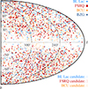 |
Fig. 3. Positions of the BlazEr1 sources in Galactic coordinates. The different colors and symbols indicate the blazar types in the catalog. Candidates, especially BCUCs, dominate the sample. The overdensity along l ∼ 240° coincides with the footprint of BROS. Confirmed blazars are displayed by filled symbols, candidates are shown in the same color without filling. All the following figures will adapt the same color and symbol scheme. |
Breakdown of the blazar source classes during the construction of the BlazEr1 catalog.
The matches outlined above are the basis for the Blazars in eRASS1 (BlazEr1) catalog. This catalog combines X-ray and multiwavelength information that we compiled for all catalog sources. A detailed description of the content of the catalogs is given in Appendix D. We refer to the sample of sources detected by eROSITA and associated with “gold sample” BLAZE sources as “eROSITA observed blazars”, while we refer to the eROSITA matches with an entry from the BLAZE “silver sample” as “eROSITA observed blazar candidates”. The 2252 objects removed from the catalog are included in a separate catalog, as this sample is expected to be less pure, but it might still be of value for follow-up studies. Due to the survey mode of eROSITA, we are able to obtain a view unbiased by variability or source luminosity, and only limited by eROSITA sensitivity variations and exposure in eRASS1.
3.1.2. Validation of positional matching
Since our association of blazars with eROSITA sources is based on positions, it was necessary to check whether our positional matching is a valid approach. We used two independent methods to derive an upper limit on the possible contamination of matching by pure chance.
We first estimated the possibility of randomly associating an input position with an eRASS1 source by uniformly distributing 5 × 10⁵ (which is five times larger but has the same order of magnitude in numbers as the BLAZE catalog) sources at random position on the entire sky and matching these positions to the eRASS1 catalog. Within 8″, we found 346 matches whereas within 15″ 1205 matches were found, indicating a probability for random association of 0.07% and 0.24% for these separations, respectively. Alternatively, conserving the density properties of the eRASS1 survey we rotated the positions in the eRASS1 catalog around the ecliptic poles by a few degrees in ecliptic longitude and then matched them with the BLAZE catalog. For rotations by 1° and 10°, 89 and 104 sources matched within 15″, respectively. When reducing the separation to 8″, only 34 and 23 matches remained, implying a random match probability of about 0.08% for a separation of < 8″, regardless of the applied rotation.
Results from both methods suggest a probability below 0.1% of accidental source confusion. Hence, we expect at most 42 eROSITA detections to be randomly assigned to BLAZE catalog sources. Given the size of the BlazEr1 catalog, the rate of source confusion is therefore at a negligible level of 0.7%. Our cross-matching angular distance is well justified, as the loss of matches when reducing the acceptable angular distance from 15″ to 8″ indicates that the probability of including random matches drops significantly. We emphasize that this low level of accidental source confusion is due to us using pre-existing positions of objects with known multiwavelength properties, including a very high probability that these sources are X-ray bright. This approach is different from approaches that attempt to find multiwavelength counterparts for new X-ray detected sources in multiwavelength catalogs, where little is known about the properties. These approaches have a much higher probability of misidentifying the multiwavelength counterparts.
3.2. Contamination
The sample size makes a study of the source nature on an individual basis too time consuming. Therefore, we try to asses upper limits of the contamination. We derived the level of contamination caused by non-blazars in the sample by comparing the BlazEr1 catalog with the catalog of Legacy Survey data release 10 (LS10; Dey et al. 2019) counterparts of eRASS1 point sources (Salvato et al. 2025; hereafter S25). This catalog is based on an identification of optical counterparts with the Bayesian algorithm NWAY (Salvato et al. 2018), using a combination of astrometric information such as separation, positional error, and source number density (similar to Xmatch; Pineau et al. 2017). The completeness and purity of the LS10 catalog of counterparts to eRASS1 is ∼93% (S25).
We matched by using the detection ID of eRASS1. If more than one possible counterpart was listed for a given ID, we used the one with the closest position. In total, we can match 84% of the BlazEr1 sources (4924 objects). We only considered counterparts to be a match between both catalogs if the association of S25 and the BlazEr1 catalog have an angular separation of at most 2″, and if pany ≥ 0.14. For 508 matches (10.3% of the sources with a match based on detection ID) we associated a different counterpart as S25 or pany is very low. About 89% of the disagreed upon objects are associated with blazar candidates and almost 80% originate from the BROS catalog. This leaves us with 4416 counterparts in common, which corresponds to a 90% agreement. Therefore, when comparing with the results of S25 and assuming that their assigned counterparts to the eROSITA sources are all correct, a disagreement between the counterpart by S25 and our catalog and hence a contamination of at maximum 3.3% for the eROSITA observed blazars and 14.0% for the eROSITA observed blazar candidates is expected. Sometimes the X-ray source might be the sum of multiple emitters. This is the case for 32 sources, of which in 22 cases the counterparts by S25 and our source are identical. We also compared the matches obtained by matching the unverified BLAZE catalog with eRASS1, using the same methodology as for the BlazEr1 sample, with the counterpart catalog. Given the same criteria as listed in Sect. 3.1, the unverified BLAZE catalog has 491 matches with the eRASS1, of which 397 have a counterpart in S25. For 33 of these matches, all of them candidates, S25 assigns a different counterpart. Therefore, a slightly lower (but similar) level (∼8%) of contamination has been reached for this low-quality sample as for the BlazEr1 catalog. This also indicates that cleaning of the BLAZE catalog is useful.
For all eROSITA sources listed in the BlazEr1 and the counterpart catalog, we compared the angular separation between the eROSITA position and the counterpart by S25 with the separation between the BLAZE catalog source and eROSITA, normalized by the positional uncertainty of eROSITA. Some BlazEr1 counterparts tend to be too far away as they lie significantly above the theoretical Rayleigh distribution, whereas few counterparts assigned by S25 seem to be closer or more distant than expected (see Fig. A.2). This indicates that some BLAZE catalog objects are erroneously associated to the eROSITA source or that some of the associations of S25 might not be the correct counterpart. The estimated number of contaminating sources based on the assumption that S25 provides the correct counterpart and disagreement indicates contamination therefore represents an upper limit. We also note that ours and Salvato et al.’s counterpart associations methodologies differ significantly. While we focus on selecting blazar specific objects using multiwavelength information and pre-existing catalogs, the approach from Salvato et al. has been finetuned toward general X-ray emitters, where non-jetted AGNs dominate the population of X-ray emitting extragalactic objects. However, an in-depth comparison between the approaches is beyond the scope of this paper.
The contamination is mainly driven by the BLAZE catalog selection function and not by random matches (see Sect. 3.1.2). The most pessimistic estimates from the purities of the input catalogs (see Sect. 2.2) and the comparisons with the counterpart catalog indicate that the contamination for confirmed blazars is at most 5%, and ∼14% for the candidate blazars. The limit for the confirmed blazars is based on the purity estimate of the BZCAT by Xie et al. (2024), which has the highest impurity of the confirmed blazar catalogs. Although sources are excluded from the BLAZE catalog based on Xie et al. (2024), they do not provide a classification for all catalog entries. We therefore expect the subsample not covered by Xie et al. (2024) in the BZCAT to have a similar level of contamination as the overall catalog, and since we do not have information available for all BZCAT objects we adapt the 5% limit as an upper limit for the entire sample of confirmed blazars. For the candidates the limit is based on the contamination estimate based on the comparison with S25. Therefore, at most 106 of the thought to be confirmed blazars and 527 of the candidates are non-blazars. In total, less than 11% of the BlazEr1 catalog is contaminated, corresponding to a purity of almost 90%.
3.3. Survey sensitivity
Since the sensitivity of the eROSITA survey is not uniform across the sky, it is crucial to determine the lowest flux sources that could have been detected as a function of position and exposure time. We used the official eROSITA mission simulator, SIXTE (Dauser et al. 2019) to determine this sensitivity limit. Using the as-flown eROSITA attitude of the first all-sky survey and a diffuse foreground from ROSAT, we simulated eROSITA observations of 105 sources randomly and uniformly distributed across the western Galactic hemisphere. Based on the expected blazar spectrum averaged across the entire population, each source was assigned an absorbed power law spectrum (ΓX = 2.0, NH = 1 × 1021 cm−2). We varied the 0.2–2.3 keV flux between 1 × 10⁻¹⁶ and 1 × 10⁻¹¹ erg cm−2 s−1, with 20 000 random flux values per flux decade. The simulated data were then sorted into event lists for each eROSITA sky tile and processed using the official source detection pipeline contained in the eROSITA data analysis software eSASS (version 211 214, Predehl et al. 2021; Brunner et al. 2022; Merloni et al. 2024). The processing yielded a mock catalog containing information on the detection likelihood, exposure times, and fluxes. To ensure the validity of the simulations, we checked that all fluxes of the detected source are consistent with the input values within uncertainties; and since this is the case we used the input fluxes.
To estimate the completeness and sensitivity, we defined the survey as complete if, for a given exposure time and minimum detection likelihood of 10, 95% of sources with a given flux were detected. For a given minimum detection likelihood, we found that we can approximate the minimum detectable flux by
 (1)
(1)
where for the given minimum DET_LIKE_0 = 10, Isens = 2.14 × 10⁻⁹ erg cm−2 s−1, t0 = −13.90 s, Γsens = 2.20, and F0 = 2.02 × 10⁻¹⁴ erg cm−2 s−1. Combining Eq. (1) with the eROSITA exposure map, we were able to determine the area of the sky at which the survey is sensitive to a specific flux. We divided the sky into equally-sized pixels with an area of 0.002 deg2 and determined the minimum flux within that pixel. Figure 4 shows that the survey is complete on the whole western sky down to a flux of FX, 0.2 − 2.3 keV ∼ 2 × 10⁻¹³ erg cm−2 s−1. For all sources with a lower flux, corrections using the derived sensitivity will have to be applied, for instance when deriving log N-log S-distributions.
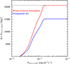 |
Fig. 4. Sky area in which 95% of all sources above a minimum flux will be detected with DET_LIKE_0 ≥10. The dashed line indicates the total area of the western Galactic hemisphere. The red line displays the sensitivity over the entire western Galactic hemisphere, while the blue line shows the extragalactic sky excluding an area of 15° below and above the Galactic plane and regions with radii of 5.5° around the Large Magellanic cloud (LMC) and 3.0° around the Small Magellanic cloud (SMC). |
3.4. X-ray spectral analysis
In order to gather information on the X-ray properties of our sample, we complemented the available eRASS1 catalog data (Merloni et al. 2024) with spectral information, using eSASS version 211 214, HEASOFT version 6.30, and eROSITA event processing version 020, which offers improved calibration compared to the release version 010 used by Merloni et al. (2024). While the processing version affects the quality of spectral products, it does not affect the source detection itself within the conservative selection criteria applied above. Tests with different processing versions revealed that their influence on the overall spectral fitting results does not change the overall results. We extracted source spectra from circular extraction regions centered on each catalog source, scaling the extraction region radius, R, on the maximum likelihood count rate for the 0.2–2.3 keV band, given by Merloni et al. (2024),
![Mathematical equation: $$ \begin{aligned} R = N \times (\mathrm ML\_RATE\_1 \,[\mathrm{cts} /\mathrm{s} ])^\gamma \end{aligned} $$](/articles/aa/full_html/2026/05/aa57854-25/aa57854-25-eq2.gif) (2)
(2)
where  and γ = 0.284. Higher count rate sources required larger regions to include all source photons, however we required at least 23″ and at maximum a region with a radius of 200″. Background regions are annuli centered on the source position, using Eq. (2) to scale the inner and outer radius. Specifically, for the inner radius we set
  , γ = 0.242, Rinner, min = 54″, and Rinner, max = 350″. For the outer radius,
  , γ = 0.282, Router, min = 280″, and Router, max = 2200″. Within the background region we excluded all neighboring eRASS1 sources, scaling the exclusion radius of each source by their count rate. Spectra were then extracted from event lists with the eSASS task srctool. Since eROSITA TM 5 and 7 are affected by light leaks (Predehl et al. 2021; Merloni et al. 2024), these two modules required special treatment in our analysis. Unless mentioned otherwise, for these TMs, only data taken > 1 keV were considered. For the spectral analysis, we used the Interactive Spectral Interpretation System (ISIS, version 1.6.2; Houck & Denicola 2000) and quote all uncertainties at 90% confidence for one independent parameter, unless stated otherwise.
For all sources, we collected basic source information such as the total amount of source counts and on-axis exposure times. The count information is given as the number of photons detected by all TMs for the 0.2–2.3 keV band, or as the combination of counts measured between 1.0–10.0 keV for TMs 5 and 7 and 0.2–10.0 keV for all other TMs. We utilized the Bayesian approach of Park et al. (2006) to determine hardness ratios,
 (3)
(3)
where NSo and NHa are the counts in the softer and harder band, respectively, and their uncertainties. We ignored TMs 5 and 7, and used the energy bands 0.2–0.7 keV, 0.7–1.2 keV, and 1.2–5.0 keV, hereafter bands 1, 2, and 3. For an absorbed power law with NH = 1 × 1021 cm−2 and photon index ΓX = 2, these bands contain a similar number of photons. The different hardness ratios are designated as follows: HR12 is the hardness calculated using bands 1 and 2, HR23 uses bands 2 and 3, and HR13 bands 1 and 3. The uncertainties given for the hardness ratios correspond to the smallest credible interval at 90% confidence around the most likely value.
The source fluxes reported in the eRASS1 catalogs were determined as part of the eROSITA source detection pipeline. They are based on maximum likelihood methods, applying predetermined energy conversion factors assuming an absorbed power law with ΓX = 2.0 and an absorption column density of NH = 3 × 1020 cm−2. We determined source intrinsic fluxes for the 0.2–2.3 keV band based on spectral modeling with fixed parameters. We used simple absorbed power laws tbabs*powerlaw (tbabs(1)*powerlaw(1)"), with the abundances of Wilms et al. (2000) and the cross-sections of Verner et al. (1996) and fix the equivalent hydrogen column, NH, to the 21 cm value for the source position reported by the HI4PI Collaboration (2016). We then determined the 0.2–2.3 keV fluxes from fits of the spectral continuum to the full eROSITA energy range from 0.2 keV (1 keV for TM5 and 7) to 10.0 keV for four fixed photon indices, ΓX, covering the range expected from blazar-like spectra ΓX = {1.5, 1.7, 2.0, 2.3}.
For the 1273 sources with more than 50 counts detected in the 0.2–2.3 keV band, we also performed a more detailed spectral analysis, again using an absorbed power law. For these, we dynamically rebined each spectrum following Kaastra & Bleeker (2016), while requiring that each bin contained at least one count, left the photon index free, and fixed NH to the 21 cm value from the HI4PI Collaboration (2016). Spectral minimization is based on Cash statistics (Cash 1979; Kaastra 2017). Figure 5 shows the spectra of three blazars with our best fit model. The fluxes derived from the fixed photon index power law fits, those determined during the spectral fits, and the ones reported by Merloni et al. (2024) are all similar within ∼18%. For high fluxes (≥FX, 0.2 − 2.3 keV ∼ 10−11 erg cm−2 s−1; Merloni et al. 2024) eROSITA spectra are influenced by pileup (see, e.g., König et al. 2022); we proceeded to check for pile-up in these sources. Using SIXTE to simulate blazar-like spectra within different flux ranges (also above the flux limit reported by Merloni et al. 2024) we found that our spectra are not significantly affected by pileup, with a maximum pileup fraction of 1.79% for the brightest source.
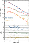 |
Fig. 5. Spectral fits of an absorbed power law model for three confirmed blazars with different fluxes. For 5BZQ J0547−6728, no prior X-ray observations are available. The three lower panels display the fit residuals for each source. Data from TM5 and 7 are displayed in a lighter color. |
4. Additional multiwavelength data
To put the properties of the BlazEr1 catalog into the multiwavelength context of these sources, we supplemented the eROSITA information with data from other X-ray and multiwavelength catalogs.
4.1. Observations of eROSITA blazars with other X-ray missions
To collect soft X-ray flux and spectral information, we cross-matched the BlazEr1 with the ROSAT (0.1–2.4 keV, Boller et al. 2016) and the Swift-XRT (0.3–10.0 keV) source catalogs by Giommi et al. (2019, OUSXB DR3) and Evans et al. (2020). Although both catalogs use Swift-XRT, they were compiled independently and using different approaches. The OUSXB catalog specifically targets blazars and treats each single observation separately; whereas Evans et al. (2020) merge all exposures of a given target. BlazEr1 counterparts are again identified by positional cross-matching, using a maximum angular separation between the BlazEr1 position and ROSAT of 40″ and of 8″ between BlazEr1 and Swift-XRT. We find 1496 ROSAT and 1249 Swift-XRT (for Evans et al. 2020) counterparts. As the OUSXB catalog is built on an observation basis with one entry per observation, we first matched it with the BLAZE catalog. For each of the 1039 matches we then derived the mean, median, minimum, and maximum fluxes and spectral indices from all source visits.
In order to get information at higher energies, we cross-matched the BlazEr1 with the NuSTAR (3.0–10.0 keV, 10.0–30.0 keV) blazar catalog (Middei et al. 2022), using a maximum angular separation of 8″ (based on the positional accuracy of NuSTAR; Harrison et al. 2013), identifying 46 out of 126 sources. Since this catalog contains one entry per observation, we included the fluxes and spectral information of the observation closest in time to eRASS1 to the BlazEr1 catalog. We also matched our detections with the Swift-BAT catalog (14.0–195.0 keV, Lien et al. 2025), assuming a maximum angular separation of 60″, and where available using the positions of already known counterparts, obtaining 96 matches, for which we added the flux and spectral information to the BlazEr1.
To identify objects with previous observations, we cross-matched BlazEr1 with the observation catalogs of XMM-Newton, Chandra, ASCA, NuSTAR, Suzaku, Swift-XRT, and ROSAT available at HEASARC5. BlazEr1 contains the total exposure time for each source and mission until the end of the eRASS1 survey.
4.2. The γ-ray counterparts of eROSITA blazars
The Large Area Telescope (LAT; Atwood et al. 2009) on board the Fermi Gamma-ray Space Telescope (0.1–100.0 GeV, 1.0–100.0 GeV) has been observing the entire sky in the γ-ray band since 2008. We used the γ-ray counterparts from the fourth data release of the Fermi-LAT Fourth Source catalog (4FGL-DR4; Abdollahi et al. 2020, 2022) listed in the BLAZE catalog, in total obtaining 1293 matches. We additionally collected flux and spectral information, source classifications, and SED peak positions provided by the third data release of the Fourth Catalog of Active Galactic Nuclei Detected by Fermi-LAT (4LAC-DR3; Ajello et al. 2020, 2022). For the comparison with the 4LAC catalog we used a positional match between the BlazEr1 catalog and the position of the associated counterparts listed in the catalog with a maximum separation of 1″6, since it is based on an older 4FGL version as the one used for this paper.
4.3. Radio counterparts to eROSITA blazars
We searched for radio counterparts using Very Long Baseline Interferometry (VLBI) programs, since this implies that all flux densities are representative for the beamed compact jet rather than extended lobe emission. Counterparts from the Radio Fundamental Catalog (RFC, version rfc_2023c, Petrov & Kovalev 2025)7 were identified using a maximum angular separation of 1″, since radio positional uncertainties are low. We find 2620 matches. Additionally, we cross-matched the BlazEr1 catalog with the blazars covered by the TANAMI (8.4 GHz, 59 sources; Ojha et al. 2010; Müller et al. 2018) and MOJAVE (15 GHz, 407 sources Lister et al. 2021; Homan et al. 2021) surveys. We used the flux density values that are already public, since an extensive investigation involving the more current data is beyond the scope of this paper. With a separation of at most 1″ we find 52 TANAMI and 97 MOJAVE blazars within the BlazEr1 catalog. We assumed flux density uncertainties of 5% for RFC (Petrov & Kovalev 2025) and MOJAVE (Homan et al. 2002; Lister et al. 2021), and 20% for TANAMI (Ojha et al. 2010).
4.4. Infrared and optical counterparts to eROSITA sources
We gathered counterpart optical and mid-infrared data (bands: g (4686 Å), r (6165 Å), i (7481 Å), z (8931 Å), W1 (3.4 μm), W2 (4.6 μm), W3 (12 μm), and W4 (22 μm)) from S25. Additionally, the catalog provides the publicly available spectroscopic redshifts from Kluge et al. (2024), photometric redshifts for AGNs computed with CIRCLEZ (Saxena et al. 2024), and other multiwavelength information. Gaia information is also contained in the catalog from S25; however, the astrometric data were not used here since the proper motions and parallaxes listed for the brightest and well studied blazars (such as 3C 273) would indicate a Galactic origin, which also enters the Galactic and extragalactic classification in S25. This error in Gaia is associated with the variability of these objects (Khamitov et al. 2022). We only used the data for the 4416 sources where the BlazEr1 and the S25 catalogs agree with each other on the eRASS1 counterpart (for details, see Sect. 3.2).
In order to obtain reliable redshifts for population studies we augmented the BLAZE and BlazEr1 catalogs with redshifts given in the HighZ sample (Marcotulli et al. 2025; Sbarrato et al. 2026) and the 4LAC (Ajello et al. 2022). If no redshift is given in these two catalogs we extended the catalogs to using un–flagged redshifts from the BZCAT (redshifts not considered to be spurious by Massaro et al. 2015), confirmed and reliable redshifts from the 3HSP (Chang et al. 2019), and redshifts from CGRaBS (Healey et al. 2008), VERONCAT (Véron-Cetty & Véron 2010), and SIMBAD (Wenger et al. 2000), along with spectroscopic redshifts from S25, prioritizing redshifts in the order of catalogs listed here. For the high-redshift source BROS J1322.1−1323 we used the redshift reported by Belladitta et al. (2025), where the eRASS1 counterpart given in the BlazEr1 catalog has been previously reported.
4.5. Broadband spectral indices
We can calculate an estimated spectral index for a power law between different SED bands (e.g., Tananbaum et al. 1979; Stocke et al. 1991; Perlman et al. 1996a; Giommi et al. 1999; Turriziani et al. 2007),
 (4)
(4)
such that the slope, α, between two bands characterized by reference energies. Ei and Ej, is
 (5)
(5)
where Si = S(Ei) and Sj = S(Ej) are the flux densities, converted to Janskys, at a specific energy (Ei, Ej). For the X-rays, we used the 1 keV flux density found from power law fits with ΓX = 2.0 and a fixed value of NH, since this flux estimate is available for all catalog sources. We computed αXΓ based on the 0.1–100 GeV γ-ray flux from Abdollahi et al. (4FGL-DR4; 2022), assuming the geometric mean between the energy band boundaries as reference energy (0.1 GeV × 100.0 GeV)1/2. For values of αIRX we utilized the dereddened W1-band flux, whereas for αOX we used the dereddened LS10 r-band flux, both based on the transmission and flux values taken from S25. We accounted for the uncertainty of dust models in the dereddening (according to Fitzpatrick 1999) by applying a 20% systematic uncertainty to our estimate for the transmission. This estimate is based on the different transmission factors obtained when assuming RV = 2.7 or RV = 3.1 in the extinction law. We also provide a set of values for αRX, determined using the RFCX-band (8.6 GHz), TANAMI (8.4 GHz; Ojha et al. 2010; Müller et al. 2018) and MOJAVE (15 GHz; Lister et al. 2021; Homan et al. 2021) flux densities. Uncertainties for the α-values were estimated using Gaussian error propagation and 68% confidence intervals.
5. The BlazEr1 catalog results and discussion
The steps outlined in Sects. 3 and 4 led to the construction of the BlazEr1 catalog. We also performed the same steps for objects which do not match our selection criteria (Sect. 3.1.1). These discarded sources are included in a supplementary catalog (see Appendix D for the catalog description). This sample (referred to as the unverified sample) contains 2252 objects, which we provide as a courtesy, but do not discuss further.
In this section, we discuss the main BlazEr1 results, focusing first on eROSITA X-ray results, and then presenting the multiwavelength picture. We also address nondetected sources here.
5.1. Global properties of the BlazEr1 catalog
The BlazEr1 catalog contains 5865 individual blazars and blazar candidates observed and detected with eROSITA. Of these, 2106 are associated with a confirmed blazar, while the remaining are blazar candidates. We detect roughly the same number of sources for each blazar subtype, with 597 BLLs, 769 FSRQs and 712 BCUs, and also find 28 BZGs. Given the large number of blazars in the catalog, the roughly 30 BLLs and 40 FSRQs which might be misclassified or belong to a changing look class (Ruan et al. 2014; Kang et al. 2024), do not impact the overall sample statements made. The blazar candidates are dominated by BCUCs (1892 sources, ∼50% of the candidates), while the remainder is composed of 25% BLLCs and 24% FSRQCs (954 and 913, respectively). The origin of the BCUC population is dominated by the BROS catalog. The sky map (Fig. 3) shows a roughly evenly distributed extragalactic distribution of objects. There are 5296 sources at Galactic latitudes |b|> 15°, corresponding to an area density of 0.346 sources/deg2.
In total, the catalog is based on 487 030 X-ray photons in the 0.2–2.3 keV band. Most sources in the catalog have very few counts (median value: 18 counts; see Fig. 6). During eRASS1, eROSITA detected more than 50 counts per source for about 20% of the BlazEr1 objects (i.e., 1273 sources), which we select for a spectral analysis. 4FGL J0543.9−5531 has the most counts with 26819 counts. This source has a flux of FX, 0.2 − 2.3 keV = 4.9 × 10⁻¹¹ erg cm−2 s−1, which is increased by a factor of about two (FX, 0.3 − 10.0 keV = 4.5 × 10⁻¹¹ erg cm−2 s−1; Giommi et al. 2019) to six (FX, 0.1 − 2.4 keV = 9.0 × 10⁻¹² erg cm−2 s−1 Massaro et al. 2015) compared to past observations. The long exposure time of 584 s, given the position of the source, explains the high number of counts compared to equally bright sources. About half of the detections have fewer than 20 counts, with some being registered with only three counts in the eROSITA main band (0.2–2.3 keV).
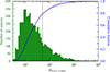 |
Fig. 6. Distribution of source counts with its cumulative distribution shown by the solid line curve. The dashed vertical line marks the threshold of 50 counts, above which we deem a spectral analysis meaningful. Only 20% of all sources are above this limit, while about half have fewer than 20 counts, as shown by the cumulative distribution (blue). |
A vital characteristic of the sample is the sources’ flux distribution. Unless stated otherwise, for consistency and as not to mix different flux determination methods and since we do not expect robust spectral fitting to be possible for the majority of sources (< 50 counts), we study the properties of the blazar population in this section using the unabsorbed source intrinsic flux in the 0.2–2.3 keV band measured assuming a fixed photon index of ΓX = 2.0 and the 21 cm NH at the source position for all sources, regardless if the counts are sufficient to determine the photon index or not. We use fluxes assuming ΓX = 2.0 since this is the expected photon index obtained when averaging across the entire population. Fluxes determined with other values for a fixed photon index (ΓX = {1.5, 1.7, 2.3}) agree to within 9.1%. The fluxes from the eRASS1 catalog (Merloni et al. 2024) are consistent within the uncertainties, with an average deviation of 18%, which might be due to the different treatment of absorption and flux determination (on average the NH from the HI4PI Collaboration 2016 is higher than the one assumed by Merloni et al. 2024). The measured fluxes span a range of almost four decades; the brightest source is 3C 273 (4FGL J1229.0+0202, FX, 0.2 − 2.3 keV = 6.2 × 10⁻¹¹ erg cm−2 s−1, with an exposure time of 111 s and 7179 counts), the faintest is WIBRaLS2 J045646.58−585411.7 (FX, 0.2 − 2.3 keV = 6.9 × 10⁻¹⁵ erg cm−2 s−1, with an exposure of 867 s and 13 counts).
About half of the sources in the BlazEr1 catalog are brighter than the flux level where completeness is reached across the western Galactic hemisphere, FX, 0.2 − 2.3 keV = 2 × 10⁻¹³ erg cm−2 s−1 (see Sect. 3.3 and Fig. 7). Fainter sources are located in parts of the sky where eROSITA has deeper exposure.
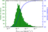 |
Fig. 7. Flux distribution in the BlazEr1 catalog. The majority of sources have fluxes below the survey completeness limit on the western Galactic hemisphere, the vertical line marks this limit. The cumulative distribution is shown in blue. |
Reliable redshifts, z, are available for 3627 catalog objects (Fig. 8). Including the S25 photometric redshifts increases the number of available values to 4795. The majority of blazars and blazar candidates are found at z < 2. The sample contains 155 sources with z ≥ 2.5, including objects up to z ∼ 6, such as the high-redshift blazar candidate BROS J1322.1−1323 (z = 4.71; Belladitta et al. 2025; Ighina et al. 2025). Among these z ≥ 2.5 sources, we report the first X-ray detection of the blazar 5BZQ J1007+1356, which was identified as a γ-ray emitter by Kreter et al. (2020) during an a posteriori search for transient γ-ray signals from high-z blazars. Out of the 87 blazars on the western Galactic hemisphere studied by Kreter et al. (2020), eROSITA detects 61 sources. Consistent with previous results (Ajello et al. 2012, 2014, 2020), the observed distribution of redshifts indicates that BLLs tend to be at low z, while FSRQs peak toward z ∼ 1.0. BCUs can be found at all redshifts. About 13% of the BLLs with measured redshifts are found at z > 0.7, which could be potentially misclassified if the infrared band is not covered (D’Elia et al. 2015). If two out of five high redshift BLLs would be misclassified, the resulting effect would have a similar impact as the contamination by changing look blazars (D’Elia et al. 2015). Therefore, given the size of the sample the overall results will not be significantly altered by not considering this in detail.
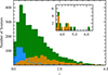 |
Fig. 8. Redshift distribution of BlazEr1 sources. The colors represent different subtypes. All BlazEr1 entries are shown in green (3627 sources), BLLs in blue, and FSRQs in orange. The inset shows the distribution for sources with z > 3.5. |
Several remarkable eROSITA-detected blazars located in the early Universe are not part of BlazEr1. eRASSU J020916−562650 is one of the most distant blazars known (z = 5.6; Wolf et al. 2024; Ighina et al. 2024), but was not detected in eRASS1, only in subsequent surveys in eRASS2, eRASS3, and eRASS4 (the name of the source deviates from the name used by Wolf et al. 2024). The z = 6.19 quasar CFHQS J142952+544717, which was detected in the first eROSITA survey (Medvedev et al. 2020), is located on the eastern Galactic hemisphere. Recent observations with Chandra and NuSTAR revealed rapid variability, identifying it as a likely blazar (Marcotulli et al. 2025). Similarly, the blazars TXS 1508+572 (z = 4.3) and GB6 1428+4217 (z = 4.7), which have shown remarkably luminous γ-ray flaring events in recent years (Gokus et al. 2024a, 2025), are also located on the eastern Galactic hemisphere.
To assess the quality of the photometric redshifts by S25 we compared them to the reliable literature (spectroscopic and photometric from, for instance, the BZCAT or 4LAC catalogs) redshifts where both parameters are available. For almost 67% of the sources the difference in redshift is > 10%. We therefore limit our population study involving distance-dependent properties (such as e.g., luminosity) to objects with reliable literature redshifts and omit the photometric redshifts of S25.
5.2. Luminosity distributions of eROSITA detected blazars
We derived rest-frame luminosities for the 0.2–2.3 keV band, LX, 0.2 − 2.3 keV8. Not surprisingly, the luminosity of the detected blazars increases with redshift, and the catalog is also biased toward higher luminosities due to the flux limit while sampling a larger volume. This bias becomes evident when comparing with other missions (see Fig. 9). The NuSTAR sample of Middei et al. (2022) tends to contain sources with higher luminosities and fluxes, covering similar values as eROSITA. Additionally, with the NuSTAR sample it can be seen that blazars are highly variable. Due to the lower sensitivity of the Swift-BAT sample (Marcotulli et al. 2022), luminosities from that sample are biased toward high luminosities, as only high-flux sources are part of this sample. The comparison with these hard X-ray samples indicates that eROSITA samples intermediate luminosities between the shallow all-sky hard X-ray samples and deeper surveys, and also extends to higher redshifts (see above).
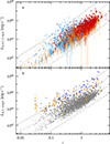 |
Fig. 9. X-ray luminosity as a function of redshift. The different dashed lines display luminosities of sources with ΓX = 2.0 for increasing z and a fixed X-ray flux: from top (dashed line) to bottom (dash-double dot line), we display FX, 0.2 − 2.3 keV from 10−11 erg cm−2 s−1 down to 10−14 erg cm−2 s−1 in steps of 10. We show the main band eROSITA luminosity in panel a, following the color scheme introduced in Fig. 3; and the 2–10 keV X-ray luminosity in panel b. In gray the BlazEr1 sample is shown. Orange points are based on NuSTAR data (Middei et al. 2022), blue points on Swift-BAT (Marcotulli et al. 2022), using the redshifts from BZCAT and 3HSP for the NuSTAR and the redshifts from Marcotulli et al. (2022) and adopting their best fit models. |
The median luminosity for all objects is LX, 0.2 − 2.3 keV ∼ 7.3 × 1044 erg s−1. Confirmed blazars show slightly higher luminosities, due to a tail toward lower luminosities apparent in the luminosity distributions (Fig. 10). On average FSRQs are more luminous by almost an order of magnitude compared to BLLs and BCUs, which have similar values. The median values for all source subgroups are given in Table 3. Since redshifts are more difficult to determine for BLLs, luminosities are available for more FSRQs than BLLs. The luminosities inferred with eROSITA are consistent with previous studies (e.g., Donato et al. 2001; Fan et al. 2012). Overall, luminosities determined for blazar candidates agree with those of confirmed blazars and no stark difference is found between γ-detected and nondetected sources. Kolmogorov-Smirnov tests indicate that most distributions differ significantly at the 95% confidence level, all combinations result in a p-value below 0.05, with the exception of the BCU and BLL distributions, which likely have the same underlying distribution (95%, p-value of 0.09). This result is consistent with previous results which hinted that most BCUs are BLLs (Kang et al. 2019; Peña-Herazo et al. 2020; Chiaro et al. 2021).
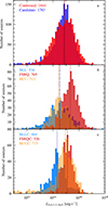 |
Fig. 10. Luminosity distribution for all sources with reliable redshifts. The panels show distributions for different subgroups of the eROSITA blazars and eROSITA blazar candidates, with vertical lines indicating the median luminosity for each subgroup (see Table 3). |
Characterization of the distribution of luminosities in BlazEr1.
The low-energy peak frequencies of the LSPs (as identified in the 4LAC) increase with decreasing luminosity. For HSPs and ISPs no significant trend is observed. This observation is consistent with the origin of the X-rays within the SED coming from different processes. The result would also be consistent with the blazar sequence, however, since the input catalog is neither complete nor statistically well defined, and since the blazar sequence might also be due to selection effects, no further conclusion can be drawn from this matching behavior.
5.3. Hardness ratios
In Fig. 11, we show the distribution of hardness ratios (see Sect. 3.4 for the definition) based on the source counts of the BlazEr1 objects. The hardness ratio diagrams highlight the difference in spectral properties among the blazar classes, revealing softer spectra for BLLs (blue) in comparison to FSRQs (red). The obtained hardness ratios have values expected if sources have absorbed power law spectra. Sources in Fig. 11 cluster toward the left of the diagrams and the tracks, therefore most objects are consistent with lower NH, as expected for the blazar population.
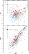 |
Fig. 11. Scatter plot of hardness ratios between energy bands 1 (0.2–0.7 keV), 2 (0.7–1.2 keV), and 3 (1.2–5.0 keV). Sources with ≥50 counts are shown in the color scheme of Fig. 3, fainter sources in gray. These sources show a higher dispersion and larger uncertainties. Dotted lines show, from top to bottom, expected hardness ratios for photon indices ΓX = 1.0, ΓX = 2.0, and ΓX = 3.0. The absorption increases along the tracks toward the top-right corner. The majority of source hardnesses are consistent with power law spectra in the expected range of spectral shapes due to the large uncertainties. The black data point in the top-left corners displays the median uncertainties of all, including the low count sources. |
5.4. Photon indices
For the 1273 blazars with ≥50 counts, more detailed information about the spectral shape is available from our spectral fits (Sect. 3.4), since for these sources constraints on the photon index can be derived9. Figure 12 shows probability distributions of the photon indices of all of these sources as well as for the various subclasses, taking into account the (sometimes large) uncertainties of the spectral fits. The distributions are approximately Gaussian; Table 4 lists the results from fitting Gaussian functions to the distributions. In order to see how similar the distributions are, we performed KS-tests on all the possible combinations, requiring a 95% confidence level. In some cases subsamples from the BlazEr1 catalog are likely to have the same underlying distribution and we list the p-values for those. All not listed combinations have different underlying distributions (p < 0.05).
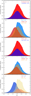 |
Fig. 12. Probability distribution of photon indices for different types of eROSITA observed blazars and blazar candidates. The distribution takes into account the uncertainties of individual measurements of the photon index. |
Fitting results for the distributions of photon indices.
The distribution of X-ray photon indices of the whole spectroscopic sample (≥50 counts) peaks at around ΓX = 2.0. This is observed for the candidates as well, indicating that a sufficient fraction of these candidates have X-ray spectra similar to blazars. A clear separation is seen between FSRQs and BLLs. Consistent with the blazar sequence (Fossati et al. 1998), FSRQs with a higher luminosity peak at lower energies due to more efficient cooling (Ghisellini et al. 1998; see Fig. 12b), resulting in harder X-ray spectra with a higher chance of the emission not being part of the low energy SED peak compared to BLLs. BCUs are overall similar to all confirmed blazars (p = 0.707), confirming their blazar nature. In Fig. 12c, we compare confirmed blazars detected in γ rays to those not detected in γ rays, noting that the distributions are quite similar. We find no difference between sources detected in the 4FGL and the overall (including those from the 4FGL catalog and those not detected in γ rays) distribution of confirmed blazars (p = 0.429) or BCUs (p = 0.138). Confirmed blazars with no γ-ray detection have similar photon indices as the overall candidate distributions (p = 0.648), those of the BLLC ( = 0.280) and BCUC (p = 0.589) classes and the BCUs (p = 0.076). The distributions of the 4FGL and non-4FGL confirmed blazars do not originate from the same underlying distribution (p < 0.001). This is also observed for the BLLs (p = 0.093) and BCUs (p = 0.972) subclasses, however, we find no difference between the γ-ray detected and the nondetected FSRQs (p = 0.008). Although the X-ray photon indices of γ-ray detected and non-γ-ray detected sources have very similar values, consistent with previous studies (e.g., Yuan & Fan 2014), the comparison of the distribution indicates different distributions, with the exception of FSRQs. A possible reason is Compton dominance and the general decoupling of X-rays and γ rays due to the different physical mechanisms. Figure 12d compares the power law slopes of different candidate populations. Although FSRQCs exhibit slightly harder spectra, the distributions of FSRQCs, BLLCs (which is similar to the confirmed distribution p = 0.705 and to BCUs p = 0.701), and BCUCs are more similar than for the confirmed objects. The BCUC distribution is similar to the other candidate subclasses (p = 0.066 for BLLCs, and 0.064 for FSRQCs). Potentially this is due to an uncertain source classification. All candidates are similar to the BLLCs (p = 0.198), and BCUCs (p = 0.893).
Figure 12e shows the photon index by SED type. LSP blazars tend to have indices below ΓX ≲ 2.0, indicating a rising X-ray spectrum, HSPs have photon indices ΓX ≳ 2.0, therefore the X-rays are part of the synchrotron peak. ISPs peak around ΓX ∼ 2.0. We emphasize again that all distributions have a large overlap with each other, indicating again that Γ alone is not a good measure of source type. As expected, FSRQs and LSPs have the same underlying photon index distribution (p = 0.272), whereas the HSPs and BLLs share similar values (p = 0.569), which is also the case for the ISPs (p = 0.680), which also exhibit a similar distribution as the HSPs (p = 0.841).
It is interesting to compare our average X-ray photon indices for the different blazar types with those derived previously. Table 4 lists a few literature values. Our results are consistent with the previous studies, despite these samples being significantly smaller. Comparing our values to the larger sample by Giommi et al. (2019) we notice that their distributions peak at different positions (Giommi et al. 2019; their Fig. 10); eROSITA spectra are slightly softer. We see an overall trend that FSRQs and BLLs show different spectral slopes, which is also observed in the literature (e.g., Giommi et al. 2019).
In our study, we also observe the split between FSRQs and BLLs in the distribution of Γ with flux (Fig. 13a). BLLs tend to have higher indices as well as higher fluxes, while FSRQs tend to show a harder index but extending toward lower fluxes. In the entire sample, we detect no correlation between flux and photon indices for the entire sample or any sub sample with the exception of BLLs showing a very weak but statistically significant anticorrelation10 (see Table B.1 for correlations coefficients). Figure 13b shows Γ as a function of luminosity. These parameters seem to be anti-correlated, as sources with harder spectra have higher luminosities, a trend already described by Kadler (2005). The anticorrelation is strongest for the FSRQs; all other sub samples have less statistically significant anticorrelations and some are not statistically significant at all. This observation is consistent with the blazar sequence, where FSRQs tend to have higher luminosities and harder indices, as the X-rays are more likely to originate from inverse Compton emission. BLLs tend to display lower luminosities and softer indices, which has already been described in the literature (e.g., Fan et al. 2012). Despite the higher X-ray luminosity of FSRQs, the highest observed fluxes (> 5 × 10⁻¹² erg cm−2 s−1) are almost exclusively from BLLs due to their prevalence at lower redshifts. Additionally, the hard spectral index of FSRQs makes it easier to detect low-flux FSRQs, while BLLs with very soft spectra and low fluxes are likely underrepresented due to the detection limits. This indicates a bias in our sample toward high-flux BLLs. For BLLs no correlation exists between the photon index and the redshift of the source, while for FSRQs we find increasingly hard spectra and high luminosities with increasing redshift. A similar observation is made for the FSRQCs. These results resemble those of Giommi et al. (2019), and are due to a selection effect.
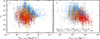 |
Fig. 13. Photon index as a function of a flux and b luminosity, following the color scheme introduced in Fig. 3 (BLL(C)s: blue, FSRQ(C)s: red, BCU(C)s: orange). |
5.5. The flux-dependent source population of eROSITA blazars
We generated log N-log S distributions using fluxes and the sensitivity, giving us the sky area, A, covered at a given limiting flux, FX (see Sect. 3.3),
 (6)
(6)
where areas sensitive to a certain flux level were obtained from the absorbed sensitivity limits of our simulation by correcting for the absorption used (NH = 1 × 1021 cm−1). To avoid contamination by Galactic point sources and those in neighboring galaxies, we excluded regions at Galactic latitudes |b|≤15° and circular regions of radius  and
and  around the Large and Small Magellanic Clouds, respectively (Fig. 4, blue line). Also, due to the large uncertainties, we also excluded all sources fainter than FX, 0.2 − 2.3 keV ∼ 6 × 10⁻¹⁴ erg cm−2 s−1, such that 4785 objects were finally included for the log N-log S calculation, including 1804 blazars (519 BLLs, 682 FSRQs, and 575 BCUs) and 2981 blazar candidates.
The log N-log S distributions are shown in Fig. 14. The faded color and dashed lines show the distributions without using the correction obtained from the simulation. These uncorrected distributions stress how important it is to take the eROSITA survey sensitivity into account. The log N-log S distribution shown here is not binned but cumulative, therefore giving uncertainties is not straightforward. The uncertainties displayed are the square root of the variance of the source number count calculated using Eq. (4) of Cappelluti et al. (2009). There is a slight deviation, or “dip”, in the distribution at fluxes around FX, 0.2 − 2.3 keV ≃ 1 × 10⁻¹¹ erg cm−2 s−1. Tests with different selection criteria, such as restricting the sources to the common footprint of the BLAZE catalog input catalogs, did not remove this feature. Based on the simulation presented in Sect. 3.3, however, we were able to exclude eROSITA’s sensitivity as the cause of this feature, as it is not present in the simulated data, which uses the as-flown eROSITA attitude. Computing log N-log S distributions for various ecliptic latitude bins for the eRASS1 catalog resulted in noisier distributions in this particular flux range, which is characterized by a small number of objects. The deviation from a smooth function became more pronounced, and we therefore concluded that this feature is most likely due to small number statistics, possibly in combination with source inhomogeneities in the sky, as also documented by Merloni et al. (2024, Sect. 5.5).
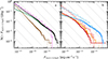 |
Fig. 14. log N-log S distributions for sources within the extragalactic sky. Panel a: comparison of the total sample of eROSITA observed blazars and blazar candidates (black) with the distribution by Giommi & Padovani, (2015, purple). Green and brown show the log N-log S for both classes separately (green: eROSITA observed blazars, brown: observed candidates). Panel b: comparison of the predictions of Giommi & Padovani (2015) for BLLs (light blue) and FSRQs (light red) with eROSITA measurements for BLLs, FSRQs, and BCUs, using the color code of Fig. 3). |
In order to compare our results to the only available predictions for the X-ray band for the log N-log S of blazars (Giommi & Padovani 2015), we converted all fluxes to the 0.3–3.5 keV band, assuming an unabsorbed power law with Γx = 2.0, since the fluxes used throughout the paper and those from the simulation have already been corrected for absorption. Our log N-log S distributions agree quite well with theoretical expectations and agree in terms of the slope. Giommi & Padovani (2015) did not assume the blazar sequence but the blazar-simplified view, which provides a reasonable explanation for the observed log N-log S distribution. However, no definitive statement about whether the blazar sequence or the blazar-simplified view is true can be made, as the overall results are consistent with both scenarios. A detailed investigation is beyond the scope of this paper. Assuming that the blazar candidates are indeed predominantly blazars, the incompleteness of the BlazEr1 catalog at high fluxes is low with respect to the prediction by Giommi et al. (2019). At the highest fluxes the prediction is lower than the observed log N-log S distribution. This discrepancy is caused by the 20 brightest blazars, which are predominantly BLLs. After cross-checking the fluxes with the unpublished eRASS2 data, we can rule out flaring as the cause of this feature. Fluxes this high are not covered by Giommi & Padovani (2015). Since the number of sources in this flux regime is negligible the discrepancy at high fluxes is due to small number statistics and thus not relevant to the overall result.
We find that confirmed blazars dominate the source numbers in the high-flux regime, with a similar trend as in the combined log N-log S distribution, with incompleteness inducing a deviation from the prediction at fluxes below 2 × 10⁻¹³ erg cm−2 s−1. At low fluxes, the blazar candidates dominate. Likely most or all blazars with high fluxes have already been identified, unlike those at low fluxes, which are therefore included in the candidate catalogs used to build the BLAZE catalog. We can also compare the distributions of the subtypes of confirmed blazars and find that incompleteness effects are seen at lower fluxes, with respect to the predictions by Giommi & Padovani (2015). At high fluxes the BLLs agree quite well with their prediction. For FSRQs the log N-log S is found below the theoretical curve but the slopes are consistent. For the BCUs, the log N-log S distribution for most part lies above that of FSRQs. All these sources either belong to the BLL or FSRQ type but have not been identified yet, explaining parts of the observed incompleteness (the majority of BCUs are thought be BLLs; Kang et al. 2019; Peña-Herazo et al. 2020; Chiaro et al. 2021). Giommi & Padovani (2015) also predict a population inversion between BLLs and FSRQs at a flux of FX, 0.3 − 3.5 keV ≃ 1 × 10⁻¹³ erg cm−2 s−1, resulting from the different slopes, which is related to the evolution and distribution of the source classes in the Universe. Such an inversion is seen in the data as well, although at a slightly higher flux, albeit this discrepancy could be due to the incompleteness of our data and other causes can not be ruled out as well.
An earlier comparison by Turriziani et al. (2019) of data with the Giommi & Padovani (2015) predictions shows a similar shape in log N-log S, although due to incompleteness the log N-log S distribution of confirmed blazars lies below the prediction and reaches down to fainter fluxes as presented here. Candidates included by Turriziani et al. (2019) resulted in upper limits for the distributions above the log N-log S expectation, therefore indicating that the candidates included might be contaminated by other sources. This observation is not reproduced here, due to a low level of contamination, however, since Turriziani et al. (2019) derived upper limits at low fluxes, both results could still be consistent. Given the lower flux limit of Turriziani et al. (2019) and the fact that their sample is a flux limited one, whereas the BlazEr1 catalog sample is not, a detailed comparison is not straightforward. Therefore, no disagreement with the previous results can be found.
The slopes of log N-log S distributions have implications for the cosmological evolution of blazars (e.g., Maccacaro et al. 1987; Langejahn et al. 2020; Marcotulli et al. 2022). A slope of α = 1.5 implies no cosmological evolution, that is, the sources are uniformly distributed in the Universe. Less steep slopes indicate a negative cosmological evolution, where sources are more common in the local Universe and their density declines with increasing redshift. On the other hand steeper slopes correspond to a positive evolution and more or brighter sources at higher redshifts than in the local Universe. We determined slopes for all the observed distributions, taking flux uncertainties into account by using a Monte-Carlo approach and assuming that fluxes follow a normal distribution. We fitted a power law in the form of
 (7)
(7)
to the 0.2–2.3 keV log N-log S distribution11, limiting ourselves to fluxes FX, 0.2 − 2.3 keV ≥ 3 × 10⁻¹³ erg cm−2 s−1 to avoid incompleteness effects. The resulting parameters are listed in Table 5 and the best-fit functions are shown in Fig. A.3. The normalization for the best fit to the BLLs is too low compared to the observed distribution, an effect due to the flattening caused by incompleteness, beaming effects (Marcotulli et al. 2022), and the low number of sources at high fluxes; however, the slope matches well. All measured slopes are below or close to 1.5, therefore we find almost all subtypes and the overall eROSITA observed blazars to be consistent with negative cosmological evolution. For the blazar candidates the slope is close to no evolution at all or a slightly positive one. As the log N-log S distribution possibly shows breaks, we also considered a broken power law as a fit function for the entire sample using the same fit approach. One possible break is found at FX, break, 0.2 − 2.3 keV = (2.11 ± 0.26)×10−12 erg cm−2 s−1, although a second less significant solution exits with the break at a slightly smaller flux value. The position of the break could coincide with the flux region in which FSRQs start to be detected but is also close to the previously described dip and could therefore be a survey effect not related to blazars at all. Specific modeling of the log N-log S and an analysis of the cosmological evolution of blazars, which would require a very detailed study of the luminosity function and modeling it with different evolutionary scenarios, is beyond the scope of this paper.
log N-log S distributions fit results.
Older studies were based on comparably few sources, reducing the significance of some conclusions. Previous work has indicated a positive evolution for FSRQs (Wolter & Celotti 2001; Toda et al. 2017; Turriziani et al. 2019; Marcotulli et al. 2022). For BLLs, different trends have been observed, depending on the underlying source sample. Slightly positive to no evolution has been found for BLLs of the LSP type (Stickel et al. 1991). HSPs have been found to be consistent with negative evolution (Rector et al. 2000). In hard X-ray selected samples, FSRQs are found to evolve positively, whereas BLLs show no or negative evolution (Ajello et al. 2009; Toda et al. 2017; Marcotulli et al. 2022). For γ-ray selected samples BLLs also follow a positive evolution, with the exception of HSPs, which show a negative evolution (Ajello et al. 2014). However, the slope reported by Langejahn et al. (2020) for a radio selected Swift-BAT sample is close to the one reported in our work, indicating a negative evolution as well. The hard X-ray log N-log S by Langejahn et al. (2020) shows a significant difference in slope compared to their radio input sample. Langejahn et al. attributed this to different evolution of the X-ray and radio emission, with the former having a peak at z ∼ 1.5. Our results using eROSITA support this conclusion, as the soft X-rays seen by eROSITA exhibit similar properties as the hard X-ray sources studied by Langejahn et al. (2020), although the evolution found by them is different than in other studies (e.g., Toda et al. 2017; Marcotulli et al. 2022).
The number of blazars eROSITA was supposed to detect has been predicted in the literature assuming that soft and hard X-ray log N-log S-distributions are similar. Toda et al. (2017) predicted eROSITA to observe 13 900 FSRQs and 1900 BLLs on the entire sky within four years. We did indeed detect slightly more FSRQs than BLLs, since at low fluxes, more FSRQs are observed by roughly an order of magnitude. The prediction would require the vast majority of unclassified sources to be FSRQs, which would be inconsistent with the expectation that BCUs are more likely BLLs. Considering that the actual eROSITA survey is less sensitive than assumed, the numbers at least somewhat agree as a rough order-of magnitude estimate.
Marcotulli et al. (2022) predicted that in its first year eROSITA would have observed 230 023 FSRQs with fluxes FX, 0.2 − 2.0 keV ≥ 1 × 10⁻¹⁴ erg cm−2 s−1 across the entire sky and across a wide range of redshifts. The BlazEr1 catalog does not contain even 1% of this predicted amount of sources. Considering the best fit to the log N-log S distribution for the FSRQ sample, ∼2.17 deg−2 are expected to be observed, corresponding to 89654 FSRQs over the entire sky, which only corresponds to 39% of the predicted number. The discrepancy is in part caused by Marcotulli et al. (2022) assuming a different, deeper, limiting flux level. Additionally, the assumed slopes of the log N-log S distribution are different and both estimates assume that the slope at higher fluxes is the same at low fluxes, which might not be the case.
5.6. Past X-ray observations and properties of eROSITA detected blazars
In this section, we compare our eROSITA results with those from other missions, for sources which are detected in both. Since earlier work estimated fluxes assuming power law slopes with ΓX = 1.7 or similar (OUSXB: ΓX = 1.8), when comparing results in this subsection, we consistently use eROSITA-fluxes obtained assuming ΓX = 1.7, even in cases where we (or authors of other works) were able to constrain the spectral shape.
ROSAT, as the precursor of eROSITA, sets the benchmark for all-sky surveys at soft X-ray energies. Due to the different spatial accuracies we matched the eROSITA detected sources with a quite large radius ≤40″, hence this comparison is more prone to potential mismatches. In total we obtained 1496 matches between eROSITA and ROSAT and in total 1865 ROSAT sources coinciding with BLAZE catalog objects on the western Galactic hemisphere within 40″. Of the ROSAT BLAZE catalog matches, 108 are included in the unverified BlazEr1 catalog, while 261 sources detected by ROSAT are not detected by eROSITA. Therefore, eROSITA is able to recover 84% of the blazars and blazar candidates detected by ROSAT. Since eROSITA is sensitive over the entire sky down to a similar flux limit as ROSAT (FX, 0.1 − 2.4 keV = 10−13 erg cm−2 s−1, Boller et al. 2016), the sources not included in the BlazEr1 catalogs are probably missing due to variability. The fluxes measured by ROSAT agree with the eROSITA fluxes within the eROSITA uncertainties in only 9.5% of the matches. Variability is present and the majority of sources are within the same order of magnitude. There are 543 objects with ROSAT fluxes higher by more than an order of magnitude, whereas for the reverse, only five cases are observed. This subsample of high-flux ROSAT matches does not grow or shrink in number with different angular separations between the source positions of the two missions. A similar trend with respect to XMM-Newton is reported by Boller et al. (2016, their Fig. 25), probably caused by spurious ROSAT detections combined with systematic differences between the instruments, such as energy coverage and sensitivity. The ROSAT photon indices are not well constrained, have large uncertainties and do not correlate with the eROSITA ones. This is likely due to the different signal-to-noise levels and the restricted energy coverage of ROSAT.
For sources both in the eROSITA and the Swift-XRT catalog (Evans et al. 2020), we confidently detected 1249 of the 1700 matches within the eRASS1 footprint between Evans et al. (2020) and the BLAZE catalog, assuming a maximum separation of 8″. 451 sources are not part of the BlazEr1 catalog and eROSITA picks up 73% of the Swift-XRT detected blazars and blazar candidates. The fluxes are broadly consistent, although only 25% of the matches agree with each other within the uncertainties. However, many sources tend to have higher fluxes in Swift-XRT than in eROSITA: for 57% of the sources the flux in eROSITA is at least 30% less than in Swift-XRT. This higher flux is caused partly by variability, but also due to the fact that the approach of Evans et al. (2020) uses all available data for a given source position, such that these flux values represent the combination of different flux states of a source, with a bias toward brighter states. Many Swift-XRT observations are triggered following flaring states, explaining a bias toward brighter states. Sensitivity differences between the instruments might also play a role. The photon indices mostly agree with each other, with a slight trend toward somewhat softer photon indices measured with eROSITA (ΔΓX ∼ 0.05).
A similar picture presents itself when comparing our catalog to the OUSXB (Giommi et al. 2019). Similar to Evans et al. (2020), this catalog uses all Swift-XRT observations, however, the catalog offers data for each individual observation. In terms of total numbers, OUSXB DR3 contains 1223 BLAZE catalog sources in the western Galactic hemisphere (Giommi et al. 2019; 2508 BLAZE catalog sources are listed for the entire sky), of which 1039 are confidently detected and an additional 85 objects are part of the unverified catalog. This means that only 99 sources go completely undetected by eROSITA.
The BlazEr1 catalog lists 2106 confirmed blazars, therefore it is the largest collection of X-ray detected blazars on the western Galactic sky by a factor of 1.7. Taking the blazar candidates into account, the BlazEr1 catalog encompasses the largest sample of X-ray detected blazars and blazar-candidates to this day. In Fig. 15 we compare the mean flux value of Giommi et al. (2019) with our flux. Generally, the fluxes are consistent with each other within the eROSITA uncertainties and the maximum and minimum value provided by Giommi et al. (2019). In ∼48% of sources, we observe flux variations due to source variability. However, due to a slightly different photon index being used and due to the observational biases by Swift-XRT in terms of including all data and therefore also including flares, for more than 50% of the sources the fluxes do not agree. The same has already been observed when comparing to the catalog by Evans et al. (2020). Generally, the photon indices are consistent with each other with ∼68% of the values agreeing within the uncertainties of eROSITA and the maximum and minimum values given in the OUSXB (Fig. 16). Overall, there seems to be a slight trend of deriving softer photon indices using eROSITA compared to Swift-XRT (mean ΔΓX ∼ 0.08, with 17% of the sources having a diverging photon index of at least 1σ deviation). This may be explained by the harder-when-brighter trend in connection with the bias of Swift-XRT observations toward flaring states. Overall, the results derived from eROSITA data are consistent with previous studies.
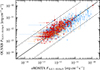 |
Fig. 15. Swift-XRT flux reported by Giommi et al. (2019) as a function of eROSITA flux, following the color scheme introduced in Fig. 3. The mean values of all measurements for a source listed in Giommi et al. (2019) are shown. The uncertainties of the Swift-XRT fluxes represent the minimum and maximum values provided by Giommi et al. (2019). The solid line represents the unity line, while the dashed ones indicate a factor 10 difference between the measurements. |
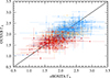 |
Fig. 16. Mean photon indices derived by Swift-XRT using Giommi et al. (2019) and eROSITA, following the color scheme introduced in Fig. 3. The uncertainties of the Swift-XRT photon indices represent the minimum and maximum values provided by Giommi et al. (2019). The solid line represents unity. Differences are observed, indicating that blazars are variable in their spectral properties. |
For the hard X-rays we compare our soft X-ray fluxes with the hard X-ray fluxes obtained by Swift-BAT (Lien et al. 2025) and NuSTAR (Middei et al. 2022). Very few sources are identified in the Swift-BAT data. The Swift-BAT fluxes are all in a similar range and we test how these hard X-ray fluxes correlate with the eROSITA flux. Swift-BAT picks up more FSRQs and BCUs, and they tend to have slightly higher fluxes in Swift-BAT compared to BLLs, for which all correlations are insignificant. For the softer NuSTAR band higher fluxes in eROSITA correspond to higher fluxes in NuSTAR. In the harder band, the trends are quite similar but appear with weaker significance. The photon indices of NuSTAR and Swift-BAT are similar to those observed by eROSITA, establishing a linear correlation between indices in the soft and hard X-ray band.
Finally, we stress that many of the BlazEr1 sources were never observed with other X-ray missions. It contains 5611 and 5546 sources that have never been observed by XMM-Newton and Chandra, respectively. Other missions show similar high numbers of unobserved sources (ASCA: 5730, NuSTAR: 5772, Suzaku: 5822, Swift-XRT: 4069 and ROSAT: 4331). We find that 2966 BlazEr1 sources (51% of the BlazEr1 catalog) have no prior X-ray observations with any of the listed missions. Considering only confirmed blazars, 31% of these were never observed with any pointed X-ray instrument. The sample of previously unobserved blazars is dominated by FSRQs and BCUs. Since BLLs are more easily detected due to their higher X-ray fluxes, they might be targeted more often, such that previous missions will have more exposure time at positions associated with BLLs. Due to the large amount of new X-ray data, eROSITA enables us to study a more complete picture of the blazar population.
5.7. Multiwavelength properties of the BlazEr1 sources
In this section, we combine eROSITA data with multiwavelength data available for BlazEr1 sources (see Sect. 4). We discuss the γ-ray, radio, infrared, and optical properties and how the properties in the different wavelength regimes are connected with the X-rays.
5.7.1. The γ-ray emission of BlazEr1 sources
In Figure 17 we compare the X-ray and γ-ray fluxes of the BlazEr1 sources. We fitted a linear function in log-space (log10(Fγ, 0.2 − 100 GeV) = m × log10(FX, 0.2 − 2.3 keV) + t) to the distributions, and calculated correlation coefficients. For FSRQs, a dense cloud indicating a direct correlation of X-ray and γ-ray fluxes can be seen, although the correlation is weak. The distributions of BLLs and BCUs are more spread out and most likely not correlated. Since almost all FSRQs belong to the class of LSPs, a correlation between X-ray and γ-ray emission is somewhat expected as the emission is expected to be produced by the same emission mechanism. For BLLs and BCUs, which consist of a mix of LSPs, ISPs, and HSPs, a correlation is less straightforward, but from FX, 0.2 − 2.3 keV ∼ 2 × 10⁻¹² erg cm−2 s−1 on, sources with higher X-ray fluxes also seem to have higher γ-ray fluxes. Additionally, we observe that in general, sources with a γ-ray detection have higher X-ray fluxes than the non-γ-ray detected ones, which has also been previously reported by Paliya et al. (2017).
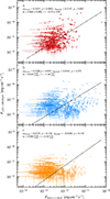 |
Fig. 17. Fermi-LAT fluxes (4FGL-DR4; Abdollahi et al. 2022) compared with eROSITA fluxes. The three panels show the different subtypes, following the color scheme introduced in Fig. 3 (a: FSRQs, b: BLLs, c: BCUs). The Fermi-LAT uncertainties are scaled to match the confidence limit of the eROSITA data. |
In Fig. 18 we compare the Fermi-LAT photon indices to the eROSITA photon indices. There is a clear separation between BLLs and FSRQs. On average, the X-ray index of BLLs is softer than the γ-ray index, while for FSRQs the opposite is observed. This is partly due to the different SED types these classes are mainly associated with. However, roughly 4% of the BLLs are occupying the same region as the FSRQs, which are mostly classified as LSPs. The BCUs are distributed among the different groups. Previous studies (e.g., Comastri et al. 1997; Fan et al. 2012; Yuan & Fan 2014) have found that the X-ray and γ-ray photon indices of the entire blazar population are anti-correlated. This trend is seen for the overall sample as well (see Fig. 18), however, not as strongly and there also seem to be differences for the subgroups. For the entire sample we found a best fit with a linear fit function (Γγ = m × ΓX + t) with fit values between the ones reported by Fan et al. (2012) and Yuan & Fan (2014). We emphasize that the correlation is relatively weak but significant. The subgroups show no correlation, with the exception of a very weak anticorrelation for BCUs.
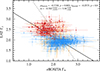 |
Fig. 18. Fermi-LAT photon index (4FGL-DR4; Abdollahi et al. 2022) compared with the eROSITA photon index, following the color scheme introduced in Fig. 3 (BLLs: blue, FSRQs: red, BCUs: orange). In solid, the linear best fit is shown, additionally the correlation between the two parameters found by Yuan & Fan (2014; dashed) and Fan et al. (2012; dotted) are displayed. The uncertainties of Γγ are extrapolated to the 90% confidence interval. |
We note that the data compared here have not been taken simultaneously, and we compare X-ray fluxes taken at a specific time (during eRASS1) with γ-ray fluxes from the 4FGL-DR4 averaged over 14 years. Hence, variability can make the interpretation difficult.
5.7.2. Radio emission of BlazEr1 sources
In Fig. 19, we show the flux densities obtained from TANAMI, MOJAVE, and RFC as a function of eROSITA flux. Of the 52 TANAMI matches, the majority belongs to the FSRQ class, as this program targets γ-ray detected sources up to a limiting radio flux density, as well as highly variable jetted non-blazar AGNs. Flux densities in TANAMI mostly increase as a function of eROSITA flux and we find a strong correlation for FSRQs. Almost twice as many objects are matched with MOJAVE (97); the overall trends are similar to TANAMI and a correlation with the eROSITA flux is found as well. The RFC contains radio flux densities for 2620 BlazEr1 sources. Again a similar trend of the flux densities being correlated as in TANAMI and MOJAVE is observed for FSRQs. Based on the RFC data, we find that for BLLs flux densities in the radio are similar, regardless of the X-ray flux and no strong correlation is found. This behavior is also observed for the BLLs in TANAMI and MOJAVE, although the number of individual objects is very low compared to the RFC and the correlations found are not statistically significant. Again, the different physical origin of the emission is likely driving the diverging behavior between the FSRQs and BLLs. Of the radio flux limited sample of HBL sources by Giommi et al. (2020), five out of twelve sources on the western Galactic hemisphere are included in the BlazEr1 catalog.
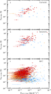 |
Fig. 19. Correlation of radio flux densities and eROSITA fluxes, following the color scheme introduced in Fig. 3, using a data from the TANAMI program, b data from MOJAVE, and c X-band flux densities from the RFC catalog. |
5.7.3. Infrared and optical properties of eROSITA-detected blazars
Infrared colors are commonly used to characterize different types of AGNs (e.g., Salvato et al. 2018; their Fig. 9). In the infrared color-color diagram (Fig. 20), blazars occupy a distinct region due to the nonthermal emission of the jet, which enables good distinction from thermal emitters (e.g., Massaro et al. 2011; D’Abrusco et al. 2012; Massaro et al. 2012a,b; Massaro & D’Abrusco 2016; Salvato et al. 2018; de Menezes et al. 2019). Most of the sources in BlazEr1 are contained within the locus initially described by Massaro et al. (2011) to be associated with jet emission in the WISE color-color space displayed in Fig. 20. Using all WISE colors, the region containing γ-ray emitting blazars has been well characterized, establishing the WISE γ-ray strip (D’Abrusco et al. 2012; Massaro et al. 2012a). The initial location by Massaro et al. (2011), which has not been formally characterized, is considered a projection of the higher dimensional WISE γ-ray strip (Massaro & D’Abrusco 2016). We therefore, find our blazars to be consistent with the initial location by Massaro et al. (2011) and the WISE γ-ray strip (Massaro & D’Abrusco 2016). This region in the color-color diagram also covers the region usually occupied by QSOs and Seyfert galaxies, and extends toward spiral and elliptical galaxies. Objects located far from this region are mostly blazar candidates of some kind, although sources associated with confirmed blazars are found in other parts of the color-color diagram as well. A high number of BCUCs are found in the regions associated with starburst, spiral, and elliptical galaxies, as well as stars. The infrared colors also separate the BLLs and FSRQs as they are found in different regions. BLLs tend to have bluer colors than the FSRQs. BCUs are found in similar loci as BLLs and FSRQs.
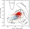 |
Fig. 20. WISE color-color diagram, following the color scheme introduced in Fig. 3. Regions populated by different types of AGNs, as well as other objects, are shown. Compare our results to Salvato et al. (2018; Fig. 9), for a color-color diagrams of the 2RXS and XMMSL2 samples. |
We were able to combine the infrared data with optical and X-ray information. In Fig. 21 we show four different photometric spaces, which can be used to distinguish between Galactic and extragalactic sources and see if objects exhibit similar properties as other AGNs (Salvato et al. 2022). The (g − r)–(z − W1) color-color diagram is shown in Fig. 21a. Most BlazEr1 sources are above the dotted line and thus consistent with being extragalactic. There are many candidates, as well as a small number of confirmed sources below this line, hinting at a low level of contamination (see Sect. 3.2).
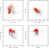 |
Fig. 21. Different photometric spaces combining optical, infrared and X-ray data, similar to Salvato et al. (2022; Fig. 18) for point sources detected in eFEDS, using the color scheme introduced in Fig. 3. Solid gray lines show positions usually occupied by quasars, whereas the gray dotted lines corresponded to Seyfert 2 galaxies. The dashed black lines in the top panels distinguish between Galactic and extragalactic sources. |
A sequence parallel to the separation line can be identified as well, mainly consisting of candidates, BCUs, and BZGs, which is typically the location of quiescent galaxies. Salvato et al. (2022) show a similar trend with redshift, where sources at low redshifts are more red. This trend is also observed in our sample, since FSRQs are typically found at higher redshifts and are also located at bluer colors. In Fig. 21b we show the W1 magnitude as a function of X-ray flux. This information can be used to check the extragalactic content, although the separation line shown becomes a less robust indicator as the X-ray survey increases in size (Salvato et al. 2022). While most sources are consistent with an extragalactic origin, the objects below this line are BCUCs, again indicating that the catalog is subject to some degree of contamination. The optical-infrared color-color diagram (Fig. 21c), which can be used to distinguish stars from AGNs, does not exhibit a sequence of most likely Galactic sources as seen in Salvato et al. (2022), maybe due to the incompleteness of Gaia. The tail at high values of g − W1 corresponding to inactive galaxies is less pronounced and mainly occupied by candidates (BCUCs and BLLCs). The WISE color-magnitude diagram (Fig. 21d) can be used to identify stars (typically W1 − W2 ∼ 0.0, marked with a dashed line) and quasars. Most objects are quasar-like.
The BlazEr1 sources are located where we expect to observe AGNs and only very few are located elsewhere and are inconsistent with an extragalactic nature. Overall, sources are similar to QSOs (solid gray line) and extend toward the loci of Seyferts (dotted gray line), where we also find a high number of candidates. The infrared and optical data show that the catalog might have some degree of contamination by other source types, although a detailed source-by-source analysis would be required to see if sources with data typical for non-blazars are in fact contaminants.
5.7.4. Broadband spectral indices of the eROSITA blazars
As detailed in Sect. 4.5, we computed broadband spectral indices, αij, for different bands from the radio to the γ rays to relate the X-rays to other bands. For a given SED, the observed spectral index will depend on the peak frequencies and the luminosities of the SED peaks. A value α > 1.0 indicates a negative slope in νFν space, meaning the SED decreases toward higher energies. We display the broadband spectral indices as calculated from various bands against each other in Fig. 22. For objects that are also in the 4LAC, in Fig. A.4, we show the indices as a function of Compton dominance, the ratio of the peak fluxes, and low- and high-energy SED peak frequencies (Ajello et al. 2020, 2022). Additionally, we calculated correlation coefficients for different parameter combinations to assess the correlations between parameters for the entire sample and the BLL and FSRQ sub samples. The results are listed in Tables B.2 and B.3 and mean values obtained for the broadband spectral indices are shown in Table B.4.
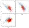 |
Fig. 22. Broadband spectral indices αXΓ, αIRX, and αRX against each other, following the color scheme introduced in Fig. 3. Due to the similar values obtained for αOX and αIRX, the former is not shown here. |
FSRQs mostly show values of αXΓ ∼ 1.0, that is they show no significant increase or decrease from the X-rays toward the γ rays, which is expected, since X-rays are more likely to cover the rise of the high-energy peak and the γ rays cover the fall of the same peak. The values of αXΓ do not correlate significantly with the peak positions but there is a significant weak anticorrelation with Compton dominance (see Fig. A.4i and Table B.2). As indicated by the values of αOX, a decreasing slope from the optical toward the X-rays is observed for a majority of FSRQs, and no correlation with the SED parameters is found. Similar results are found for αIRX, however, the slopes are slightly steeper and the dispersion is smaller (see Table B.4), perhaps due to FSRQs displaying a big blue bump which adds flux in the infrared–UV range (Krauß et al. 2016). A very weak correlation between the infrared X-ray spectral index αIRX and the low-energy peak position is present. Only extreme cases of FSRQs with low-energy peaks in the radio range are found to decrease from the radio toward the X-rays, however, the vast majority of sources show an increase. We find a very weak anticorrelation between αRX and the low-energy peak position.
For BLLs both rising and falling indices from the X-rays to the γ rays are observed, but the mean value indicates a flat index. Sources with decreasing slopes have their high-energy peak at energies below GeV γ rays, where Fermi-LAT is sensitive, and show low Compton dominance. Larger values of αXΓ are linked to higher peak frequencies, as this parameter is moderately and weakly correlated with the low- and high-energy peak frequencies, respectively, and a lower Compton dominance, with a weak anticorrelation being present. The values of αOX indicate that for BLLs, on average a decreasing slope from the optical toward the X-rays is observed. However, some sources exhibit an increase that corresponds to extreme HSPs. In general, a higher spread of values is seen than for FSRQs. In most cases the low-energy peak occurs at energies lower than the X-ray band and an increase in the value of αOX corresponds to a lower peak frequency for the low-energy peak, but this anticorrelation is very weak. An anticorrelation with the peak frequency of the high-energy peak is observed, however, we find no correlation with Compton dominance.
We observe a very similar picture for the infrared range. BLLs are found at more extreme decreasing and increasing slopes toward the X-ray band than the FSRQs as indicated by the larger spread. We observe only a weak anticorrelation with the position of the low-energy peak and a moderate one with the high-energy peak. BLLs show a stronger increase from the radio band toward the X-rays than FSRQs and a higher dispersion. We see a moderate anticorrelation with the SED peak positions. Since in many BLLs the radio and X-ray emission are thought to originate from the same process, a trend between peak positions and α-values is expected, as lower values in α correspond to peak positions at higher energies. Candidates and confirmed blazars show similar behavior without significant offsets. The BCUs are consistent with being blazars of either type.
For αXΓ we find a significantly strong or moderate anticorrelation with all other indices, however, the correlation is different for FSRQs and BLLs, as for the BLLs the anticorrelations are stronger. There is a weaker anticorrelation between αXΓ for FSRQs and the other ranges, consistent with the X-rays covering the dip of the low-energy peak or the rise of the high-energy peak in the SED. For BLLs the anticorrelation is stronger, and for lower αXΓ values, these BLLs have higher Compton dominance and lower peak frequencies (LSP). The αOX and αIRX indices have higher values compared to αXΓ, which is the opposite of αRX. For the BLLs a strong correlation is found with the αRX and the infrared and optical. For the FSRQs we find no or only very weak correlations. This is expected, as in many BLLs these bands share the same emission process origin, showing strong correlations, whereas for FSRQs the X-rays originate from the high-energy peak but the other bands are related to the low-energy peak. The correlation between αOX and αIRX is a strong or moderate one, with αOX having slightly higher values. The weaker correlation for FSRQs is probably due to the big blue bump (Krauß et al. 2016; and references therein).
The values derived for αOX are similar to those found in the literature (see, e.g., Giommi et al. 1999; Turriziani et al. 2007). Broadband spectral indices for the γ rays and X-rays have also been provided for example by Comastri et al. (1997) using EGRET, however, their values (FSRQs: αXΓ = 0.58 ± 0.12, BLLs: αXΓ = 0.83 ± 0.18) are lower than ours, probably due to the lower energy band covered in the γ rays.
No significant strong or moderate correlations can be found between the photon indices and values of α, however, the subclasses show different trends. We found only weak correlations for BLLs with αIRX and αOX and a weak anticorrelation with αXΓ. Anticorrelations from some samples with αRX are observed. Moderate correlations between the α-value and redshift are observed. The αXΓ, decreases with redshift, while αRX increases.
Since values of α correlate with the SED peaks and Compton dominance, selection cuts could be applied to identify sources with different SED types or certain peak positions. In particular, αIRX, αOX, and αRX could be useful to classify the sources into HSP (αRX < 0.69, αIRX < 1.12) and LSP (αRX > 0.87, 1.5 > αIRX > 1.0) categories. For ISP it is not possible to find boundaries that separate them from the other SED types well. For the HSP constraints, 69% of classifications agree with the SED definition when compared to the 4LAC catalog; for LSPs more than 96% are recovered. The BlazEr1 catalog contains 127 blazars within the HSP constraints outlined, these could potentially be TeV blazars (see Metzger et al. 2025), and 812 sources within the proposed LSP criteria. Sources with values close to αIRX ∼ 1.2, αOX ∼ 1.2, and αRX ∼ 1.0 could be MeV blazars, and are interesting targets for future MeV missions (e.g., COSI; Tomsick et al. 2019, 2024).
5.8. Why some sources go undetected
We went on to consider objects that have not been detected by eROSITA, or only at low significance. In Table 6, we list the number of detected sources from each input catalog, also distinguishing among the different classes, with respect to the western Galactic hemisphere, and considering the quality cuts to the BLAZE catalog. Overall, only ∼14% of all BLAZE catalog sources are part of the BlazEr1 catalog, however, ∼69% of the gold sample (confirmed blazars in the BLAZE catalog) is detected. Due to eROSITA’s all-sky survey strategy and higher sensitivity we miss less than one third of the confirm blazar population, a significant improvement to Swift-XRT (43%, Giommi et al. 2019).
Completeness of the BlazEr1 catalog.
The BZCAT, 4FGL, and 3HSP catalogs exhibit the highest detection fraction among all input catalogs, as they contain the most extensive list of confirmed blazars. The fact that the 4FGL has such a high detection rate implies that γ rays are a good indicator for a subsequent X-ray detection, which is connected to the fact that the γ-ray detected sources have brighter X-ray fluxes. The HighZ objects are less likely to be detected, probably due to their faintness given their high redshifts. The candidates also have a lower detection rate, which is due to contamination and these sources generally being fainter. The Milliquas catalog, which mainly adds candidates to the BLAZE catalog, has a high-detection rate as well, due to also containing many confirmed blazars. Other candidate catalogs exhibit detection rates between 8% and 58%. The BROS catalog has the lowest detection rate, despite having the highest number of input sources. A large contributing factor is the increased level of contamination compared to other catalogs.
Among the confirmed blazars, BLLs and FSRQs have slightly higher detection rates than BCUs, of which only more than half are detected. This could mean that BCUs also contain more contaminating objects, and that their X-ray fluxes are too low to be detected. The different candidate classes have lower detection rates. eROSITA is more likely to detect FSRQCs than other candidate classes.
As a next step we used the eROSITA sensitivity (see Sect. 3.3) to obtain the flux and luminosity upper limits for the undetected blazars and blazar candidates. The majority of nondetected sources have upper limits below the flux at which the all-sky survey is complete (Fig. 4). The upper limits agree with those of Tubín-Arenas et al. (2024). Since Tubín-Arenas et al. (2024) also considered the counts actually observed by eROSITA, their upper limits are sometimes higher than ours.
As a next step, we calculate luminosity upper limits for sources with known redshifts (Fig. 23). The exposure times, fluxes and luminosity limits are all listed in the BLAZE catalog. At low redshifts, BCUs in particular are abundant. We also observe FSRQs at higher redshifts than BLLs as previously seen in Sect. 5.2. The dashed-dotted line in Fig. 23, which corresponds to a flux of FX, 0.2 − 2.3 keV = 1 × 10⁻¹⁴ erg cm−2 s−1, indicates that the lower luminosity population is missed due to the sensitivity limit of eROSITA.
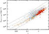 |
Fig. 23. X-ray luminosity as a function of redshift, following the color scheme introduced in Fig. 3. BlazEr1 sources are shown in gray. The colored symbols are sources with low DET_LIKE, quality issues or a high angular separation. The added lines are the same as in Fig. 9. The upper limits have been taken from the BLAZE catalog. |
Similarly to Fig. 17, we compare the X-ray upper limits to γ-ray fluxes in Fig. 24. The majority of nondetections correspond to BCUs, found at lower γ-ray fluxes than detected sources. Of the undetected blazars with a counterpart in the 4LAC catalog, the majority are LSPs (265 objects), ISPs and HSPs are less prominent (76 and 29, respectively). LSPs are expected to exhibit harder spectra, which hints at a potential bias toward softer and more high peaked objects, which are easier to detect. It is likely that all these sources were missed in eRASS1 due to being faint. These results indicate that subsequent all-sky survey releases by eROSITA will have higher detection rates than the BlazEr1 catalog, as the faintness of the sources represents one of the main limitations for our catalog.
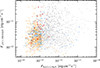 |
Fig. 24. Fermi-LAT flux as a function of eROSITA flux, following the color scheme introduced in Fig. 3. The gray points are BlazEr1 sources, whereas sources without a significant detection are shown in color. Arrows indicate the upper limits. |
6. Summary and future work
We present the Blazars in eRASS1 (BlazEr1) catalog of blazars and blazar candidates detected by eROSITA on the western Galactic hemisphere. This catalog is available online through Vizier and at the eROSITA DR1 webpage12. The catalog was derived by matching a master list of blazars and blazar candidate sources from the literature (the BLAZE catalog, released together with this paper) to the eROSITA eRASS1 catalog (Merloni et al. 2024). We used the classes given in the input catalogs the BLAZE catalog has been constructed from, since the fraction of misclassifications, including the changing-look objects, is expected to be only roughly 5%. Considering the size of the BLAZE and BlazEr1 catalogs, this has a negligible impact on our conclusions. After applying quality cuts, a set of 5865 eROSITA observed blazars and blazar candidates were detected. The eROSITA sources removed during processing steps have been released in a separate catalog. The BlazEr1 catalog has been augmented with X-ray spectral and multiwavelength information (see Appendix D). To date, this catalog is the most complete compilation of confirmed X-ray detected blazars on the western Galactic hemisphere and, to our knowledge, the largest catalog of X-ray detected blazars and blazar candidates. Overall, the BlazEr1 catalog is expected to contain at most 633 contaminating sources (Sect. 3.2).
The main scientific results obtained from an analysis of the catalog include the distribution of photon indices for the spectroscopic sample (Sect. 5.4), which clearly show that the different blazar subtypes exhibit distinct spectral properties, enabling tentative determinations of the subtype based on the photon index. The relations between the spectral properties and fluxes and luminosities are consistent with expectations from the blazar sequence (Sect. 5.4). We find that eROSITA is more sensitive toward low-flux FSRQs than low-flux BLLs, probably due to the very soft spectra displayed by the latter. Most of the brightest blazars detected are BLLs, while the fluxes of γ-ray detected sources are higher than those of the non γ-ray detected ones.
The slopes of the log N-log S distributions constructed from the catalog imply a negative cosmological evolution, both for the entire sample and for different subsamples, meaning the objects are more common in the Local Universe; however, for the blazar candidates, the value could indicate a slight positive evolution (Sect. 5.5). The observed distributions agree well with theoretical predictions (Giommi & Padovani 2015). We find evidence for a population inversion between BLLs and FSRQs at lower fluxes.
The spectral properties, fluxes, and luminosities of the BCUs are similar to low flux BLLs, consistent with other publications (Sect. 5.2; Kang et al. 2019; Peña-Herazo et al. 2020; Chiaro et al. 2021). The multiwavelength data help to separate blazars into their respective classes using color-color diagrams and highlights the importance of the eROSITA data for building a comprehensive blazar catalog and studying their properties, as well as for future SED modeling (Sect. 5.7).
The BlazEr1 catalog can serve as a benchmark for overall blazar properties and single-object properties since it provides the first X-ray observation for many blazars. For instance, the eROSITA data will be crucial to constrain the SEDs of a large number of objects, including samples such as those from TANAMI, MOJAVE, or 4FGL. Earlier applications of the eRASS1 catalog included the identification of X-ray counterparts for an ultra-high-energy neutrino event (Adriani et al. 2025) and the identification of TeV blazar candidates for follow-up observations (Metzger et al. 2025; see also Marchesi et al. 2025).
Additionally, the eROSITA surveys allow for a detailed variability study on timescales of hours-days for the brightest and on a half-year time line for all other sources. The BlazEr1 catalog provides the framework for these studies. Examples include work on X-ray blazar flares, as demonstrated, for instance, for PKS 0735+178 (Hämmerich et al. 2021b; Sahakyan et al. 2022) or a γ-ray flare of TXS 0646−176 (Hämmerich et al. 2021a).
A subsequent data release of 2.2 years of data (eRASS:5), will allows us to provide an updated, deeper version of the catalog. The cumulative eROSITA data will also deepen the catalog, making the eRASS:5 version, which will contain 2.2 years of data, the deepest X-ray blazar catalog ever constructed.
Data availability
The BLAZE and BlazEr1 catalogs are available at the CDS via https://cdsarc.cds.unistra.fr/viz-bin/cat/J/A+A/709/A37 and the eROSITA DR1 webpage https://erosita.mpe.mpg.de/dr1/AllSkySurveyData_dr1/Catalogues_dr1/
Acknowledgments
S.H. is partly supported by the German Science Foundation (DFG grant numbers WI 1860/14-1 and 434448349). Mi.K. acknowledges support from DLR grant FKZ 50 OR 2307. Ma.K. and F.R. acknowledge funding by the Deutsche Forschungsgemeinschaft (DFG, German Research Foundation, grant 434448349). A.G.M. acknowledges support from Narodowe Centrum Nauki (NCN) grant 2018/31/G/ST9/03224. Ma.K. E.R. and J.W. gratefully acknowledge funding by the Deutsche Forschungsgemeinschaft (DFG, German Research Foundation), within the research unit 5195 “Relativistic Jets in Active Galaxies” under project number 443220636. This work is part of the M2FINDERS (ERC grant No. 101018682) and ASTROGEODESY (ERC grant No. 101076060) projects, funded by the European Research Council under the EU Horizon 2020 Research and Innovation Programme. This work is based on data from eROSITA, the soft X-ray instrument aboard SRG, a joint Russian-German science mission supported by the Russian Space Agency (Roskosmos), in the interests of the Russian Academy of Sciences represented by its Space Research Institute (IKI), and the Deutsches Zentrum für Luft- und Raumfahrt (DLR). The SRG spacecraft was built by Lavochkin Association (NPOL) and its subcontractors, and was operated by NPOL with support from the Max Planck Institute for Extraterrestrial Physics (MPE). The development and construction of the eROSITA X-ray instrument was led by MPE, with contributions from the Dr. Karl Remeis Observatory Bamberg and ECAP (FAU Erlangen-Nürnberg), the University of Hamburg Observatory, the Leibniz Institute for Astrophysics Potsdam (AIP), and the Institute for Astronomy and Astrophysics of the University of Tübingen, with the support of DLR and the Max Planck Society. The Argelander Institute for Astronomy of the University of Bonn and the Ludwig Maximilians Universität Munich also participated in the science preparation for eROSITA. The eROSITA data shown here were processed using the eSASS/NRTA software system developed by the German eROSITA consortium. This research has made use of ISIS functions (ISISscripts) provided by ECAP/Remeis observatory and MIT (https://www.sternwarte.uni-erlangen.de/isis/). This research has made use of data, software and/or web tools obtained from the High Energy Astrophysics Science Archive Research Center (HEASARC), a service of the Astrophysics Science Division at NASA/GSFC and of the Smithsonian Astrophysical Observatory’s High Energy Astrophysics Division, and of the Vizier and HEASARC database systems for querying objects and getting information from different catalogs. We thank Tess Jaffe (GSFC) for valuable input concerning our HEASARC queries. This work has also made use of data from the European Space Agency (ESA) mission Gaia (https://www.cosmos.esa.int/gaia), processed by the Gaia Data Processing and Analysis Consortium (DPAC, https://www.cosmos.esa.int/web/gaia/dpac/consortium). Funding for the DPAC has been provided by national institutions, in particular the institutions participating in the Gaia Multilateral Agreement. The SIMBAD database, operated at CDS, Strasbourg, France, was also used to get additional information.
References
- Abdo, A. A., Ackermann, M., Ajello, M., et al. 2009, ApJ, 707, L142 [NASA ADS] [CrossRef] [Google Scholar]
- Abdo, A. A., Ackermann, M., Agudo, I., et al. 2010, ApJ, 716, 30 [NASA ADS] [CrossRef] [Google Scholar]
- Abdollahi, S., Acero, F., Ackermann, M., et al. 2020, ApJS, 247, 33 [Google Scholar]
- Abdollahi, S., Acero, F., Baldini, L., et al. 2022, ApJS, 260, 53 [NASA ADS] [CrossRef] [Google Scholar]
- Ackermann, M., Ajello, M., Atwood, W. B., et al. 2015, ApJ, 810, 14 [NASA ADS] [CrossRef] [Google Scholar]
- Adriani, O., Aiello, S., Albert, A., et al. 2025, ApJ, submitted [arXiv:2502.08484] [Google Scholar]
- Agarwal, A., Gupta, A. C., Bachev, R., et al. 2015, MNRAS, 451, 3882 [Google Scholar]
- Ahnen, M. L., Ansoldi, S., Antonelli, L. A., et al. 2018, A&A, 620, A181 [NASA ADS] [CrossRef] [EDP Sciences] [Google Scholar]
- Ajello, M., Costamante, L., Sambruna, R. M., et al. 2009, ApJ, 699, 603 [NASA ADS] [CrossRef] [Google Scholar]
- Ajello, M., Shaw, M. S., Romani, R. W., et al. 2012, ApJ, 751, 108 [NASA ADS] [CrossRef] [Google Scholar]
- Ajello, M., Romani, R. W., Gasparrini, D., et al. 2014, ApJ, 780, 73 [Google Scholar]
- Ajello, M., Angioni, R., Axelsson, M., et al. 2020, ApJ, 892, 105 [NASA ADS] [CrossRef] [Google Scholar]
- Ajello, M., Baldini, L., Ballet, J., et al. 2022, ApJS, 263, 24 [NASA ADS] [CrossRef] [Google Scholar]
- An, T., Wang, A., Liu, Y., et al. 2023, MNRAS, 519, 4047 [CrossRef] [Google Scholar]
- Antonucci, R. 1993, ARA&A, 31, 473 [Google Scholar]
- Atwood, W. B., Abdo, A. A., Ackermann, M., et al. 2009, ApJ, 697, 1071 [CrossRef] [Google Scholar]
- Belladitta, S., Moretti, A., Caccianiga, A., et al. 2019, A&A, 629, A68 [NASA ADS] [CrossRef] [EDP Sciences] [Google Scholar]
- Belladitta, S., Moretti, A., Caccianiga, A., et al. 2020, A&A, 635, L7 [EDP Sciences] [Google Scholar]
- Belladitta, S., Bañados, E., Xie, Z.-L., et al. 2025, A&A, 699, A335 [NASA ADS] [CrossRef] [EDP Sciences] [Google Scholar]
- Bellenghi, C., Padovani, P., Resconi, E., & Giommi, P. 2023, ApJ, 955, L32 [NASA ADS] [CrossRef] [Google Scholar]
- Beringer, J., Arguin, J. F., Barnett, R. M., et al. 2012, Phys. Rev. D, 86, 010001 [CrossRef] [Google Scholar]
- Blandford, R. D., & Königl, A. 1979, ApJ, 232, 34 [Google Scholar]
- Blandford, R. D., & Rees, M. J. 1978, in Pittsburgh Conference on BL Lac Objects, ed. A. M. Wolfe (University of Pittsburgh Department of Physics and Astronomy), 328 [Google Scholar]
- Blandford, R., Meier, D., & Readhead, A. 2019, ARA&A, 57, 467 [NASA ADS] [CrossRef] [Google Scholar]
- Bloom, S. D., & Marscher, A. P. 1996, ApJ, 461, 657 [NASA ADS] [CrossRef] [Google Scholar]
- Boller, Th., Freyberg, M. J., Trümper, J., et al. 2016, A&A, 588, A103 [NASA ADS] [CrossRef] [EDP Sciences] [Google Scholar]
- Böttcher, M., Reimer, A., Sweeney, K., & Prakash, A. 2013, ApJ, 768, 54 [Google Scholar]
- Brunner, H., Liu, T., Lamer, G., et al. 2022, A&A, 661, A1 [NASA ADS] [CrossRef] [EDP Sciences] [Google Scholar]
- Caccianiga, A., Moretti, A., Belladitta, S., et al. 2019, MNRAS, 484, 204 [NASA ADS] [CrossRef] [Google Scholar]
- Cappelluti, N., Brusa, M., Hasinger, G., et al. 2009, A&A, 497, 635 [NASA ADS] [CrossRef] [EDP Sciences] [Google Scholar]
- Cash, W. 1979, ApJ, 228, 939 [Google Scholar]
- Chang, Y. L., Arsioli, B., Giommi, P., Padovani, P., & Brandt, C. H. 2019, A&A, 632, A77 [NASA ADS] [CrossRef] [EDP Sciences] [Google Scholar]
- Chiaro, G., Kovacevic, M., & La Mura, G. 2021, J. High En. Astrophys., 29, 40 [Google Scholar]
- Ciaramella, A., Bongardo, C., Aller, H. D., et al. 2004, A&A, 419, 485 [NASA ADS] [CrossRef] [EDP Sciences] [Google Scholar]
- Comastri, A., Fossati, G., Ghisellini, G., & Molendi, S. 1997, ApJ, 480, 534 [Google Scholar]
- Coppejans, R., Frey, S., Cseh, D., et al. 2016, MNRAS, 463, 3260 [Google Scholar]
- D’Abrusco, R., Massaro, F., Ajello, M., et al. 2012, ApJ, 748, 68 [CrossRef] [Google Scholar]
- D’Abrusco, R., Álvarez Crespo, N., Massaro, F., et al. 2019, ApJS, 242, 4 [Google Scholar]
- D’Ammando, F., Orienti, M., Finke, J., et al. 2015, MNRAS, 446, 2456 [Google Scholar]
- Dauser, T., Falkner, S., Lorenz, M., et al. 2019, A&A, 630, A66 [NASA ADS] [CrossRef] [EDP Sciences] [Google Scholar]
- de la Calle Pérez, I., Álvarez Crespo, N., Racero, E., & Rouco, A. 2021, A&A, 655, A48 [NASA ADS] [CrossRef] [EDP Sciences] [Google Scholar]
- de Menezes, R., Peña-Herazo, H. A., Marchesini, E. J., et al. 2019, A&A, 630, A55 [NASA ADS] [CrossRef] [EDP Sciences] [Google Scholar]
- de Vaucouleurs, G., de Vaucouleurs, A., & Corwin, H. G. 1976, Second Reference Catalogue of Bright Galaxies (University of Texas Press: Austin) [Google Scholar]
- D’Elia, V., Padovani, P., Giommi, P., & Turriziani, S. 2015, MNRAS, 449, 3517 [Google Scholar]
- Dermer, C. D., & Schlickeiser, R. 1993, ApJ, 416, 458 [Google Scholar]
- Dey, A., Schlegel, D. J., Lang, D., et al. 2019, AJ, 157, 168 [Google Scholar]
- Donato, D., Ghisellini, G., Tagliaferri, G., & Fossati, G. 2001, A&A, 375, 739 [NASA ADS] [CrossRef] [EDP Sciences] [Google Scholar]
- Donato, D., Sambruna, R. M., & Gliozzi, M. 2005, A&A, 433, 1163 [NASA ADS] [CrossRef] [EDP Sciences] [Google Scholar]
- Evans, P. A., Page, K. L., Osborne, J. P., et al. 2020, ApJS, 247, 54 [Google Scholar]
- Fan, J. H., Yang, J. H., Yuan, Y. H., Wang, J., & Gao, Y. 2012, ApJ, 761, 125 [Google Scholar]
- Finke, J. D. 2016, ApJ, 830, 94 [Google Scholar]
- Fitzpatrick, E. L. 1999, PASP, 111, 63 [Google Scholar]
- Flesch, E. W. 2023, OJAp, 6, 49 [NASA ADS] [Google Scholar]
- Fossati, G., Maraschi, L., Celotti, A., Comastri, A., & Ghisellini, G. 1998, MNRAS, 299, 433 [Google Scholar]
- Gatuzz, E., Wilms, J., Hämmerich, S., & Arcodia, R. 2024, A&A, 683, A213 [NASA ADS] [CrossRef] [EDP Sciences] [Google Scholar]
- Gehrels, N. 1986, ApJ, 303, 336 [Google Scholar]
- Ghisellini, G. 2013, EPJ Web Conf., 61, 05001 [NASA ADS] [CrossRef] [EDP Sciences] [Google Scholar]
- Ghisellini, G., & Madau, P. 1996, MNRAS, 280, 67 [CrossRef] [Google Scholar]
- Ghisellini, G., Celotti, A., Fossati, G., Maraschi, L., & Comastri, A. 1998, MNRAS, 301, 451 [NASA ADS] [CrossRef] [Google Scholar]
- Ghisellini, G., Sbarrato, T., Tagliaferri, G., et al. 2014, MNRAS, 440, L111 [CrossRef] [Google Scholar]
- Ghisellini, G., Haardt, F., Ciardi, B., et al. 2015a, MNRAS, 452, 3457 [Google Scholar]
- Ghisellini, G., Tagliaferri, G., Sbarrato, T., & Gehrels, N. 2015b, MNRAS, 450, L34 [NASA ADS] [CrossRef] [Google Scholar]
- Ginzburg, V. L., & Syrovatskii, S. I. 1965, ARA&A, 3, 297 [Google Scholar]
- Giommi, P., & Padovani, P. 2015, MNRAS, 450, 2404 [Google Scholar]
- Giommi, P., Menna, M. T., & Padovani, P. 1999, MNRAS, 310, 465 [NASA ADS] [CrossRef] [Google Scholar]
- Giommi, P., Padovani, P., & Perlman, E. 2000, MNRAS, 317, 743 [NASA ADS] [CrossRef] [Google Scholar]
- Giommi, P., Padovani, P., Polenta, G., et al. 2012, MNRAS, 420, 2899 [NASA ADS] [CrossRef] [Google Scholar]
- Giommi, P., Brandt, C. H., Barres de Almeida, U., et al. 2019, A&A, 631, A116 [NASA ADS] [CrossRef] [EDP Sciences] [Google Scholar]
- Giommi, P., Chang, Y. L., Turriziani, S., et al. 2020, A&A, 642, A141 [NASA ADS] [CrossRef] [EDP Sciences] [Google Scholar]
- Gokus, A., Paliya, V. S., Wagner, S. M., et al. 2021, A&A, 649, A77 [NASA ADS] [CrossRef] [EDP Sciences] [Google Scholar]
- Gokus, A., Böttcher, M., Errando, M., et al. 2024a, ApJ, 974, 38 [Google Scholar]
- Gokus, A., Wilms, J., Kadler, M., et al. 2024b, MNRAS, 529, 1450 [Google Scholar]
- Gokus, A., Errando, M., Agudo, I., et al. 2025, ApJ, 990, 206 [Google Scholar]
- Gordon, Y. A., Rudnick, L., Andernach, H., et al. 2023, ApJS, 267, 37 [NASA ADS] [CrossRef] [Google Scholar]
- Hämmerich, S., Gokus, A., Kreykenbohm, I., Rau, A., & Wilms, J. 2021a, ATel 14991 [Google Scholar]
- Hämmerich, S., Zainab, A., Gokus, A., et al. 2021b, ATel 15108 [Google Scholar]
- Harrison, F. A., Craig, W. W., Christensen, F. E., et al. 2013, ApJ, 770, 103 [Google Scholar]
- Healey, S. E., Romani, R. W., Cotter, G., et al. 2008, ApJS, 175, 97 [Google Scholar]
- HI4PI Collaboration. 2016, A&A, 594, A116 [NASA ADS] [CrossRef] [EDP Sciences] [Google Scholar]
- Hinton, J. A., & Hofmann, W. 2009, ARA&A, 47, 523 [NASA ADS] [CrossRef] [Google Scholar]
- Homan, D. C., Ojha, R., Wardle, J. F. C., et al. 2002, ApJ, 568, 99 [NASA ADS] [CrossRef] [Google Scholar]
- Homan, D. C., Cohen, M. H., Hovatta, T., et al. 2021, ApJ, 923, 67 [NASA ADS] [CrossRef] [Google Scholar]
- Houck, J. C., & Denicola, L. A. 2000, ASP Conf. Ser., 216, 591 [Google Scholar]
- Ighina, L., Caccianiga, A., Moretti, A., et al. 2019, MNRAS, 489, 2732 [NASA ADS] [CrossRef] [Google Scholar]
- Ighina, L., Caccianiga, A., Moretti, A., et al. 2024, A&A, 692, A241 [NASA ADS] [CrossRef] [EDP Sciences] [Google Scholar]
- Ighina, L., Caccianiga, A., Moretti, A., et al. 2025, A&A, 698, A158 [NASA ADS] [CrossRef] [EDP Sciences] [Google Scholar]
- Itoh, R., Utsumi, Y., Inoue, Y., et al. 2020, ApJ, 901, 3 [NASA ADS] [CrossRef] [Google Scholar]
- Jones, T. W., O’Dell, S. L., & Stein, W. A. 1974, ApJ, 188, 353 [NASA ADS] [CrossRef] [Google Scholar]
- Kaastra, J. S. 2017, A&A, 605, A51 [NASA ADS] [CrossRef] [EDP Sciences] [Google Scholar]
- Kaastra, J. S., & Bleeker, J. A. M. 2016, A&A, 587, A151 [NASA ADS] [CrossRef] [EDP Sciences] [Google Scholar]
- Kadler, M. 2005, Ph.D. Thesis, Rheinische Friedrich Wilhelms-Universität Bonn, Bonn, Germany [Google Scholar]
- Kang, S.-J., Li, E., Ou, W., et al. 2019, ApJ, 887, 134 [Google Scholar]
- Kang, S.-J., Lyu, B., Wu, Q., Zheng, Y.-G., & Fan, J. 2024, ApJ, 962, 122 [NASA ADS] [CrossRef] [Google Scholar]
- Kapanadze, B. Z. 2013, AJ, 145, 31 [NASA ADS] [CrossRef] [Google Scholar]
- Keenan, M., Meyer, E. T., Georganopoulos, M., Reddy, K., & French, O. J. 2021, MNRAS, 505, 4726 [NASA ADS] [CrossRef] [Google Scholar]
- Khamitov, I. M., Bikmaev, I. F., Gilfanov, M. R., et al. 2022, Astron. Lett., 48, 828 [Google Scholar]
- Khorunzhev, G. A., Meshcheryakov, A. V., Medvedev, P. S., et al. 2021, Astron. Lett., 47, 123 [NASA ADS] [CrossRef] [Google Scholar]
- Kluge, M., Comparat, J., Liu, A., et al. 2024, A&A, 688, A210 [NASA ADS] [CrossRef] [EDP Sciences] [Google Scholar]
- Komossa, S., Voges, W., Xu, D., et al. 2006, AJ, 132, 531 [NASA ADS] [CrossRef] [Google Scholar]
- König, O., Wilms, J., Arcodia, R., et al. 2022, Nature, 605, 248 [CrossRef] [Google Scholar]
- Kovlakas, K., Zezas, A., Andrews, J. J., et al. 2021, MNRAS, 506, 1896 [NASA ADS] [CrossRef] [Google Scholar]
- Krauß, F., Wilms, J., Kadler, M., et al. 2016, A&A, 591, A130 [NASA ADS] [CrossRef] [EDP Sciences] [Google Scholar]
- Krauß, F., Kreter, M., Müller, C., et al. 2018, A&A, 610, L8 [NASA ADS] [CrossRef] [EDP Sciences] [Google Scholar]
- Kreter, M., Gokus, A., Krauss, F., et al. 2020, ApJ, 903, 128 [NASA ADS] [CrossRef] [Google Scholar]
- Kudenko, M., & Troitsky, S. 2024, A&A, 686, A178 [NASA ADS] [CrossRef] [EDP Sciences] [Google Scholar]
- Lacy, M., Baum, S. A., Chandler, C. J., et al. 2020, PASP, 132, 035001 [Google Scholar]
- Langejahn, M., Kadler, M., Wilms, J., et al. 2020, A&A, 637, A55 [NASA ADS] [CrossRef] [EDP Sciences] [Google Scholar]
- Lien, A. Y., Krimm, H. A., Markwardt, C. B., et al. 2025, ApJ, 989, 161 [Google Scholar]
- Liodakis, I., & Petropoulou, M. 2020, ApJ, 893, L20 [Google Scholar]
- Lister, M. L., Homan, D. C., Kellermann, K. I., et al. 2021, ApJ, 923, 30 [NASA ADS] [CrossRef] [Google Scholar]
- Maccacaro, T., Romaine, S., & Schmitt, H. M. M. 1987, IAU Symp., 124, 597 [Google Scholar]
- Madejski, G. G., & Sikora, M. 2016, ARA&A, 54, 725 [NASA ADS] [CrossRef] [Google Scholar]
- Mannheim, K. 1993, A&A, 269, 67 [NASA ADS] [Google Scholar]
- Mannheim, K., & Biermann, P. L. 1992, A&A, 253, L21 [NASA ADS] [Google Scholar]
- Maraschi, L., Ghisellini, G., & Celotti, A. 1992, ApJ, 397, L5 [CrossRef] [Google Scholar]
- Marchesi, S., Iuliano, A., Prandini, E., et al. 2025, A&A, 693, A142 [NASA ADS] [CrossRef] [EDP Sciences] [Google Scholar]
- Marcotulli, L., Ajello, M., Urry, C. M., et al. 2022, ApJ, 940, 77 [NASA ADS] [CrossRef] [Google Scholar]
- Marcotulli, L., Connor, T., Bañados, E., et al. 2025, ApJ, 979, L6 [Google Scholar]
- Marscher, A. P., & Gear, W. K. 1985, ApJ, 298, 114 [Google Scholar]
- Martí, J., Sánchez-Ayaso, E., Luque-Escamilla, P. L., et al. 2020, MNRAS, 492, 4291 [Google Scholar]
- Massaro, F., & D’Abrusco, R. 2016, ApJ, 827, 67 [NASA ADS] [CrossRef] [Google Scholar]
- Massaro, E., Tramacere, A., Perri, M., Giommi, P., & Tosti, G. 2006, A&A, 448, 861 [NASA ADS] [CrossRef] [EDP Sciences] [Google Scholar]
- Massaro, F., D’Abrusco, R., Ajello, M., Grindlay, J. E., & Smith, H. A. 2011, ApJ, 740, L48 [NASA ADS] [CrossRef] [Google Scholar]
- Massaro, F., D’Abrusco, R., Tosti, G., et al. 2012a, ApJ, 750, 138 [NASA ADS] [CrossRef] [Google Scholar]
- Massaro, F., D’Abrusco, R., Tosti, G., et al. 2012b, ApJ, 752, 61 [NASA ADS] [CrossRef] [Google Scholar]
- Massaro, E., Maselli, A., Leto, C., et al. 2015, Ap&SS, 357, 75 [Google Scholar]
- Mattox, J. R., Bertsch, D. L., Chiang, J., et al. 1993, ApJ, 410, 609 [Google Scholar]
- Medvedev, P., Sazonov, S., Gilfanov, M., et al. 2020, MNRAS, 497, 1842 [Google Scholar]
- Mereghetti, S., Tiengo, A., Esposito, P., et al. 2009, Science, 325, 1222 [NASA ADS] [CrossRef] [Google Scholar]
- Merloni, A., Predehl, P., Becker, W., et al. 2012, ArXiv e-prints [arXiv:1209.3114] [Google Scholar]
- Merloni, A., Lamer, G., Liu, T., et al. 2024, A&A, 682, A34 [NASA ADS] [CrossRef] [EDP Sciences] [Google Scholar]
- Metzger, C., Gokus, A., & Errando, M. 2025, ApJ, 992, 184 [Google Scholar]
- Middei, R., Giommi, P., Perri, M., et al. 2022, MNRAS, 514, 3179 [NASA ADS] [CrossRef] [Google Scholar]
- Mücke, A., & Protheroe, R. J. 2001, Astropart. Phys., 15, 121 [Google Scholar]
- Mücke, A., Protheroe, R. J., Engel, R., Rachen, J. P., & Stanev, T. 2003, Astropart. Phys., 18, 593 [Google Scholar]
- Müller, C., Krauß, F., Dauser, T., et al. 2015, A&A, 574, A117 [NASA ADS] [CrossRef] [EDP Sciences] [Google Scholar]
- Müller, C., Kadler, M., Ojha, R., et al. 2018, A&A, 610, A1 [NASA ADS] [CrossRef] [EDP Sciences] [Google Scholar]
- O’Dowd, M., Urry, C. M., & Scarpa, R. 2002, ApJ, 580, 96 [Google Scholar]
- Ojha, R., Kadler, M., Böck, M., et al. 2010, A&A, 519, A45 [NASA ADS] [CrossRef] [EDP Sciences] [Google Scholar]
- Padovani, P., & Giommi, P. 1996, MNRAS, 279, 526 [Google Scholar]
- Paggi, A., Bonato, M., Raiteri, C. M., et al. 2020, A&A, 641, A62 [NASA ADS] [CrossRef] [EDP Sciences] [Google Scholar]
- Paliya, V. S., & Stalin, C. S. 2016, ApJ, 820, 52 [Google Scholar]
- Paliya, V. S., Marcotulli, L., Ajello, M., et al. 2017, ApJ, 851, 33 [NASA ADS] [CrossRef] [Google Scholar]
- Paliya, V. S., Ajello, M., Rakshit, S., et al. 2018, ApJ, 853, L2 [NASA ADS] [CrossRef] [Google Scholar]
- Park, T., Kashyap, V. L., Siemiginowska, A., et al. 2006, ApJ, 652, 610 [Google Scholar]
- Peña-Herazo, H. A., Amaya-Almazán, R. A., Massaro, F., et al. 2020, A&A, 643, A103 [NASA ADS] [CrossRef] [EDP Sciences] [Google Scholar]
- Perlman, E. S., Stocke, J. T., Schachter, J. F., et al. 1996a, ApJS, 104, 251 [NASA ADS] [CrossRef] [Google Scholar]
- Perlman, E. S., Stocke, J. T., Wang, Q. D., & Morris, S. L. 1996b, ApJ, 456, 451 [Google Scholar]
- Petrov, L. Y., & Kovalev, Y. Y. 2025, ApJS, 276, 38 [NASA ADS] [CrossRef] [Google Scholar]
- Pian, E., Vacanti, G., Tagliaferri, G., et al. 1998, ApJ, 492, L17 [NASA ADS] [CrossRef] [Google Scholar]
- Pineau, F. X., Derriere, S., Motch, C., et al. 2017, A&A, 597, A89 [NASA ADS] [CrossRef] [EDP Sciences] [Google Scholar]
- Predehl, P., Andritschke, R., Arefiev, V., et al. 2021, A&A, 647, A1 [EDP Sciences] [Google Scholar]
- Puccetti, S., Capalbi, M., Giommi, P., et al. 2011, A&A, 528, A122 [NASA ADS] [CrossRef] [EDP Sciences] [Google Scholar]
- Rajput, B., Stalin, C. S., & Rakshit, S. 2020, A&A, 634, A80 [NASA ADS] [CrossRef] [EDP Sciences] [Google Scholar]
- Rakshit, S., Stalin, C. S., Chand, H., & Zhang, X.-G. 2017, ApJS, 229, 39 [Google Scholar]
- Rector, T. A., Stocke, J. T., Perlman, E. S., Morris, S. L., & Gioia, I. M. 2000, AJ, 120, 1626 [NASA ADS] [CrossRef] [Google Scholar]
- Rees, M. J. 1967, MNRAS, 137, 429 [NASA ADS] [Google Scholar]
- Rigoselli, M., De Grandis, D., Mereghetti, S., & Malacaria, C. 2023, MNRAS, 523, 3043 [Google Scholar]
- Romani, R. W., Sowards-Emmerd, D., Greenhill, L., & Michelson, P. 2004, ApJ, 610, L9 [Google Scholar]
- Ruan, J. J., Anderson, S. F., Plotkin, R. M., et al. 2014, ApJ, 797, 19 [NASA ADS] [CrossRef] [Google Scholar]
- Sahakyan, N., Giommi, P., Padovani, P., et al. 2022, MNRAS, 519, 1396 [CrossRef] [Google Scholar]
- Sahu, S., López Fortín, C. E., Valadez Polanco, I. A., & Rajpoot, S. 2021, ApJ, 914, 120 [Google Scholar]
- Salvato, M., Buchner, J., Budavári, T., et al. 2018, MNRAS, 473, 4937 [Google Scholar]
- Salvato, M., Wolf, J., Dwelly, T., et al. 2022, A&A, 661, A3 [NASA ADS] [CrossRef] [EDP Sciences] [Google Scholar]
- Salvato, M., Wolf, J., Dwelly, T., et al. 2025, A&A, 704, A344 [NASA ADS] [CrossRef] [EDP Sciences] [Google Scholar]
- Sambruna, R. M., Barr, P., Giommi, P., et al. 1994a, ApJS, 95, 371 [Google Scholar]
- Sambruna, R. M., Barr, P., Giommi, P., et al. 1994b, ApJ, 434, 468 [Google Scholar]
- Saxena, A., Salvato, M., Roster, W., et al. 2024, A&A, 690, A365 [NASA ADS] [CrossRef] [EDP Sciences] [Google Scholar]
- Sbarrato, T., Ghisellini, G., Nardini, M., et al. 2012, MNRAS, 426, L91 [Google Scholar]
- Sbarrato, T., Ghisellini, G., Nardini, M., et al. 2013, MNRAS, 433, 2182 [NASA ADS] [CrossRef] [Google Scholar]
- Sbarrato, T., Ghisellini, G., Tagliaferri, G., et al. 2015, MNRAS, 446, 2483 [NASA ADS] [CrossRef] [Google Scholar]
- Sbarrato, T., Ghisellini, G., Tagliaferri, G., et al. 2022, A&A, 663, A147 [NASA ADS] [CrossRef] [EDP Sciences] [Google Scholar]
- Sbarrato, T., Belladitta, S., Wolf, J., et al. 2026, A&A, submitted [arXiv:2603.24659] [Google Scholar]
- Schlickeiser, R. 1996, A&AS, 120, 481 [Google Scholar]
- Seppi, R., Comparat, J., Bulbul, E., et al. 2022, A&A, 665, A78 [NASA ADS] [CrossRef] [EDP Sciences] [Google Scholar]
- Shemmer, O., Brandt, W. N., Schneider, D. P., et al. 2006, ApJ, 644, 86 [NASA ADS] [CrossRef] [Google Scholar]
- Sikora, M., Begelman, M. C., & Rees, M. J. 1994, ApJ, 421, 153 [Google Scholar]
- Singh, V., & Chand, H. 2018, MNRAS, 480, 1796 [NASA ADS] [CrossRef] [Google Scholar]
- Sowards-Emmerd, D., Romani, R. W., & Michelson, P. F. 2003, ApJ, 590, 109 [Google Scholar]
- Stickel, M., Padovani, P., Urry, C. M., Fried, J. W., & Kuehr, H. 1991, ApJ, 374, 431 [Google Scholar]
- Stocke, J. T., Morris, S. L., Gioia, I. M., et al. 1991, ApJS, 76, 813 [Google Scholar]
- Sunyaev, R., Arefiev, V., Babyshkin, V., et al. 2021, A&A, 656, A132 [NASA ADS] [CrossRef] [EDP Sciences] [Google Scholar]
- Tananbaum, H., Avni, Y., Branduardi, G., et al. 1979, ApJ, 234, L9 [Google Scholar]
- Tanihata, C., Urry, C. M., Takahashi, T., et al. 2001, ApJ, 563, 569 [CrossRef] [Google Scholar]
- Toda, K., Inoue, Y., Tanaka, Y., & Fukazawa, Y. 2017, in 7 Years of MAXI: Monitoring X-ray Transients, eds. M. Serino, M. Shidatsu, W. Iwakiri, & T. Mihara (Wako, Saitama, Japan: The Institute of Physical and Chemical Research (RIKEN)), 221 [Google Scholar]
- Tomsick, J., Zoglauer, A., Sleator, C., et al. 2019, BAAS, 51, 98 [Google Scholar]
- Tomsick, J., Boggs, S., Zoglauer, A., et al. 2024, in 38th International Cosmic Ray Conference (Trieste: PoS), PoS(ICRC2023), 745 [Google Scholar]
- Truemper, J. 1982, Adv. Space Res., 2, 241 [Google Scholar]
- Truemper, J. 1993, Science, 260, 1769 [Google Scholar]
- Tubín-Arenas, D., Krumpe, M., Lamer, G., et al. 2024, A&A, 682, A35 [NASA ADS] [CrossRef] [EDP Sciences] [Google Scholar]
- Turriziani, S., Cavazzuti, E., & Giommi, P. 2007, A&A, 472, 699 [NASA ADS] [CrossRef] [EDP Sciences] [Google Scholar]
- Turriziani, S., Fraga, B., & Giommi, P. 2019, MNRAS, 489, 3307 [Google Scholar]
- Urry, C. M. 1996, ASP Conf. Ser., 110, 391 [Google Scholar]
- Urry, C. M., & Padovani, P. 1995, PASP, 107, 803 [NASA ADS] [CrossRef] [Google Scholar]
- Urry, C. M., Sambruna, R. M., Worrall, D. M., et al. 1996, ApJ, 463, 424 [Google Scholar]
- Urry, C. M., Scarpa, R., O’Dowd, M., et al. 2000, ApJ, 532, 816 [NASA ADS] [CrossRef] [Google Scholar]
- Verner, D. A., Ferland, G. J., Korista, K. T., & Yakovlev, D. G. 1996, ApJ, 465, 487 [Google Scholar]
- Véron-Cetty, M. P., & Véron, P. 2010, A&A, 518, A10 [Google Scholar]
- Voges, W., Aschenbach, B., Boller, Th., et al. 1999, A&A, 349, 389 [NASA ADS] [Google Scholar]
- Voges, W., Aschenbach, B., Boller, T., et al. 2000, IAU Circ., 7432, 3 [NASA ADS] [Google Scholar]
- Wenger, M., Ochsenbein, F., Egret, D., et al. 2000, A&AS, 143, 9 [NASA ADS] [CrossRef] [EDP Sciences] [Google Scholar]
- Wilms, J., Allen, A., & McCray, R. 2000, ApJ, 542, 914 [Google Scholar]
- Wolf, J., Salvato, M., Belladitta, S., et al. 2024, A&A, 691, A30 [NASA ADS] [CrossRef] [EDP Sciences] [Google Scholar]
- Wolter, A., & Celotti, A. 2001, A&A, 371, 527 [NASA ADS] [CrossRef] [EDP Sciences] [Google Scholar]
- Worrall, D. M., & Wilkes, B. J. 1990, ApJ, 360, 396 [Google Scholar]
- Worsley, M. A., Fabian, A. C., Turner, A. K., Celotti, A., & Iwasawa, K. 2004, MNRAS, 350, 207 [Google Scholar]
- Xie, Z.-L., Bañados, E., Belladitta, S., et al. 2024, ApJ, 964, 98 [Google Scholar]
- Yuan, Y., & Fan, J. 2014, Ap&SS, 352, 207 [Google Scholar]
- Yuan, W., Matsuoka, M., & Ueno, S. 2000, BAAS, 32, 1183 [Google Scholar]
- Yuan, W., Fabian, A. C., Celotti, A., & Jonker, P. G. 2003, MNRAS, 346, L7 [NASA ADS] [CrossRef] [Google Scholar]
Throughout the paper, we use DR3, based on 15 years of Swift-XRT data, with 2831 distinct blazars.
Catalog available at https://blaz4r.brera.inaf.it/
DET_LIKE_0 equals the negative logarithm of the probability of detected counts being caused by fluctuations of the background.
pany is the probability given by NWAY that any of the matches found is the correct counterpart.
https://heasarc.gsfc.nasa.gov/cgi-bin/W3Browse/w3browse.pl using the following distances between the source and all pointings:  for XMM-Newton,
  for Chandra,
  for ASCA,
  for NuSTAR,
  for Suzaku,
  for Swift-XRT, and 1.0° for ROSAT.
This leads to seven candidates having 4LAC parameter values as well, however, given the size of the catalog these data points can be ignored and do not influence our results in any way.
http://astrogeo.org/rfc/, covering the S (2.2–2.4 GHz), C (4.1–5.0 GHz), X (7.3–8.8 GHz), U (15.2–15.5 GHz), and K (22.0–24.2 GHz) bands.
Since we use ΓX = 2, the K-correction to transform to the rest-frame, (1 + z)ΓX − 2 = 1 (Langejahn et al. 2020).
For the spectroscopic sample we use the fluxes determined assuming ΓX = 2.0 for consistency.
For the correlation p-values we adapt the following: > 0.10: correlation does not exist, 0.10–0.05: exists but weak, 0.05–0.003: exists with moderate strength, < 0.003: exists with high significance, if numbers are orders of magnitude smaller for the high significance we just give the threshold value. If based on the p-value a correlation does not exist or the coefficient is within the range −0.1 and +0.1, we do not list the correlation coefficient and p-value. Values are listed in Table B.1.
The conversion between flux bands does not impact the slope.
Appendix A: Supplemental figures
In this appendix, we extend the discussion of the main part of this paper with further diagnostic information. Figures A.1 and A.2 display the distributions of the normalized angular separation with respect to S25. In Fig. A.3 the fits to the log N-log S distributions are shown and Fig. A.4 summarizes the relation between SED parameters and broadband spectral indices.
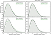 |
Fig. A.1. Histograms of the angular separation between the positions provided in the BLAZE catalog normalized by the respective eROSITA positional error. Top: eROSITA observed blazars. Bottom: eROSITA observed blazar candidates. Panels a and c: All the initial matches. Panels b and d: BlazEr1 sample with applied quality and separation cuts. The theoretical Rayleigh distributions are shown as a black solid line. |
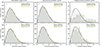 |
Fig. A.2. Same as Fig. A.1, but with the separation between eROSITA and LS10 counterparts by S25 in yellow. All matches with the LS10 counterpart catalog are shown in panels a and d. Panels b–f only show sources where S25 provides the same or a different counterpart, respectively. |
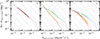 |
Fig. A.3. log N-log S distributions of different BlazEr1 subsamples, same as Fig. 14, but for the eROSITA main band and including the fit results listed in Table 5. The color scheme is the same as in Fig. 14. The red line in the left panel shows the best fit broken power law for the entire sample (α1 = 1.003 ± 0.013, α2 = 1.39 ± 0.07, FX, break, 0.2 − 2.3 keV = (2.11 ± 0.26)×10−12 erg cm−2 s−1, C = 30.6 ± 2.5 deg−2). |
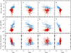 |
Fig. A.4. SED parameters from the 4LAC catalog as a function of various broadband spectral indices, following the color scheme introduced in Fig. 3. For the uncertainties of the parameters from the 4LAC we give the median uncertainty, when available, and in case of the Compton dominance by means of error propagation, as black data points in panels a and i. |
Appendix B: Supplemental tables
In this appendix, we present the tables summarizing the different correlations and the mean values of the broadband spectral indices. Table B.1 lists all kinds of different parameter combinations and the respective correlation values, while Table B.2 compares the broadband spectral indices with the SED parameters and Table B.3 lists correlation coefficients between the different broadband spectral indices. Mean values for the broadband spectral indices are given in Table B.4.
Correlation coefficients for various parameter combinations discussed throughout the paper.
Correlation coefficients for parameters α and SED parameters from the 4LAC catalog.
Correlation coefficients for parameters α.
Mean and standard deviation values for parameters of α.
Appendix C: The BLAZE catalogs
The BLAZE catalog is obtained by merging the catalogs listed in Table 1 with the respective merging radii (Sect. 2). The BLAZE catalog contains redshifts from these input catalogs. Based on eROSITA’s sensitivity and exposure, we are able to calculate flux and luminosity upper limits for all sources in the western Galactic hemisphere. The sources removed due to quality issues (see Sect. 2.2) are released as a separate file as well. The catalogs are released as FITS files with the following columns:
SRC_NAME: Common name of the source.
RAJ2000, DEJ2000: Equatorial coordinates from input catalog [°, J2000.0].
LII, BII: Galactic coordinates from input catalog [°].
BLAZAR_CLASS: Classification given by the input catalog.
Z: Redshift given in the input catalog.
Z_REF: Reference for the redshift.
ERO_EXPO: eROSITA exposure time at source position, if available [s].
ERO_UL_FLUX: Upper limit 0.2–2.3 keV flux, based on exposure time and sensitivity [erg cm−2 s−1].
ERO_UL_LUM: Upper limit for the 0.2–2.3 keV luminosity band based on ERO_UL_FLUX [erg cm−2 s−1].
REMOVE_FLAG: Only for the unverified BLAZE catalog, reason for removal: 1: HECATE, 2: Xie et al. (2024), 3: Rakshit et al. (2017), 4: Gordon et al. (2023), 5: known non-blazar.
Appendix D: The BlazEr1 catalogs
In the following we describe all 661 FITS columns of the BlazEr1 catalogs, that is, the unverified and the standard BlazEr1 catalog. As described in Sect. 3.1.1, these catalogs were obtained by merging various input catalogs, which are matched with the eRASS1 catalog (Merloni et al. 2024), and amending this list of sources with additional information such as, for example, spectral fit results. In the following the energy bands for X-ray and γ-ray fluxes and luminosities are denoted with n, where n is defined in Table D.1.
X-ray and γ-ray energy band designators used in the BlazEr1 catalog.
For the fluxes determined by fitting a power law with fixed photon index to the spectra we denote the photon index G used, as listed in Table D.2.
Photon index designators G for flux values
The LS10 bands (G, R, I, Z, W1, W2, W3, and W4) are denoted by X in the column names listed below. For RFC values the bands (s, c, x, u, and k) are denoted by Y. Not all parameters will have all of the bands available denoted with X. Where parameters have uncertainties, they are consistently listed in a column obtained by appending _ERR to the column name. For symmetric error bars the column is a standard FITS column, asymmetric confidence intervals of the type  are given as fixed length arrays with two entries, −l and +u, including the sign. Sometimes symmetric and asymmetric uncertainties are given, since some methods return asymmetric uncertainties which then are approximately summarized as symmetric ones (_ERR, _ASYM_ERR). In the online Vizier version the asymmetric uncertainties are given as two columns which are prefixed by E_ and e_ for upper and lower uncertainties, respectively. Overall, column names might slightly vary in the Vizier version. Unless noted otherwise, confidence intervals are given at the 1σ confidence level, except for spectral parameters (e.g., photon indices, fluxes), where 90% confidence intervals are given, following the conventions of X-ray astronomy. Sometimes the inverse variance (_IVAR) is given instead of an uncertainty. Where columns are taken from other catalogs, we sometimes copy in part the original column descriptions in verbatim.
SRC_NAME: Common name of the source.
RAJ2000, DECJ2000: Equatorial coordinates from input catalog [°].
BLAZAR_CLASS: Blazar classification given by the input catalog.
CONF_BLAZAR: 1 for confirmed blazars and 0 for candidates.
FGL_SRC_NAME: Name of source if listed in 4FGL (4FGL-DR4; Abdollahi et al. 2022).
BZCAT_SRC_NAME: Name of source if listed in BZCAT (Massaro et al. 2015).
HSP_SRC_NAME: Name of source if listed in 3HSP (Chang et al. 2019).
HIGHZ_SRC_NAME: Name of source if listed in the HighZ sample (Sbarrato et al. 2026)
MILLIQUAS_SRC_NAME: Name of source if listed in Milliquas (Flesch 2023).
KDEBLLACS_SRC_NAME: Name of source if listed in KDEBLLACS (D’Abrusco et al. 2019).
WIBRALS2_SRC_NAME: Name of source if listed in WIBRaLS2 (D’Abrusco et al. 2019).
ABC_SRC_NAME: Name of source if listed in ABC (Paggi et al. 2020).
BROS_SRC_NAME: Name of source if listed in BROS (Itoh et al. 2020).
ANGSEP: Angular separation between catalog and eROSITA position [°].
DETUID: eROSITA unique detection ID.
IAUNAME: Official IAU name of the eROSITA source.
SKYTILE: eROSITA sky tile ID.
ID_SRC: eROSITA source ID in each sky tile.
UID: Integer unique detection ID. See Merloni et al. (2024) for details.
UID_HARD: Hard catalog UID of the source with a strong association, or -UID if the association is weak. 0 means no counterpart found in the Hard catalog.
ID_CLUSTER: Group ID of sources simultaneously modeled during source detection.
RA(_ERR), DEC(_ERR): Equatorial coordinates and associated uncertainties of eROSITA source (ICRS) [°].
RA_RAW(_ERR), DEC_RAW(_ERR): Equatorial coordinates of eROSITA source (ICRS), without applying the eROSITA aspect correction [°].
POS_ERR: 1σ position uncertainty [″].
RADEC_ERR: Combined positional error, raw output from PSF fitting [″].
LII, BII: Galactic coordinates of eROSITA source with applied position correction (not identical to the coordinates listed by Merloni et al. 2024) [°].
ELON, ELAT: Ecliptic coordinates of eROSITA source [°].
MJD: Modified Julian Date of the observation of the source nearest to the optical axis of eROSITA.
MJD_MIN, MJD_MAX: Modified Julian Date of the sources’ first and last eROSITA observation.
EXT(_ERR , _ASYM_ERR): Source extent parameter and associated uncertainty [″].
EXT_LIKE: Extent likelihood.
DET_LIKE_n: Detection likelihood.
ML_CTS_n(_ERR , _ASYM_ERR): ML source net counts and associated uncertainty [cts].
ML_RATE_n(_ERR , _ASYM_ERR): ML source count rate and associated uncertainty [cts s−1].
ML_FLUX_n(_ERR , _ASYM_ERR): ML source flux and associated uncertainty [erg cm−2 s−1].
ML_BKG_n: ML background counts at the source position [(′)−2].
ML_EXP_n: ML vignetted exposure time at the source position [s].
ML_EEF_n: ML enclosed energy fraction.
APE_CTS_n: Total counts extracted within the aperture [cts].
APE_BKG_n: Background counts extracted within the aperture, excluding nearby sources using the source map [cts].
APE_EXP_n: Exposure map value at the given position [s].
APE_RADIUS_n: Extraction radius [pixel, 1 pixel corresponds to 4″].
APE_POIS_n: Poisson probability that the extracted counts (APE_CTS) are background fluctuation.
FLAG_SP_SNR: If 1, source may lie within an overdense region near a supernova remnant.
FLAG_SP_BPS: If 1, source may lie within an overdense region near a bright point source.
FLAG_SP_SCL: If 1, source may lie within an overdense region near a stellar cluster. FLAG_SP_LGA: If 1, source may lie within an overdense region near a local large galaxy.
FLAG_SP_GC_CONS: If 1, source may lie within an overdense region near a galaxy cluster.
FLAG_NO_RADEC_ERR: If 1, source contained no RA_DEC_ERR in the preprocessed version of the catalog.
FLAG_NO_EXT_ERR: If 1, source contained no EXT_ERR in the preprocessed version of the catalog.
FLAG_NO_CTS_ERR: If 1, source contained no ML_CTS_0_ERR in the preprocessed version of the catalog.
FLAG_OPT: If 1, source matched within 15″ with a bright optical star, likely contaminated by optical loading.
CTS_n_(_ERR): Counts from spectrum and associated uncertainty (Gehrels 1986) [cts].
SPEC_EXPOTIME: Exposure time as given in the spectrum [s].
EXPOTIME: Exposure time from the eROSITA exposure map for the 0.2–2.3 keV band [s].
MIN_FLUX_95: Minimum detectable flux at source position to guarantee 95% detection rate with a DET_LIKE_0 of 10 or greater in the 0.2–2.3 keV band [erg cm−2 s−1].
AVERAGE_NH: Average N H from the HI4PI Collaboration (2016) [cm−2].
WE_AVERAGE_NH: Weighted average N H from the HI4PI Collaboration (2016) [cm−2].
HR12(_ERR): Hardness ratio between 0.2–0.7 keV and 0.7–1.2 keV and associated uncertainty.
HR23(_ERR): Hardness ratio between 0.7–1.2 keV and 1.2–2.3 keV and associated uncertainty.
HR13(_ERR): Hardness ratio between 0.2–0.7 keV and 1.2–2.3 keV and associated uncertainty.
PWLG_NORM(_ERR): Power law norm using a fixed N H and an index of G at 1 keV and associated uncertainty [photons keV−1 cm−2 s−1].
PWLG_FLUX_(UNABS , ABS)_n(_ERR): Fitted unabsorbed and observed flux using a fixed N H and fixed power law index G and associated uncertainty [erg cm−2 s−1].
PWLG_C_VARIANCE: Variance of Cash statistics of fixed N H and fixed power law index fit according to Kaastra (2017).
PWLG_CASH: Cash statistics of fixed N H and fixed power law index fit.
PWLG_CSTAT_THEORY: Theoretical Cash statistics while using a fixed N H and fixed power law index fit according to Kaastra (2017).
PWLG_REDCASH: Reduced Cash statistics from fit with fixed N H and fixed power law index.
PWLG_CASHBINS: Number of bins used during the fixed N H and fixed power law index fit.
PWLG_CASHPAR: Number of parameters used during the fixed N H and fixed power law index fit.
PWLG_NUM_BINS: Number of bins used to calculate Kaastra (2017) values of fixed N H and fixed power law index.
Flux_JY(_ERR): Flux density at 1 keV derived from the norm of the fixed Γ X = 2.0 fit [Jy].
(FREE_ , FIXED_)NH(_ERR): Freely fitted or fixed N H and associated uncertainty [cm−2].
(FREE_ , FIXED_)GAMMA(_ERR): Power law photon index using a free or fixed N H and associated uncertainty.
(FREE_ , FIXED_)NORM(_ERR): Power law norm using a free or fixed N H at 1 keV and associated uncertainty [photons keV−1 cm−2 s−1].
(FREE_ , FIXED_)FLUX_(UNABS , ABS)_n(_ERR): Fitted unabsorbed and observed flux for a free or fixed N H power law fit and associated uncertainty [erg cm−2 s−1].
(FREE_ , FIXED_)C_VARIANCE: Variance of Cash statistics of free or fixed N H power law fit according to Kaastra (2017).
(FREE_ , FIXED_)CASH: Cash statistics of free or fixed N H power law fit.
(FREE_ , FIXED_)CSTATS_THEORY: Theoretical Cash statistics while using a free or fixed N H power law fit according to Kaastra (2017).
(FREE_ , FIXED_)REDCASH: Reduced Cash statistics from fit with free or fixed N H.
(FREE_ , FIXED_)CASHBINSs: Number of bins used during the free or fixed N H power law fit.
(FREE_ , FIXED_)CASHPAR: Number of parameters used during the free or fixed N H power law fit.
(FREE_ , FIXED_)NUM_BINS: Number of bins used to calculate Kaastra (2017) values of free or fixed N H power law fit.
RXS_RA , RXS_DEC: Equatorial position of 2RXS source (Boller et al. 2016) [°].
RXS_NH_GAL: Galactic N H assumed by Boller et al. (2016) [cm−2].
RXS_NH: N H derived from fit by Boller et al. (2016) [cm−2].
RXS_GAMMA(_ERR): Γ X from fit and associated uncertainty by Boller et al. (2016).
RXS_FLUX_n: Flux from power law fit by Boller et al. (2016) [erg cm−2 s−1].
XRT_SRC_NAME: Name given in Evans et al. (2020).
XRT_RA, XRT_DEC: Equatorial coordinates from Evans et al. (2020) [°].
XRT_XRT_ANGSEP: Angular separation between blazar catalog source and closest source in Evans et al. (2020) [″].
XRT_FLAG: If 1 the blazar and the source listed by Evans et al. (2020) are located within 8″ of each other.
XRT_NH(_ERR): Galactic NH and associated uncertainty from Evans et al. (2020) [cm−2].
XRT_GAMMA(_ERR): Power law photon index and associated uncertainty from Evans et al. (2020).
XRT_(ABS , UNABS)_FLUX_n(_ERR): Unabsorbed and observed flux and associated uncertainty from Evans et al. (2020) [erg cm−2 s−1].
OUSXB_RA, OUSXB_DEC: Equatorial coordinates of Swift-XRT sources from Giommi et al. (2019) [°].
OUSXB_(MIN, MAX, MEAN, MEDIAN)_FLUX_n: Minimum, maximum, median and mean sources flux from (Giommi et al. 2019) [erg cm−2 s−1].
OUSXB_N_FLUX_n: Number of observations of source in Giommi et al. (2019) with a flux.
OUSXB_(MIN, MAX, MEAN, MEDIAN)_GAMMA: Minimum, maximum, median and mean power law photon index (Giommi et al. 2019).
OUSXB_N_GAMMA: Number of observations of source in Giommi et al. (2019) with a power law photon index.
NUSTAR_RA, NUSTAR_DEC: Equatorial coordinates of NuSTAR sources from Middei et al. (2022) [°].
NUSTAR_GAMMA(_ERR): Photon index of NuSTAR sources from Middei et al. (2022).
NUSTAR_FLUX_n(_ERR): Flux of NuSTAR sources from Middei et al. (2022) [erg cm−2 s−1].
BAT_SRC_NAME: Name of source given by Lien et al. (2025).
BAT_RA, BAT_DEC: Equatorial coordinates of Swift-BAT sources from Lien et al. (2025) [°].
BAT_TYPE: Source type provided by Lien et al. (2025).
BAT_( , MIN_ , MAX_)FLUX_n: Flux, minimum and maximum flux of Swift-BAT sources from Lien et al. (2025) [erg cm−2 s−1].
BAT_( , MIN_ , MAX_)GAMMA: Photon index of Swift-BAT sources from Lien et al. (2025).
ASCAMASTER_EXPOTIME: ASCA exposure time according to Heasarc’s ascamaster table [s].
CHANMASTER_EXPOTIME] Chandra exposure time according to the chanmaster table [s].
NUMASTER_EXPOTIME: NuSTAR exposure time according to the numaster table [s].
SUZAMASTER_EXPOTIME: Suzaku exposure time according to the suzamaster table [s].
XMMMASTER_EXPOTIME: XMM-Newton exposure time according to the xmmmaster table [s].
SWIFTMASTR_EXPOTIME: Swift-XRT exposure time according to the swiftmastr table in [s].
ROSMASTER_EXPOTIME: ROSAT exposure time according to the rosmaster table in [s].
FGL_COMMON_SRC_NAME: Name of identified or likely associated source from the 4FGL catalog (4FGL-DR4; Abdollahi et al. 2022).
FGL_FLUX_n(_ERR): Integral photon flux and associated uncertainty for the B band (4FGL-DR4; Abdollahi et al. 2022) [photons cm−2 s−1].
FGL_FLUX_n(_ERR): Energy flux and associated uncertainty for the A band (4FGL-DR4; Abdollahi et al. 2022) [erg cm−2 s−1].
FGL_SPEC_TYPE: Spectral type in the global model (Power Law, LogParabola, PLSuperExpCutoff) (4FGL-DR4; Abdollahi et al. 2022).
FGL_PL_FLUXDEN(_ERR): Differential flux at pivot energy of the power law fit and associated uncertainty (4FGL-DR4; Abdollahi et al. 2022) [cm−2 MeV−1 s−1].
FGL_PL_INDEX(_ERR): Photon index of power law fit and associated uncertainty (4FGL-DR4; Abdollahi et al. 2022).
FGL_LP_FLUXDEN(_ERR): Differential flux at pivot energy of the LogPar fit and associated uncertainty (4FGL-DR4; Abdollahi et al. 2022) [cm−2 MeV−1 s−1].
FGL_LP_INDEX(_ERR): Photon index at pivot energy for LogPar fit and associated uncertainty (4FGL-DR4; Abdollahi et al. 2022).
FGL_LP_BETA(_ERR): Curvature parameter of LogPar fit and associated uncertainty (4FGL-DR4; Abdollahi et al. 2022).
FGL_LP_EPEAK(_ERR): Peak energy of LogPar fit and associated uncertainty (4FGL-DR4; Abdollahi et al. 2022) [MeV].
FGL_LP_SIGCURV: Significance of fit improvement between Power Law and LogParabola (4FGL-DR4; Abdollahi et al. 2022) [σ].
FGL_PLEC_FLUXDEN(_ERR): Differential flux at pivot energy of the PLSuperExpCutoff fit and associated uncertainty (4FGL-DR4; Abdollahi et al. 2022) [cm−2 MeV−1 s−1].
FGL_PLEC_INDEX(_ERR): Photon index at pivot energy for PLSuperExpCutoff fit and associated uncertainty (4FGL-DR4; Abdollahi et al. 2022).
FGL_PLEC_EXPFACTOR(_ERR): Spectral curvature at pivot energy for PLSuperExpCutoff fit and associated uncertainty (4FGL-DR4; Abdollahi et al. 2022).
FGL_PLEC_EXPINDEX(_ERR): Exponential index of PLSuperExpCutoff and associated uncertainty (4FGL-DR4; Abdollahi et al. 2022).
FGL_PLEC_EPEAK(_ERR): Peak energy of PLSuperExpCutoff fit and associated uncertainty (4FGL-DR4; Abdollahi et al. 2022) [MeV].
FGL_PLEC_SIGCURV: Significance of fit improvement between Power Law and PLSuperExpCutoff (4FGL-DR4; Abdollahi et al. 2022) [σ].
LAC_SED_CLASS: SED classes listed in the 4LAC catalog by Ajello et al. (2022).
LAC_HE_EPEAK(_ERR): High-energy peak position listed in the 4LAC catalog by Ajello et al. (2022) and associated uncertainty [MeV].
LAC_HE_NUFNU(_ERR): High-energy peak flux listed in the 4LAC catalog by Ajello et al. (2022) [MeV cm−2s−1].
LAC_LE_FREQ: Low-energy peak position listed in the 4LAC catalog by Ajello et al. (2022) [Hz].
LAC_LE_NUFNU: Low-energy peak flux listed in the 4LAC catalog by Ajello et al. (2022) [erg cm−2 s−1].
RFC_SRC_NAME: Name of source in RFC catalog (Petrov & Kovalev 2025).
RFC_YBAND_RES: Total Y-band flux density integrated over entire map (Petrov & Kovalev 2025) [Jy].
RFC_YUPPER_RES: Blank for valid Y-band resolved total flux density, − for invalid and < for upper limits (Petrov & Kovalev 2025).
RFC_YBAND_UNRES: Unresolved Y-band flux density at long VLBA baselines (Petrov & Kovalev 2025) [Jy].
RFC_YUPPER_UNRES: Blank for valid Y-band unresolved flux density at VLBA baselines, − for invalid and < for upper limits (Petrov & Kovalev 2025).
TANAMI_SRC_NAME: Name within TANAMI program (Ojha et al. 2010; Müller et al. 2018).
TANAMI_CLASS: Class given by TANAMI (Ojha et al. 2010; Müller et al. 2018).
TANAMI_FLUX: Flux density at 8.4 GHz from TANAMI (Ojha et al. 2010; Müller et al. 2018) [Jy].
MOJAVE_SRC_NAME: Name of source in the MOJAVE program (Lister et al. 2021; Homan et al. 2021).
MOJAVE_CLASS: Class as listed by MOJAVE (Lister et al. 2021; Homan et al. 2021) (Q or B).
MOJAVE_FLUX: Flux density at 15 GHz from MOJAVE (Lister et al. 2021; Homan et al. 2021) [mJy].
N_MATCH: Number of potential counterparts (S25).
LS10_sep: Angular separation between BLAZE catalog and LS10 source [″].
LS10_use: 1 for agreement on the counterpart with S25, 0 otherwise.
LS10_RELEASE: LS10 release of counterpart (S25).
LS10_BRICKID: LS10 brick ID of counterpart (S25).
LS10_OBJID: LS10 object ID of counterpart (S25).
LS10_RA(_IVAR) , LS10_DEC(_IVAR): Position of LS10 counterpart (S25) [° , ( ° )−2].
LS10_Xray_proba: Probability of LS10 counterpart being an X-ray emitter (S25).
LS10_FULLID: LS10 catalog ID (S25).
ERO_LS10_ID: Combined eROSITA and LS10 catalog ID (S25).
Separation_LS10_ERO: Separation between LS10 counterpart and eROSITA position (S25) [″].
NCAT: Number of catalogs matched (S25).
DIST_BAYESFACTOR: Logarithm of ratio from prior and posterior distance matching (S25).
DIST_POST: Distance between posterior probability of a match compared to no matches (S25).
BIAS_LS10_XRAY_PROBA: Probability of counterpart being an X-ray emitter (S25).
P_SINGLE: Similar to DIST_POST including weighting by prior (S25).
P_ANY: Probability of any found match being correct (S25).
P_I: Match probability (S25).
MATCH_FLAG: Set to 1 for most probable match, 2 for other matches (S25).
TYPE: LS10 morphology model given by S25.
LS10_DCHISQ: Difference in χ 2 between successively more-complex model fits separated by _ (S25).
EBV: E(B − V) at source position (S25) [mag] .
FLUX(_IVAR)_X: LS10 band fluxes and associated inverse variance (S25) [nanomaggy , nanomaggy−2].
MW_TRANSMISSION_X: LS10 Galactic transmission at position of source (S25).
ANYMASK_X: Bitmask information if in any image of a band the central pixel satisfies the LS10 catalog criteria (S25).
ALLMASK_X: Bitmask information if in all image of a band the central pixel satisfies the LS10 catalog criteria (S25).
PSFSIZE_X: Size of FWHM of the LS10 PSF (S25) [″].
PSFDEPTH_X: LS10 5σ detection limit for a certain band (S25) [nanomaggy−2].
GALDEPTH_X: Same as PSFSIZE_X assuming a galaxy (S25) [nanomaggy−2]. WISEMASK_X: Bitmask information (S25).
W(1 , 2 , 3 , 4)_MAG_AB: WISE magnitude in AB system calculated from FLUX_X using MW_TRANSMISSION_X [mag].
W(1 , 2 , 3 , 4)_MAG: WISE magnitude in the Vega system calculated from FLUX_X using MW_TRANSMISSION_X [mag].
SHAPE_R(_IVAR): LS10 half-light radius for given TYPE (S25) [″ , ″−2]. SHAPE_(E1 , E2)(_IVAR): LS10 ellipticity component of galaxy (S25).
SERSIC(_IVAR): LS10 power law index of Sérsic profile and associated inverse variance (S25).
REF_CAT: LS10 reference catalog for stars (S25).
REF_ID: LS10 reference catalog id for star (S25).
REF_EPOCH: LS10 reference epoch of REF_CAT (S25) [a].
GAIA_PHOT_G_MEAN_MAG: LS10 Gaia G band magnitude (S25) [mag].
GAIA_PHOT_G_MEAN_FLUX_OVER_ERROR: LS10 Gaia G band signal-to-noise ratio (S25).
GAIA_PHOT_BP_MEAN_MAG: LS10 Gaia BP band magnitude (S25) [mag].
GAIA_PHOT_BP_MEAN_FLUX_OVER_ERROR: LS10 Gaia BP band signal-to-noise ratio (S25).
GAIA_PHOT_RP_MEAN_MAG: LS10 Gaia RP band magnitude (S25) [mag].
GAIA_PHOT_RP_MEAN_FLUX_OVER_ERROR: LS10 Gaia RP band signal-to-noise ratio (S25).
GAIA_ASTROMETRIC_EXCESS_NOISE: LS10 Gaia astrometric excess noise (S25).
GAIA_PHOT_BP_RP_EXCESS_FACTOR: LS10 Gaia BP/RP excess factor (S25).
GAIA_ASTROMETRIC_SIGMA5D_MAX: LS10 Gaia longest semi-major axis of the 5-d error ellipsoid (S25).
GAIA_DUPLICATED_SOURCE: LS10 Gaia duplicate source flag (S25).
INALLLS10: Nominal LS10 survey depth reached in all bands (S25).
INANYLS10: Nominal LS10 survey depth reached in one band (S25).
DERED_MAG_X: Dereddend magnitude (S25) [mag].
SOFTFLUX_S: eROSITA flux (S25) [erg cm−2 s−1].
SALVATO18_W1_X_LINEDISTANCE: Distance from separation line between Galactic and extra-galactic sources in the W1-X-ray plane (S25).
SALVATO22_ZW1_GR_LINEDISTANCE: Distance from separation line between Galactic and extra-galactic sources in the ZW1-GR plane (S25).
(G , Z , W1)_MINUS_(R , W1 , W2): Color combinations (S25) [mag].
HAS_SALVATO18_AGN_COLORS: Information if source has colors consistent with being an AGN based on Salvato et al. (2018), from S25.
GAIA_MOVING_5SIGMA: Information if source shows movement at 5σ significance in Gaia (S25).
HAS_SALVATO22_AGN_COLORS: Information if source has colors consistent with being an AGN based on Salvato et al. (2022), from S25.
SALVATO_MAIN_ID_SIMBAD: SIMBAD ID (S25).
SALVATO_(RA , DEC)_SIMBAD: SIMBAD position (S25) [°].
EXGAL_PROB_STAREX: Probability of source being extra-galactic by STAREX with Gaia data (S25).
EXGAL_PROB_STAREX: Probability of source being extra-galactic by STAREX without Gaia data (S25).
CLASS_GAL_EXGAL: Galactic/extra-galactic class assigned by S25.
SALVATO_HECATE: 1 for sources within HECATE source (S25) [°].
SALVATO_HEC_OBJNAME: Name of HECATE source (S25).
SALVATO_HEC_RA , SALVATO_HEC_DEC: Position of HECATE source (S25) [°].
SALVATO_HEC_R1: Semi major axis of HECATE source (S25) [′].
SALVATO_HEC_R2: Semi minor axis of HECATE source (S25) [′].
SALVATO_HEC_PA: Position angle of HECATE source (S25) [°].
PURITY(6 , 7 , 8): Purity obtained for DET_LIKE_0 > (6, 7, 8) at source position (S25).
COMPLETENESS(6 , 7 , 8): Completeness obtained for DET_LIKE_0 > (6, 7, 8) at source position (S25).
COMPUR(6 , 7 , 8): Intersection between completeness and purity obtained for DET_LIKE_0 > (6, 7, 8) at source position (S25).
THRESHOLD(6 , 7 , 8): P_ANY value at intersection obtained for DET_LIKE_0>(6 , 7 , 8) at source position (S25).
Z_PHOTO(_S3L , _S3U , _S1L , _S1U): 3σ and 1σ upper and lower value of photometric redshift (S25).
Z_SPEC: Spectroscopic redshift from Kluge et al. (2024) provided by S25.
SPEC_REF: Source with Z_SPEC from Kluge et al. (2024) provided by S25.
Z_ABC: Redshift listed in the ABC catalog (Paggi et al. 2020).
Z_HSP: Redshift listed in the 3HSP catalog (Chang et al. 2019).
Z_F_HSP: Redshift flag listed in the 3HSP catalog (Chang et al. 2019).
Z_MILLIQUAS: Redshift listed in the Milliquas catalog (Flesch 2023).
Z_HIGHZ: Redshift listed in the HighZ sample.
Z_HIGHZ_REF: Paper reference for high-redshift sources.
Z_MOJAVE: Redshift listed in MOJAVE.
Z_4LAC: Redshift listed in the 4LAC catalog (Ajello et al. 2022).
Z_BZCAT: Redshift listed from the BZCAT catalog (Massaro et al. 2015).
Z_U_BZCAT: Redshift flag from the BZCAT catalog (Massaro et al. 2015).
Z_CGRABS: Redshift listed in the CGRaBS catalog (Healey et al. 2008).
Z_F_CGRABS: Redshift flag listed in CGRaBS catalog (Healey et al. 2008).
Z_VERONCAT: Redshift listed in the VERONCAT catalog (Véron-Cetty & Véron 2010).
Z_VERONCAT_QSO: Redshift listed in the VERONCAT QSO catalog (Véron-Cetty & Véron 2010).
Z_SIMBAD: Redshift listed on SIMBAD.
Z_MASTER: Reliable redshift adopted for population studies (for selection see Sect. 4.4).
Z_MASTER_REF: Source of Z_MASTER.
Z_MASTER_PHOTO: Reliable redshift including the photometric ones from S25.
Z_MASTER_PHOTO_REF: Source where Z_MASTER_PHOTO was taken from.
XRAY_LUM_n(_ERR): X-ray luminosity calculated from the fixed Γ X = 2.0 fit and Z_MASTER [erg s−1].
XRAY_LUM_PHOTO_n(_ERR): X-ray luminosity calculated from the fixed Γ X = 2.0 fit and Z_MASTER_PHOTO [erg s−1].
alpha_XG(_ERR): α XΓ using PWL20_FLUX_UNABS_0 and FGL_FLUX_A and associated uncertainty.
alpha_IRX(_ERR): α IRX using PWL20_FLUX_UNABS_0 and FLUX_W1 combined with MW_TRANSMISSION_W1 and associated uncertainty, including a systematic uncertainty.
alpha_OX(_ERR): α OX using PWL20_FLUX_UNABS_0 and FLUX_R combined with MW_TRANSMISSION_R and associated uncertainty, including a systematic uncertainty.
alpha_RX(_ERR): α RX using PWL20_FLUX_UNABS_0 and RFC_XBAND_RES and associated uncertainty.
alpha_TANAMI(_ERR): α TANAMI using PWL20_FLUX_UNABS_0 and TANAMI_FLUX and associated uncertainty.
alpha_MOJAVE(_ERR): α MOJAVE using PWL20_FLUX_UNABS_0 and MOJAVE_FLUX and associated uncertainty.
SIMBAD_SRC_NAME: Name of closest source match on SIMBAD.
SIMBAD_TYPE: Type of source, if a blazar or AGN classification or a more precise type is listed as alternative, this one is selected.
SIMBAD_ALT_TYPES: All alternate types as listed in SIMBAD.
SIMBAD_TYPE2: Type of source as listed by SIMBAD.
SIMBAD_ANGSEP: Angular separation between BLAZE catalog source and SIMBAD source [°]
CAMBRIDGE_SRC_NAME: Name in Third Cambridge catalog of radio sources as listed in SIMBAD.
PARKS_SRC_NAME: Name in Parkes catalog of radio sources as listed in SIMBAD.
TEXAS_SRC_NAME: Name in Texas survey of radio sources as listed in SIMBAD.
EINSTEIN_SRC_NAME: Name in Einstein 2E catalog of IPC X-Ray sources as listed in SIMBAD.
COMMON_SRC_NAME: Most commonly used source name from the above as listed in SIMBAD.
BZCAT_RMAG: R-band magnitude from the BZCAT catalog (Massaro et al. 2015) [mag].
BZCAT_FR: Radio flux density at 1.4 GHz or if unknown at 0.843 GHz from the BZCAT catalog (Massaro et al. 2015) [mJy].
BZCAT_F143: Flux density at 143 GHz from the Planck Compact Source Catalog Public Release 1 from the BZCAT catalog (Massaro et al. 2015) [mJy].
BZCAT_FLUX_U: X-ray flux in the 0.1–2.4 keV band from the BZCAT catalog (Massaro et al. 2015) [fWm−2].
BZCAT_FLUX_B: γ-ray flux in the 1–100 GeV band from the BZCAT catalog (Massaro et al. 2015) [photons cm−2 s−1].
BZCAT_ALPHA_RO: The radio-to-optical spectral index of the blazar from the BZCAT catalog (Massaro et al. 2015).
XIE_MORPH_BZCAT: Radio morphology for BZCAT sources as listed in Xie et al. (2024).
XIE_MORPH_KDEBLLACS: Radio morphology for KDEBLLACS sources as listed in Xie et al. (2024).
XIE_MORPH_WIBRALS: Radio morphology for WIBRaLS sources as listed in Xie et al. (2024).
All Tables
Breakdown of the blazar source classes during the construction of the BlazEr1 catalog.
Correlation coefficients for various parameter combinations discussed throughout the paper.
Correlation coefficients for parameters α and SED parameters from the 4LAC catalog.
All Figures
|
Fig. 1. All-sky distribution of the BLAZE catalog gold sample (confirmed blazars) in Galactic coordinates (BLL: 1697, FSRQ: 1937, BCU: 2503, BZG: 164). The different blazar classes are shown color coded and with different symbols. |
| In the text | |
|
Fig. 2. Histograms of angular separation between BLAZE catalog and eROSITA positions (green) with the distribution of the matched eROSITA source positional uncertainty overlaid (yellow). The vertical line at 8″ indicates the distance threshold for the final sample. The cumulative distribution of the angular separation is shown in blue. a Sample of eROSITA observed blazars with 93% of the matches found within 8″, and 55% and 79% within 3″ and 5″, respectively. b eROSITA observed blazar candidates. Only 81% of matches are within 8″, and 31%/58% within 3″/5″. We show Rayleigh distributions (black) for illustrative purposes, calculated following Merloni et al. (2024, Eq. (3), assuming F = 0.8). |
| In the text | |
|
Fig. 3. Positions of the BlazEr1 sources in Galactic coordinates. The different colors and symbols indicate the blazar types in the catalog. Candidates, especially BCUCs, dominate the sample. The overdensity along l ∼ 240° coincides with the footprint of BROS. Confirmed blazars are displayed by filled symbols, candidates are shown in the same color without filling. All the following figures will adapt the same color and symbol scheme. |
| In the text | |
|
Fig. 4. Sky area in which 95% of all sources above a minimum flux will be detected with DET_LIKE_0 ≥10. The dashed line indicates the total area of the western Galactic hemisphere. The red line displays the sensitivity over the entire western Galactic hemisphere, while the blue line shows the extragalactic sky excluding an area of 15° below and above the Galactic plane and regions with radii of 5.5° around the Large Magellanic cloud (LMC) and 3.0° around the Small Magellanic cloud (SMC). |
| In the text | |
|
Fig. 5. Spectral fits of an absorbed power law model for three confirmed blazars with different fluxes. For 5BZQ J0547−6728, no prior X-ray observations are available. The three lower panels display the fit residuals for each source. Data from TM5 and 7 are displayed in a lighter color. |
| In the text | |
|
Fig. 6. Distribution of source counts with its cumulative distribution shown by the solid line curve. The dashed vertical line marks the threshold of 50 counts, above which we deem a spectral analysis meaningful. Only 20% of all sources are above this limit, while about half have fewer than 20 counts, as shown by the cumulative distribution (blue). |
| In the text | |
|
Fig. 7. Flux distribution in the BlazEr1 catalog. The majority of sources have fluxes below the survey completeness limit on the western Galactic hemisphere, the vertical line marks this limit. The cumulative distribution is shown in blue. |
| In the text | |
|
Fig. 8. Redshift distribution of BlazEr1 sources. The colors represent different subtypes. All BlazEr1 entries are shown in green (3627 sources), BLLs in blue, and FSRQs in orange. The inset shows the distribution for sources with z > 3.5. |
| In the text | |
|
Fig. 9. X-ray luminosity as a function of redshift. The different dashed lines display luminosities of sources with ΓX = 2.0 for increasing z and a fixed X-ray flux: from top (dashed line) to bottom (dash-double dot line), we display FX, 0.2 − 2.3 keV from 10−11 erg cm−2 s−1 down to 10−14 erg cm−2 s−1 in steps of 10. We show the main band eROSITA luminosity in panel a, following the color scheme introduced in Fig. 3; and the 2–10 keV X-ray luminosity in panel b. In gray the BlazEr1 sample is shown. Orange points are based on NuSTAR data (Middei et al. 2022), blue points on Swift-BAT (Marcotulli et al. 2022), using the redshifts from BZCAT and 3HSP for the NuSTAR and the redshifts from Marcotulli et al. (2022) and adopting their best fit models. |
| In the text | |
|
Fig. 10. Luminosity distribution for all sources with reliable redshifts. The panels show distributions for different subgroups of the eROSITA blazars and eROSITA blazar candidates, with vertical lines indicating the median luminosity for each subgroup (see Table 3). |
| In the text | |
|
Fig. 11. Scatter plot of hardness ratios between energy bands 1 (0.2–0.7 keV), 2 (0.7–1.2 keV), and 3 (1.2–5.0 keV). Sources with ≥50 counts are shown in the color scheme of Fig. 3, fainter sources in gray. These sources show a higher dispersion and larger uncertainties. Dotted lines show, from top to bottom, expected hardness ratios for photon indices ΓX = 1.0, ΓX = 2.0, and ΓX = 3.0. The absorption increases along the tracks toward the top-right corner. The majority of source hardnesses are consistent with power law spectra in the expected range of spectral shapes due to the large uncertainties. The black data point in the top-left corners displays the median uncertainties of all, including the low count sources. |
| In the text | |
|
Fig. 12. Probability distribution of photon indices for different types of eROSITA observed blazars and blazar candidates. The distribution takes into account the uncertainties of individual measurements of the photon index. |
| In the text | |
|
Fig. 13. Photon index as a function of a flux and b luminosity, following the color scheme introduced in Fig. 3 (BLL(C)s: blue, FSRQ(C)s: red, BCU(C)s: orange). |
| In the text | |
|
Fig. 14. log N-log S distributions for sources within the extragalactic sky. Panel a: comparison of the total sample of eROSITA observed blazars and blazar candidates (black) with the distribution by Giommi & Padovani, (2015, purple). Green and brown show the log N-log S for both classes separately (green: eROSITA observed blazars, brown: observed candidates). Panel b: comparison of the predictions of Giommi & Padovani (2015) for BLLs (light blue) and FSRQs (light red) with eROSITA measurements for BLLs, FSRQs, and BCUs, using the color code of Fig. 3). |
| In the text | |
|
Fig. 15. Swift-XRT flux reported by Giommi et al. (2019) as a function of eROSITA flux, following the color scheme introduced in Fig. 3. The mean values of all measurements for a source listed in Giommi et al. (2019) are shown. The uncertainties of the Swift-XRT fluxes represent the minimum and maximum values provided by Giommi et al. (2019). The solid line represents the unity line, while the dashed ones indicate a factor 10 difference between the measurements. |
| In the text | |
|
Fig. 16. Mean photon indices derived by Swift-XRT using Giommi et al. (2019) and eROSITA, following the color scheme introduced in Fig. 3. The uncertainties of the Swift-XRT photon indices represent the minimum and maximum values provided by Giommi et al. (2019). The solid line represents unity. Differences are observed, indicating that blazars are variable in their spectral properties. |
| In the text | |
|
Fig. 17. Fermi-LAT fluxes (4FGL-DR4; Abdollahi et al. 2022) compared with eROSITA fluxes. The three panels show the different subtypes, following the color scheme introduced in Fig. 3 (a: FSRQs, b: BLLs, c: BCUs). The Fermi-LAT uncertainties are scaled to match the confidence limit of the eROSITA data. |
| In the text | |
|
Fig. 18. Fermi-LAT photon index (4FGL-DR4; Abdollahi et al. 2022) compared with the eROSITA photon index, following the color scheme introduced in Fig. 3 (BLLs: blue, FSRQs: red, BCUs: orange). In solid, the linear best fit is shown, additionally the correlation between the two parameters found by Yuan & Fan (2014; dashed) and Fan et al. (2012; dotted) are displayed. The uncertainties of Γγ are extrapolated to the 90% confidence interval. |
| In the text | |
|
Fig. 19. Correlation of radio flux densities and eROSITA fluxes, following the color scheme introduced in Fig. 3, using a data from the TANAMI program, b data from MOJAVE, and c X-band flux densities from the RFC catalog. |
| In the text | |
|
Fig. 20. WISE color-color diagram, following the color scheme introduced in Fig. 3. Regions populated by different types of AGNs, as well as other objects, are shown. Compare our results to Salvato et al. (2018; Fig. 9), for a color-color diagrams of the 2RXS and XMMSL2 samples. |
| In the text | |
|
Fig. 21. Different photometric spaces combining optical, infrared and X-ray data, similar to Salvato et al. (2022; Fig. 18) for point sources detected in eFEDS, using the color scheme introduced in Fig. 3. Solid gray lines show positions usually occupied by quasars, whereas the gray dotted lines corresponded to Seyfert 2 galaxies. The dashed black lines in the top panels distinguish between Galactic and extragalactic sources. |
| In the text | |
|
Fig. 22. Broadband spectral indices αXΓ, αIRX, and αRX against each other, following the color scheme introduced in Fig. 3. Due to the similar values obtained for αOX and αIRX, the former is not shown here. |
| In the text | |
|
Fig. 23. X-ray luminosity as a function of redshift, following the color scheme introduced in Fig. 3. BlazEr1 sources are shown in gray. The colored symbols are sources with low DET_LIKE, quality issues or a high angular separation. The added lines are the same as in Fig. 9. The upper limits have been taken from the BLAZE catalog. |
| In the text | |
|
Fig. 24. Fermi-LAT flux as a function of eROSITA flux, following the color scheme introduced in Fig. 3. The gray points are BlazEr1 sources, whereas sources without a significant detection are shown in color. Arrows indicate the upper limits. |
| In the text | |
|
Fig. A.1. Histograms of the angular separation between the positions provided in the BLAZE catalog normalized by the respective eROSITA positional error. Top: eROSITA observed blazars. Bottom: eROSITA observed blazar candidates. Panels a and c: All the initial matches. Panels b and d: BlazEr1 sample with applied quality and separation cuts. The theoretical Rayleigh distributions are shown as a black solid line. |
| In the text | |
|
Fig. A.2. Same as Fig. A.1, but with the separation between eROSITA and LS10 counterparts by S25 in yellow. All matches with the LS10 counterpart catalog are shown in panels a and d. Panels b–f only show sources where S25 provides the same or a different counterpart, respectively. |
| In the text | |
|
Fig. A.3. log N-log S distributions of different BlazEr1 subsamples, same as Fig. 14, but for the eROSITA main band and including the fit results listed in Table 5. The color scheme is the same as in Fig. 14. The red line in the left panel shows the best fit broken power law for the entire sample (α1 = 1.003 ± 0.013, α2 = 1.39 ± 0.07, FX, break, 0.2 − 2.3 keV = (2.11 ± 0.26)×10−12 erg cm−2 s−1, C = 30.6 ± 2.5 deg−2). |
| In the text | |
|
Fig. A.4. SED parameters from the 4LAC catalog as a function of various broadband spectral indices, following the color scheme introduced in Fig. 3. For the uncertainties of the parameters from the 4LAC we give the median uncertainty, when available, and in case of the Compton dominance by means of error propagation, as black data points in panels a and i. |
| In the text | |
Current usage metrics show cumulative count of Article Views (full-text article views including HTML views, PDF and ePub downloads, according to the available data) and Abstracts Views on Vision4Press platform.
Data correspond to usage on the plateform after 2015. The current usage metrics is available 48-96 hours after online publication and is updated daily on week days.
Initial download of the metrics may take a while.