


| Issue |
A&A
Volume 709, May 2026
|
|
|---|---|---|
| Article Number | A277 | |
| Number of page(s) | 19 | |
| Section | Interstellar and circumstellar matter | |
| DOI | https://doi.org/10.1051/0004-6361/202555848 | |
| Published online | 25 May 2026 | |
Large Interstellar Polarisation Survey
III. Observational constraints on the structure of grains
1
European Southern Observatory,
Karl-Schwarzschild-Str. 2,
85748
Garching,
Germany
2
Armagh Observatory and Planetarium,
College Hill,
Armagh
BT61 9DG,
UK
3
National Chung Hsing University,
145 Xingda Rd.,
South Dist., Taichung City
402,
Taiwan
4
Tamkang University,
151 Yingzhuan Rd.,
Tamsui Dist., New Taipei City
251301,
Taiwan
5
Institut d’Astrophysique Spatiale, CNRS, Univ. Paris-Sud, Université Paris-Saclay,
Bât. 121, 91405 Orsay cedex,
France
6
Laboratoire Univers et Particules de Montpellier, Université de Montpellier,
CNRS/IN2P2, CC 72, Place Eugène Bataillon, 34095 Montpellier Cedex 5,
France
★ Corresponding author: This email address is being protected from spambots. You need JavaScript enabled to view it.
Received:
6
June
2025
Accepted:
30
March
2026
Abstract
Our understanding of dust in the diffuse interstellar medium remains incomplete with regard to the structure, composition, size distribution, and alignment properties of its grains. Joint observations of reddening, starlight polarisation spectra, and polarised dust emission for individual sightlines provide essential constraints on such properties. We studied a far-UV-selected sample of 96 reddening curves, for which optical linear polarisation spectra were obtained with FORS at the VLT as part of the Large Interstellar Polarisation Survey. Starlight polarisation spectra for 60 stars are presented in this work. These data are combined with Gaia distance estimates and Planck thermal dust emission. A three-component dust model is made publicly available. It consists of nanoparticles, amorphous grains, and micrometre-sized dust agglomerates, with varying axial ratios, porosities, sizes, element abundances, and alignment efficiencies that match observations. The diversity of reddening and polarisation spectra is well reproduced by prolate grains with typical axial ratios of two, a porosity of 10%, and high alignment efficiencies. Such efficiencies can be achieved with radiative torque alignment theory but not with imperfect Davis-Greenstein alignment, except when adjusting the magnetic-field orientation to maximise the polarisation. Micrometre-sized dust contributes wavelength-independent grey extinction in the optical and accounts for about one-third of the visual extinction and one-third of the dust mass. A follow-up sub-millimetre survey with high-resolution polarimetry will further constrain grain shapes and alignment physics.
Key words: dust, extinction
© The Authors 2026
 Open Access article, published by EDP Sciences, under the terms of the Creative Commons Attribution License (https://creativecommons.org/licenses/by/4.0), which permits unrestricted use, distribution, and reproduction in any medium, provided the original work is properly cited.
This article is published in open access under the Subscribe to Open model. This email address is being protected from spambots. You need JavaScript enabled to view it. to support open access publication.
1 Introduction
Dust is ubiquitous in the interstellar medium (ISM) and plays a significant role in many astrophysical processes. Clues as to the composition of interstellar dust come from various sources, such as observed elemental depletions in the gas phase and spectroscopic signatures of dust (Hensley & Draine 2021). The observed extinction curves display several spectral features, the most prominent being the 2175 Å bump, which is commonly attributed to graphite or polycyclic aromatic hydrocarbons (PAHs). Another important constraint is provided by dust emission, with conspicuous mid-IR emission bands often assigned to PAHs (Allamandola et al. 1989; Puget & Leger 1989). In addition, strong dust bands at 9.7 and 18 μm arise from the Si-O stretching and O-Si-O bending modes of silicate minerals, respectively (Dorschner et al. 1995). The extinction curve gives the dust extinction as a function of wavelength and provides strong constraints on dust models, in particular on the size distribution of the grains (Mathis et al. 1977).
The polarisation of starlight by dust extinction (Hall 1949; Hiltner 1949) and polarised thermal dust emission (Hildebrand 1988) show that interstellar dust grains are non-spherical and aligned with the interstellar magnetic field. This is the result of a rotating grain’s axis of maximum inertia (a) aligning with its angular momentum (J; i.e. internal alignment) and J aligning with the magnetic-field-line direction (B; i.e. external alignment). Internal alignment is generally believed to be driven by the Barnett effect (Purcell 1979). Theories suggested to explain external alignment include paramagnetic relaxation (the Davis-Greenstein effect; Davis & Greenstein 1951) and the torque exerted by an anisotropic radiation field on a helical grain due to the differential scattering/absorption of left-and right-handed circular polarisation (radiative torque theory; Dolginov & Mitrofanov 1976; Draine & Weingartner 1996; Lazarian 1997).
In the imperfect Davis-Greenstein (IDG) alignment (Hong & Greenberg 1980; Voshchinnikov 2012) the grain wobbles and rotates around its axis of greatest momentum while also precessing around the magnetic field vector. A major criticism pointed out by Jones & Spitzer (1967) and Roberge & Lazarían (1999) is that the Davis-Greenstein (DG) model ignores internal alignment and therefore is a physically incorrect simplification.
Following the development of an analytical model for radiative alignment theories (RATs; Lazarian & Hoang 2007), and due to its good qualitative agreement with polarimetric observations (e.g. Andersson et al. 2015), interest in RATs has increased significantly in the last two decades, and the original RAT has been significantly expanded. The high polarisation ceiling observed in dust thermal emission (∼20%; Planck Collaboration XIX 2015a) requires that dust grains be more efficiently aligned than either the DG effect or the RAT alignment in its original form can account for. A solution found by Hoang & Lazarian (2016) is to consider grains with iron inclusions, which results in increased grain magnetic susceptibility and, therefore, alignment: this is called the magnetically enhanced RAT (MRAT). MRAT successfully accounts for grain alignment from the diffuse ISM to dense star-forming regions (Giang et al. 2025). Note that while DG torques are also increased by iron inclusions, they are typically significantly weaker than MRAT torques.
In this study we correlated observational constraints with the physical properties of interstellar dust. We tested a dust model against representative element depletions, stellar distance estimates, and the characteristics of reddening and polarisation in absorption and, where available, in emission, along individual sightlines through the diffuse ISM. Particular attention was paid to micrometre-sized dust agglomerates that absorb a fraction of the interstellar radiation field (ISRF; Mathis et al. 1983; Bianchi 2024). Because they are large, they remain cold and emit at long wavelengths. Initially, very cold (10 K) dust emission was detected in our Galaxy towards high-density regions (Chini et al. 1993) and in non-active galaxies (Chini et al. 1995). This cold dust was later confirmed by Infrared Space Observatory (Krügel et al. 1998; Siebenmorgen et al. 1999). More recently, excess emission at 0.5 mm observed by Herschel could not be explained by a single modified blackbody temperature component (Madden et al. 2013; Kennicutt et al. 2011; Rémy-Ruyer et al. 2013), with similar results confirmed using ALMA (Galliano et al. 2005) and LABOCA (Galametz et al. 2009) at even longer wavelengths. Furthermore, micrometre-sized particles originating from the local interstellar cloud surrounding the Solar System’s ISM were directly measured in situ by the Ulysses, Galileo, and Stardust space probes (Landgraf et al. 2000; Westphal et al. 2014; Krüger et al. 2015). They appear in sightlines associated with the cold ISM (Siebenmorgen et al. 2020).
In the ISM, a grey component of micrometre-sized grains was introduced by Mathis et al. (1977) and Wang et al. (2015a,b) to account for the observed IR extinction. Such grains have also been incorporated into other dust models (Voshchinnikov 2004; Krügel & Siebenmorgen 1994; Krügel 2008; Ormel et al. 2011; Ysard et al. 2024). Recently, the impact of grey extinction on Type Ia supernova distance measurements was analysed by the Dark Energy Survey Collaboration (Popovic et al. 2024). The sub-millimetre excess continuum emission in the Milky Way detected by Planck (Planck Collaboration XII 2020) can be matched by adjusting the grain emissivity at these wavelengths (Hensley & Draine 2021). However, such models fail to resolve the discrepancy between trigonometric distance estimates provided by the Gaia Collaboration (2023) and the overprediction of the luminosity distance of the same stars (Siebenmorgen et al. 2025). Unification between luminosity and trigonometric distance estimates could be established by considering a population of micrometre-sized dust, which provides the necessary additional dimming of starlight. These grains are large enough to produce consistent reddening and grey extinction at wavelengths shorter than 1 μm.
For this purpose, the Large Interstellar Polarisation Survey (LIPS) was performed to measure the starlight polarisation spectra of 161 stars using the FORS instrument (Appenzeller et al. 1998) on the ESO Very Large Telescope (VLT). The observations covered a wavelength range of 0.38-0.95 μm at a spectral resolving power of ∼880. In Paper I (Bagnulo et al. 2017), a catalogue of 127 linear polarisation spectra corresponding to 101 sightlines was published.
2 The sample and data
Observing sightlines that intersect different components of the ISM introduces complexities in relating extinction and polarisation data to physical dust parameters. To address this issue, in Paper II (Siebenmorgen et al. 2018) stars were observed with the high-resolution spectrograph UVES, which offers a resolving power of λ/Δλ ~ 75 000 (Dekker et al. 2000; Smoker et al. 2009). These spectra were used to confirm the spectral type and luminosity class of the stars used for the reddening curve determination and to examine the profiles of interstellar absorption lines, particularly KI. The concept of ‘single-cloud sightlines’ was introduced, referring to cases where a dominant Doppler component accounts for more than half of the observed column density. A total of 65 such rare single-cloud sightlines were identified. It was found that interstellar polarisation is lower for multiple-cloud sightlines compared to single-cloud sightlines, indicating that the presence of additional clouds depolarises the transmitted radiation. Furthermore, significant variations in dust properties between different clouds were inferred from dust modelling.
In this work (Paper III), the sample is expanded with additional starlight polarisation spectra for 60 stars. The same observing strategy, data reduction, and calibration procedures as detailed in Paper I are applied (Bagnulo et al. 2017). Combining reddening and polarisation continuum observations is necessary to constrain the nature of interstellar dust, including its chemical composition and size distribution. For instance, the reddening rise in the far-UV is indicative of very small nanoparticles, and so is the 2175 Å bump (Stecher & Donn 1965; Blasberger et al. 2017), which is tied to carbonaceous nanoparticles. The shape of the polarisation curve in the optical (Serkowski et al. 1975) can be used to constrain the size distribution of aligned dust grains (Kim & Martin 1995; Vaillancourt et al. 2020).
The reddening curves have been derived in the near-IR (JHK) using the Two Micron All Sky Survey (2MASS; Cutri et al. 2003), in the optical (UBV) from ground-based facilities (Valencic et al. 2004), and in the far-UV below 0.3 μm down to the Lyman limit from space-based observations. At these short wavelengths, the International Ultraviolet Explorer (IUE) and the Far Ultraviolet Spectroscopic Explorer (FUSE) observed spectra for 417 stars (Valencic et al. 2004), 328 stars (Fitzpatrick & Massa 2007), and 75 stars with FUSE (Gordon et al. 2009). Furthermore, distances derived from Gaia parallaxes were used to estimate the reddening at infinite wavelength, providing an estimate of the visual extinction Av (Siebenmorgen et al. (2025), Eq. (21)).
The LIPS sample is further complemented by observations of polarised dust emission obtained from the Planck observatory at 850 μm (Planck Collaboration XII2020). The Planck total intensity and polarisation data were derived following the procedure outlined by Guillet et al. (2018) and colour corrected (Planck Collaboration XVII 2014b).
The available 0.09-2.3 μm reddening curves, complemented by UVES spectroscopy, Planck 850 μm (353 GHz) polarimetry, and 0.38-0.92 μm FORS spectropolarimetry, constitute the sample under investigation. It includes 96 stars, comprising 36 FORS polarisation spectra previously published in Paper I and Paper II, and 60 FORS polarisation spectra presented here. The characteristics of the sample are summarised in Table 1, which lists the following 17 columns: for each star (Col. 1), we specify the absolute Galactic latitude |b| (Col. 2). The Planck results are presented in four columns: surface brightness (I850 in MJy/sr) in Col. 3, fractional polarisation (p850 in %) in Col. 4, the polarisation angle in equatorial coordinates (θ850 in °) in Col. 5, and an estimate of the visual extinction  (Col. 6), which is based on the Planck map of the dust optical depth at 850 μm (Planck Collaboration XXI 2015b).
The visual extinction (Av) as determined from the Gaia parallax (π; Col. 7) and the reference extinction ( ; Col. 8) are provided. The latter was estimated by extrapolating optical/near-IR reddening to an infinite wavelength, as given in the reddening curve catalogues by Valencic et al. (2004, labelled ‘V’), Fitzpatrick & Massa (2007, labelled ‘F’), and Gordon et al. (2009, labelled ‘G’) in Col. 9. We classified 55 as singlecloud sightlines (labelled ‘S’) and 41 as multi-cloud sightlines (labelled ‘M’; Col. 10).
The results of the FORS spectropolarimetry are summarised across seven columns. Observing dates are listed in Col. 11. For stars observed multiple times, the final polarisation spectra are derived by averaging the Stokes parameters from individual observations. The fractional polarisation (pV) and polarisation angle in equatorial coordinates (θv) at 0.55 μm are provided in Cols. 12-13. The gradient in the polarisation angle along the spectrum, dθ/dλ (°/μm) is given in Col. 14. In the optical, the observed interstellar polarisation spectra can be well approximated by a mathematical expression known as the Serkowski formula:
![Mathematical equation: p(\lambda) = p_{\max}\,\exp \left[ -k_{\rm {pol}} \ \ln^2 \left( \frac{\lambda_{\max}}{\lambda} \right) \right]\,,](/articles/aa/full_html/2026/05/aa55848-25/aa55848-25-eq3.png) (1)
(1)
The Serkowski et al. (1975) parameters (pmax, λmax, and kpol) derived from spectral fits to the FORS polarisation spectra are provided in Cols. 15-17. The Serkowski fits for 43 stars, for which the available data do not permit detailed dust modelling, are shown in Fig. A.1. The spectral variation of the FORS polarisation angle, corrected for the optical reference value (θ - θV) is shown in Fig. A.2.
In the LIPS sample, 27 stars are included in the stellar polarisation catalogue of Heiles (2000), who detected 19 of these stars with high confidence at p ≳ 0.6%. For these 19 stars, the linear polarisations in the two catalogues are in agreement, at |pFORS - pHeiles| = 0.14 ± 0.08%. The polarisation angles are consistent within 3°, except for HD 092044, where the polarisation angles differ by 18°.
Stars with derived Planck, reddening, FORS, and Serkowski parameters.
3 Dust model
We applied the dust model from Siebenmorgen (2023), which is consistent with current observational constraints on dust in the diffuse ISM (Hensley & Draine 2021). The model adopts representative solid-phase elemental abundances and successfully reproduces the observed wavelength-dependent reddening, emission, and polarisation from interstellar dust, spanning from the UV to microwave wavelengths. Furthermore, the model includes grey extinction by micron-sized grains, which reduces the luminosity distance, enabling consistency with trigonometric distances derived from Gaia parallaxes.
3.1 Grain composition and size distributions
The number densities of grains follow a power-law size distribution, n(r) ∝ r-q, where r is the grain radius, and q the power-law exponent assumed to be the same for each of the three dust components:
- (i)
Nanoparticles (r ≲ 6 nm), including very small silicate (vSi), very small graphite (vgr), and PAHs.
- (ii)
Amorphous grains of silicate (aSi) and carbon (aC; 6nm ≲ r ≲ 250 nm). These grains are considered to have prolate shapes (rather than oblate) since they provide a better fit to observed linear polarisation spectra (Siebenmorgen et al. 2014). The mean radius of the amorphous grains, averaged over the size distribution, is typically r̄aC,aSi ∼ 30 nm.
- (iii)
Micrometre-sized dust agglomerates (250 nm ≲ r < 3 μm) are treated as porous composites of amorphous silicate and carbon grains The mean radius of these micrometre-sized prolate shaped grains remains below 1 μm. We denote with r−i and r+i the low and upper limit of grain sizes for population i, respectively. The radius of spheroids is defined as that of a sphere of the same volume (r3 = ab2), where a is the grain major axis and b its minor axis.
Optical constants are adopted from Zubko et al. (1996) for amorphous carbon, Draine (2003) and Draine & Hensley (2021) for graphite and astro-silicate, and Demyk et al. (2022) for amorphous silicates, assuming a 97:3 mix in mass of MgO-0.5 SiO2 and Mg0.8Fe2+0.2 SiO3. The optical constants of porous and composite grains with vacuum inclusions are computed using the Bruggemann mixing rule. The molecular weights are μc = 12 for carbon materials, μsi = 135 for astro-silicate, and μasi = 100 for amorphous silicates. The bulk densities (g/cm3) are for nanoparticles ρvgr = 2.2, ρvSi = 3.5, carbon particles ρaC = 1.6, amorphous silicates ρaSi = 2.7, and in micrometre-sized grains ρμSi = 3.4.
3.2 Grain alignment
Draine & Fraisse (2009) introduced an alignment function where falign = 0 represents random orientation and falign = 1 corresponds to perfect spinning alignment. The alignment function, f̃align(r), is strongly size-dependent: falign = 0 for r ≲ 50 nm, then increases for larger grains, reaching its maximal value for r-pol ∼ 100 nm, remaining constant for larger grains. This modelling is consistent with the size-dependence of alignment efficiency observed for the individual sightlines analysed in Paper II (Siebenmorgen et al. 2018): the starlight polarisation spectra are well reproduced when only large particles, at r ≳ r-pol, are aligned, while smaller particles remain unaligned.
Radiative torques can align the angular momentum vector (J) of the grains with the magnetic field (B) in two distinct regimes characterised along the high-J and low-J attractor points. The high-J attractor corresponds to perfect alignment and applies to materials with ferromagnetic inclusions. The low-J point is less well constrained, and so is the fraction of high-J to low-J attractors, which is of interest when applied to paramagnetic materials. We applied a simplified RAT alignment model similar to Reissl et al. (2020), with alignment efficiency
 (2)
(2)
Grains below a minimum alignment radius r-pol are randomly oriented. Supra-thermally rotating particles with radius above rdes ∼ 1 μm disrupt because of the centrifugal stress (Hoang et al. 2021). The destruction radius depends on material properties of the grains, such as tensile strength, composition, and structure, as well as on environmental parameters, including intensity, hardness, and anisotropy of the ISRF. Such large grains do not contribute to the optical polarisation. For simplicity, we set rdes to the maximum grain radius. Only grains with radii r-pol ≲ r ≲ rdes are aligned at constant efficiency falign, where we neglect a mild size dependence of the fraction of low- J attractors (Hoang & Truong 2024).
3.3 Computing grain cross-sections over grain dynamics
Figure 1 presents the geometry of the problem for a prolate grain with a spinning axis perfectly aligned with the magnetic field. The plane of the sky is the xy-plane. The sightline is along the z axis and light coming towards us (k). The magnetic field B lies in the (yz) plane. The magnetic field angle Ω is measured from the sightline z towards B. Maximum polarisation is observed for Ω = 90° and no polarisation for Ω = 0°. The spinning plane of the grain is perpendicular to B, with φ the spin angle of the grain symmetry axis a with respect to the x axis. To compute the grain extinction and polarisation cross-sections, we considered a linearly polarised electromagnetic wavevector (k). The plane of incidence is the plane containing k and a. We denote with α the angle between a and k, whose sector is contained in the plane of incidence. We also define Φ as the angle between the x axis and the projection of a onto the plane of the sky. The angles α and φ are related to Ω and Φ as
 (3)
(3)
 (4)
(4)
For symmetry reasons, for the calculations one only needs to consider values for Ω and φ between 0 and π/2, resulting in values for α and Φ also between 0 and π/2. The polarisation cross-section, integrated over the spinning angle (φ), is (focusing here on the dependence on angles and radius only)
 (5)
(5)
where  (resp.
  ) is the transverse electric (respectively transverse magnetic) grain extinction cross-section computed for an electromagnetic wave of wavevector k with an oscillating electric field vector, E (respectively oscillating magnetic field vector, H) perpendicular to the plane of incidence as defined by Bohren & Huffman (1983). The efficiency factors Q(λ, r, a/b, m, α) depend on the wavelength (λ), the grain radius (r), the axial ratio (a/b), the optical constants (m), and the angle of incidence (α), which in turn depends on the given alignment model of the magnetic field angle, Ω (Eq. (3)). Computation of the efficiency factors for large spheroids becomes difficult. They are computed using Voshchinnikov & Farafonov (1993) and custom software provided by Voshchinnikov (2004). The code converges for size parameters x = 2πa/λ up to |m - 1| x ~ 22. At such or even larger values of x, we replaced the extinction crosssection of the spheroids with that of spheres using Mie theory and set the polarisation Qpol(λ) = 0. At x > 22, such large grains do not contribute significantly to the observed starlight polarisation in the optical. The absorption and scattering cross-sections for aligned particles is
 (6)
(6)
For randomly aligned grains,  , we applied Eq. (3.34) from Voshchinnikov (2012). The grain absorption and scattering cross-sections are
 (7)
(7)
and Cext = Cabs + Csca is the grain extinction cross-section (cm2).
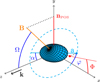 |
Fig. 1 Geometry of a perfectly aligned spinning prolate particle with long-side symmetry axis a. The sky is in the xy plane. The angle Φ (red) is between the x axis and the projection of a onto the plane of the sky. The sightline is the z axis, with electromagnetic wavevector (k) approaching us. The magnetic field (B) lies in the yz plane with the magnetic field angle (Ω) measured from z towards B. The grain spinning plane is perpendicular to B (dashed blue circle) and includes a. The grain spinning angle (φ; blue) is measured on the x axis. The angle of incidence (α) is given between a and k. Note the relation between Ω, α, and φ as given in Eq. (3). |
3.4 Cross-sections per unit mass of dust
The total absorption, scattering, or polarisation cross-section Ki(λ) per unit mass (cm2/g-dust) for dust component i is
 (8)
(8)
where Ci(r, λ) is the corresponding absorption, scattering, or polarisation cross-section for a grain of radius r at wavelength λ (Eqs. (5)-(7)), ρi is the bulk density for population i, and mi is the mass of component i per unit mass of dust:
![Mathematical equation: m_{\rm {i}} = \upmu_{\rm i} \ {\frac{ [\rm{X_{\rm {i}}}]}{[\rm{H}]}} \bigg{/} \sum_{i}{\upmu_{\rm i} \ {\frac{ [\rm{X_{\rm {i}}}]}{[\rm{H}]}}}.](/articles/aa/full_html/2026/05/aa55848-25/aa55848-25-eq14.png) (9)
(9)
The elemental abundance in the dust relative to hydrogen in the gas phase [Xi]/[H] is constrained to respect the depletion limits (Hensley & Draine 2021 ; Siebenmorgen 2023) so that
![Mathematical equation: \frac{[\rm{C}]}{[\rm{Si}]} < 5.2.](/articles/aa/full_html/2026/05/aa55848-25/aa55848-25-eq15.png) (10)
(10)
The total dust cross-section, K(λ), is the sum of Ki from all components1.
3.5 Dust observables in extinction
The optical depth τV = AV/1.086 is
 (11)
(11)
where Nna represents the sum of the dust column density of nanoparticles and amorphous particles, while NμA is the dust column density of micrometre-sized grains. The corresponding mass extinction cross-sections are denoted by  and
and  , respectively. At infinite wavelengths, K(∞) = 0, so AV = −E(∞ - V) > -E(H - V) in the H band. The reddening E(B - V) = 1.086 (τB - τV) is expressed (with our notations) as
 (12)
(12)
providing a second constraint for estimating the relative mass fraction of the micrometre-sized grains, mμA = NμA/(Nn + NμA). From this we derived the absolute reddening of the model,
 (13)
(13)
and the starlight polarisation spectrum,
 (14)
(14)
where N = Nna + NμA (g-dust/cm2) is the total dust column density and Kpol (cm2/g-dust) the total linear polarisation crosssection (Eq. (8)).
The dust model accounts for representative solid-phase element abundances of the main absorbing dust components of the assumed grain stoichiometry and explains phenomena such as wavelength-dependent reddening, starlight polarisation, and the emission of unpolarised and polarised light. It also provides the necessary grey extinction for reconciling the luminosity distances with the Gaia parallaxes (Siebenmorgen et al. 2025). We compared it with the LIPS sample.
3.6 Infrared emission per gram of dust
The emissivity, εi(r), per gram of dust for a grain of population i and particle radius r was determined from the energy balance between emission and absorption of photons from the mean intensity JISRF(λ) of the ISRF (Mathis et al. 1983):
 (15)
(15)
where εi(r) is given by the right-hand side, T refers to the temperature of material i and particle radius r, Bλ(T) is the Planck function, and P(T) is the temperature distribution function (Guhathakurta & Draine 1989; Krügel 2008). This function is evaluated using an iterative scheme by Siebenmorgen et al. (1992). Quantum heating of the dust, and thus P(T), needs to be evaluated only for nanoparticles, as P(T) approaches a δ-function for the larger amorphous and micrometre-sized grains. The total emissivity, e, is the sum of the emissivity from all dust components.
The total polarised emission (εi,pol) of population i was computed by summing the contributions from the minimum alignment radius ( ) to the maximum radius (
 ):
):
 (16)
(16)
where Ki,pol is given by Eq. (8), and T refers to the temperature of material i and particle radius r. The total polarised dust emission, epol, is the sum of the polarised emission from all components contributing to the polarisation, which include the amorphous and the micrometre-sized grains. The corresponding fractional polarisation from dust emission is
 (17)
(17)
3.7 Infrared emission per H atom
More material along a given sightline will increase both E(B - V) and NH. Observationally, it is assumed that the reddening scales approximately linearly with the dust column density and, if well mixed, also with the hydrogen column density such that NH/E(B - V) remains roughly constant. Bohlin et al. (1978) derived NH/E(B - V) = 5.8 (with this value and subsequent values given in 1021 H-atoms cm−2 mag−1), which is close to the value of 5.9 found for translucent clouds (Rachford et al. 2009). However, significantly different values have been reported: 4.9 (Diplas & Savage 1994), 7.5 (Ensor et al. 2017), 9.4 (Nguyen et al. 2018), NHI/E(B - V) = 8.3 (Liszt 2014), and 8.8 (Lenz et al. 2017). These differences are consistent with systematic variations in the gas-to-dust mass ratio, with lower values in the Galactic plane and higher values at high Galactic latitudes.
The total dust mass, Mdust, was estimated by summing all atoms depleted from the gas phase and scaling by the molecular weights corresponding to the assumed grain stoichiometry. The gas mass, Mgas ∼ 1.4 MH, was calculated by summing the contributions of helium and hydrogen, assuming a He:H ratio of 1:10. At high Galactic latitudes, the derived gas-to-dust mass ratio (Mgas/Mdust) is ∼125 (Hensley & Draine 2021; Siebenmorgen 2023). This ratio can vary by up to ∼50% while still being consistent with elemental depletion. However, because we use relative dust abundances in our dust model, such variations, if applied to all components (Eq. (9)), do not affect the fit to the reddening curves.
The gas-to-dust mass ratio and the hydrogen column density are used to scale the dust emission in the model e (Eq. (15)) in erg s−1 Hz−1 sr−1 per g-dust to the Planck surface brightness I (erg s−1 Hz−1 sr−1 cm−2 per H-atom) at 353 GHz, with atomic mass unit mu:
 (18)
(18)
For our nominal dust composition (Sect. 4.1), we find that the NH/E(B - V) ratio is 6.3 for HD 027778, 7.6 for HD 108927, and 7.3 for HD 287150, in units of 1021 H-atoms cm−2 mag−1. These values are consistent with the reference values and fall within the uncertainty range of the gas-to-dust mass ratio (Mgas/Mdust).
3.8 Dust model fitting procedure
The dust model is applied to sightlines with available high-quality far-UV selected reddening curves, visual extinction values derived from Gaia distance estimates (AV; Eq. (21)), near-IR reddening using 2MASS, starlight polarisation spectra obtained with FORS, and the colour-corrected (Planck Collaboration XVII 2014b) total and polarised emission observed by Planck. Best-fit dust parameters are derived using a three-step iterative procedure, under the assumption that along a given sightline where dust extinction dominates, the magnetic-field direction does not vary significantly. For sightlines where the optical polarisation spectrum does not follow the Serkowski curve (Sect. 4.3), the inferred magnetic-field direction should be regarded with caution.
Initially, the reddening curve is fitted using the publicly available χ2 minimisation tool absredgaia (Siebenmorgen 2025). This tool returns the  of the best fit to the reddening curve and the seven model parameters: the exponent of the size distribution (q) and the relative mass fractions of the different dust components: mvgr, mvsi, mpah, maC, maSi, and mμA. These relative dust masses are linked to the element abundances (Eq. (9)). The tool adheres to the depletion limits set by Eq. (10). Dust parameters of the general field of the ISM (Siebenmorgen 2023) are chosen as starting parameters, with an upper radius
  = 3 μm.
In the second step, the starlight polarisation spectrum is fitted by varying the minimum alignment radii of the amorphous carbon and silicate grains,  and
and  , together with the magnetic-field orientation, using Ω = 45° as the initial value. The polarisation spectra of the dust model
  were compared with the FORS data, and the corresponding
  values were computed. The grain radii in the model grid increase by 5% from one bin to the next. The dust model was evaluated for 40 × 40 pairs of
  with i ∈ {aC, aSi} in the range 50-250 nm. The values of
  and
and  that best match the shape of the observed polarisation spectra are identified. Next, the magnetic-field orientation (Ω) was varied and Cpol(Ω, r) (Eq. (5)) computed. The model that best reproduces the Serkowski maximum (pv; Col. 15 of Table 1) was selected. For this value of Ω, a new set of
  and
and  was derived. The best-fitting parameters (
 ,
,  , and Ω) were extracted from the model that minimises
  . Because the extinction cross-section depends on the magnetic-field orientation (Eq. (7)), both steps - fitting the reddening and fitting the polarisation spectra - were iterated.
Planck Collaboration XII (2020) introduced two criteria for constraining dust models by examining the ratio of sub-millimetre-to-optical polarisation. These are the ratio of the fractional polarisation at 850 μm to the optical polarisation efficiency and the ratio of the polarised emission intensity P850 = p850 I850 (MJy/sr) to the optical polarisation,
 (19)
(19)
 (20)
(20)
In the third step, the best-fit parameters from step 2 were retained, and the upper grain radius was varied within the range 0.25 <  ≲ 3 μm. This resulted in 50 models for which the Planck-to-FORS polarisation ratios RS/V and RP/p, along with their corresponding goodness-of-fit parameters
  ,
,  ,
,  , and
, and  , were computed. These χ2 values were normalised to their respective median. We then derived the total goodness-of-fit parameter by assigning equal weight to the reddening curve, the optical polarisation spectrum, and the Planck ratios:
  . The upper radius of the micrometre-sized dust (
 ) corresponds to the minimum of
  . Steps 1-3 were iterated to determine the final set of ten model parameters (Cols. 4-13 in Table 2) for a given axial ratio (a/b) and porosity (VVac) of the grains. The upper grain radius is typically
  = 1 μm, and we identify it with the destruction radius rdes =
  in Eq. (2). Even larger, non-aligned grains could potentially exist, but they would not, or only marginally, contribute to the observations.
The polarised emission spectrum is shown for three sightlines in Fig. 2. At 850 μm, the polarisation is dominated by the micrometre-sized dust particles. By increasing the radius  , these grains become cooler, and their polarisation spectrum shifts to longer wavelengths, so that the polarised intensity P850 increases as long as one remains in the Rayleigh part of the spectrum of the micrometre-sized dust. On the other hand, by decreasing
  , the micrometre-sized agglomerates approach temperatures of the amorphous components, causing the polarisation spectra of the two components to merge.
In the optical range, the micrometre-sized dust provides a grey (constant) reddening and has a marginal impact on the best-fitting model parameters, whereas in the near-IR, the reddening of sightlines with a significant amount of micrometresized grains is strongly impacted by  . Therefore, varying
  will change the fitting parameters of the reddening curve, necessitating repetition of the procedure. Fortunately, in the three steps, the dependences on the free model parameters are weak and converge after one to two iterations. The FORS and Planck data are fitted without considering polarisation by nanoparticles (r < r-pol).
4 Observational constraints on grain structure and alignment efficiency
Observations of dust polarisation in both absorption and emission provide complementary, in principle orthogonal, perspectives on dust grains, allowing constraints to be placed on their shapes, porosity, and alignment efficiencies.
4.1 Pristine sightlines
A high-quality sample of far-UV selected reddening curves was derived by Siebenmorgen et al. (2023). Stars with multiple bright objects in the IUE (Valencic et al. 2004; Fitzpatrick & Massa 2007) and FUSE (Gordon et al. 2009) apertures were excluded. Only stars for which the spectral type and luminosity class, as derived from UVES high-resolution spectroscopy, confirm those used in the reddening estimation were retained. Furthermore, the photometric variability of stars in the high-quality sample, in both the V and G bands, and in the B - V colour, was restricted to ≲0.03 mag.
The visual extinction AV (Table A.1) was derived following Siebenmorgen et al. (2025) by inserting the absolute magnitude MV and Gaia distance estimates DGaia into the photometric equation:
 (21)
(21)
The absolute magnitude (MV) was extracted from the catalogues of Bowen et al. (2008) and Wegner (2006) for the spectral type and luminosity class provided by Siebenmorgen et al. (2023). The distances were estimated using Gaia Data Release 3 (DR3; Gaia Collaboration 2023). To ensure a reliable astrometric solution, only stars with a re-normalised unit weight error below 1.2 were included (Luri et al. 2018). In addition, the G-magnitude-dependent parallax error σ(π, G) was computed following Maíz Apellániz (2022), and only stars with a parallax precision of π/σ(π, G) > 10 were considered. The simple inverse of the DR3 catalogue parallax typically agrees with DGaia within 2%. Since parallactic distances inherently depend on priors, we verified that our distance estimate DGaia aligns with other probabilistic distance estimates within 1-2% (Bailer-Jones et al. 2021).
Three stars exhibiting H-band extinction greater than their visual extinction AV were removed from the subsample, as their luminosity distance is smaller than the trigonometric distance. These selection criteria result in a pristine sample of 27 sightlines that are suitable for dust modelling.
Extinction probes the ISM in the foreground of the star, while emission traces the entire sightline. Planck Collaboration XXI (2015b) established selection criteria for sightlines in order to obtain polarisation measurements of the same dust grains at different wavelengths. For this purpose, the visual extinction derived from the star’s reddening must be comparable to the visual extinction estimated from the Planck maps. This criterion excludes sightlines with significant dust emission originating from material located behind the star. The limited 40′ resolution of the Planck polarisation maps prevents a direct comparison with starlight polarisation measurements of individual stars at low Galactic latitudes. However, at Galactic latitudes |b| ≳ 15°, three stars HD 027778, HD 108927, and HD 287150 exhibit significant starlight and Planck polarisation with comparable extinction values,  (Table A.1). In addition, these stars show the expected reversal in polarisation angle between the polarised emission and the starlight polarisation, consistent with a difference of 90° ± 10°.
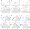 |
Fig. 2 Dust models for HD 027778 (left), HD 108927 (middle), and HD 287150 (right). For each sightline we show, from top to bottom, the reddening curve, the optical polarisation spectrum, and the total and polarised (I and P) dust-emission spectrum. The reddening-curve data with error bars are described in the text. The observed starlight polarisation is shown for the unbinned spectrum (grey lines) and for data binned to a spectral resolution of λ/Δλ ~ 50 (black circles). The dust emission is consistent with Planck 353 GHz measurements (filled circles). Model curves with the adopted a/b ratio and porosity (V) are indicated in the legend. The individual contributions to the observables are shown for nanoparticles (green), amorphous carbon grains (brown), silicates (orange), and micrometre-sized agglomerates (grey shading) for the best-fit model with the parameters listed in Table 2. |
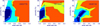 |
Fig. 3 Total goodness-of-fit (χ2tot), normalised to the nominal model (grey symbol), as a function of axial ratio a/b and porosity for HD 027778 (left), HD 108927 (middle), and HD 287150 (right). Regions with successful fits at χ2tot ≲ 1 are shown in blue. |
4.2 Fiducial test cases
The three stars HD 027778, HD 108927, and HD 287150, selected in Sect. 4.1, have optical polarisation spectra and Planck-detected polarised emission measurements of grains from the same environment. They therefore serve as fiducial test cases to investigate the grain structure and alignment. We varied the axial ratio of the prolates for na/b = 5 cases of a/b ∈ {1.5, 2.0, 2.5, 3.0,4.0} and adjusted the porosity, defined as the vacuum volume fraction, of the amorphous carbon and silicate grains for nVa = 7 cases of Va ∈ {0,5,10,20,30,40,50} (%), as well as that of the micrometre-sized dust agglomerates for nVμA = 3 cases of VμA ∈ {5,10,20} (%). We computed the volume ratios of silicate (VSi), carbon (VC), and vacuum (VμA; i.e. porosity) in the fluffy micrometre-sized composites to match an abundance ratio of [Si]/[C] ∼ 3.6 (Hensley & Draine 2021). For the three porosity levels considered for the micrometre-sized dust, their cross-sections were computed using volume ratios VSi:VC:VμA of 57:38:5, 53:37:10, and 48:32:20(%).
We applied the simplified RAT alignment (Eq. (2)) unless stated otherwise. The silicate and dark-dust materials include Fe such that sufficiently large particles are perfectly aligned, falign = 100%. For carbon, the situation is less clear: carbon grains are often assumed to be unaligned, falign = 0, while Herranen et al. (2021) and Andersson et al. (2024) find that grains without magnetic inclusions can reach falign = 50% through RAT alignment. We also experimented with perfect alignment of carbon grains but found that such models fail to reproduce most of the observations. In addition, we examined IDG alignment, noting that this theory neglects internal alignment. The aim is to assess whether IDG can be ruled out when fitting the data. The IDG efficiency parameter δ0 typically varies from one sightline to another between δ0 = 0.2 and 1 μm (Das et al. 2010). The maximum alignment efficiency in IDG is approached asymptotically at δ0 ≳ 10 μm. This corresponds to alignment efficiencies of falign = 18% for δ0 = 0.2 μm, falign = 32% for δ0 = 1 μm, and 46% for δ0 = 10 μm. In total, we inspected nfalign = 5 levels of alignment efficiency. Within this sparsely sampled parameter space of na/b × nVa × nVμA × nfalign = 525 models, we computed the dust cross-sections (Eqs. (7)-(5)) of prolate particles over 300 frequencies, 30 bins of 0° ≲ Ω < 90°, and 130 radii ranging from 6 nm to 3 μm. In these models, a specific set of particle-structure parameters (a/b, Va, VμA) and alignment efficiency (falign) is applied uniformly across all grain types, and the fitting procedure described in Sect. 3.8 is used.
For each star, fits to the reddening curve that respect the elemental depletion constraints (Eq. (10)) and incorporate the Gaia distance estimates (Eq. (21)), together with the FORS starlight polarisation spectrum and the colour-corrected Planck total and polarised dust-emission spectrum, are presented in Fig. 2. The parameter set of the cross-sections with a/b = 2 and Va = VμA = 10% was adopted as the nominal model of the grain structure. In addition, for each star, two alternative models are shown that achieve a fit of comparable quality to the nominal model.
For HD 027778 and HD 108927, the best fits are obtained when neglecting the alignment of carbon grains, although for HD 027778 a comparably good fit is also achieved when assuming falign(aC) = 50%. In contrast, for HD 287150, aligned carbon grains make an important contribution to the optical polarisation and dominate the polarised emission. Models that ignore the alignment of aC grains for HD 287150 show a too-steep decline in the polarisation at λ > 0.7 μm to reproduce the optical polarisation spectrum, and they underpredict P850 by a factor of two. This underprediction of the polarisation in the optical and submillimetre can be compensated by a substantial increase in the mass of the micrometre-sized grains, which, however, leads to an overprediction of the near-IR reddening towards HD 287150.
In the optical, the polarisation cross-section Kpol can be dominated by aC grains if aligned, and otherwise by aSi grains. In this wavelength range, μA grains, if present, contribute only weakly, whereas they dominate Kpol at λ > 1 μm. Because aSi and μA grains attain similar temperatures, the polarised emission in Fig. 2 is dominated by the micrometre-sized agglomerates when aC grains are not aligned. Notably, the optical and sub-millimetre polarisation arise from distinct grain populations. Following Fanciullo et al. (2015), we estimated the intensity scaling parameter (G0) of the ISRF from Planck (Planck Collaboration XI 2014a) and IRAS observations, and the visual extinction AV (Table A.1) to the stars. We find G0 = 0.56, 0.37, and 0.43 for HD 027778, HD 108927, and HD 287150. No trend is found between aC alignment and G0.
There are degeneracies in the model grid of particle structures, where multiple models match all datasets with similarly good quality. In Fig. 3, the total goodness of fit, χ2ot, normalised to the nominal model, is shown as a function of axial ratio and porosity. The contour levels at  highlight regions of comparable fit quality; these are marked in blue and correspond to models performing similarly to the nominal model (Fig. 3). Such models typically exhibit grain porosities Va ≲ 20 % and axial ratios a/b ≲ 2.5. The nominal model yields the lowest
  across the three stars for which both FORS spectra of the dichroic polarisation and Planck polarised-emission data are available. For these models, the upper radius of the grains, as derived from the Planck polarisation (Eqs. (19) and (20)), is
  = 1 μm; the other model parameters are listed in Table 2.
Dust parameters of the 27 sightlines that have been modelled.
4.3 Dust modelling of individual sightlines
The dust model is applied to the remaining 24 sightlines selected in Sect. 4.1, for which polarised emission data from the same grains responsible for the optical polarisation are not available. These stars are located at |b| < 15°, where the Planck observations suffer from low (40′) spatial resolution. The expected 90° flip in the polarisation angle between dichroic polarisation and polarised emission is also not observed (Table A.1).
The reddening curves and starlight polarisation spectra are fitted using Steps 1 and 2 of the fitting procedure (Sect. 3.8). The grain structures of the nominal model (a/b = 2, V = 10%), together with the three other combinations of a/b ∈ {1.5,2} and V ∈ {5,10}(%), are used. We adopted as default RAT alignment with perfectly aligned silicates, falign = 100%, and include or exclude alignment of carbon grains with falign(aC) ∈ {0,50}%, as well as alignment of micrometre-sized dust with falign = 100%. For comparison, IDG alignment is also applied using a size dependence similar to Eq. (2) (Siebenmorgen et al. 2014). The model fits and the contributions of the different grain components to the absolute reddening and the optical polarisation spectra are shown in Figs. 4 and 5, respectively.
The dust parameters and three derived quantities are listed for all 27 sightlines in Table 2. The axial ratios and porosities are given in Cols. 2 and 3. The model with a/b = 2 and a porosity of 10% is preferred for 11 sightlines (63%), while the model with a/b = 1.5 and a porosity of 5% provides a slightly lower  for 16 sightlines. Except for two cases, the maximum grain radius is
  .
.
The relative masses mvgr, mvSi, mPAH, maC, maSi, and mμA in 1 g of dust (%) for the individual dust components are listed in Table 2, Cols. 4-9. The percentage contribution of the micrometre-sized grains to the total extinction in the optical is given in Col. 16. Typically, about one-third of the dust mass resides in micrometre-sized dust agglomerates, which also contribute about one-third of the total extinction AV (Table 2).
The exponent of the dust size distribution q, the minimum alignment radii of amorphous silicate and carbon grains, r-pol,Si and r-pol,aC, and the derived magnetic field orientation Ω are given in Table 2, Cols. 10-13. Additional derived quantities include the total Si and C abundances in dust relative to H (in ppm; Cols. 14-15). The typical abundances, [Si]/[H] ∼ 37 ppm and [C]/[H] ∼ 96 ppm, agree with estimates for the diffuse ISM by Hensley & Draine (2021). The median values and the 1σ scatter of the parameters are provided at the bottom of the table. The large scatter indicates substantial variation across individual sightlines.
As shown in Fig. 4, sightlines containing a significant amount of dark dust are dominated in the near-IR reddening by these micrometre-sized grains, which produce grey (constant) extinction in the optical. The amorphous grains produce a linear rise in extinction in the optical and add grey extinction in the far-UV. Nanoparticles are responsible for the 2175 Å extinction bump and the steep far-UV rise.
The polarisation spectra (Fig. 5) generally follow the Serkowski law with λmax in the visible. Seven stars peak in the B band, and twelve stars peak at λmax > 0.65 μm (Table A.1). The Serkowski fit is usually interpreted as tracing the characteristic size of aligned grains in a single absorbing cloud, although this is a simplification (Andersson et al. 2011). The polarisation results from the sum of contributions from silicate grains, dark dust, and (when aligned) amorphous carbon particles. These components peak at different wavelengths, and this could be caused by different clouds being located along the sightline (Mandarakas et al. 2025).
A noticeable deviation from the Serkowski curve is seen towards HD 093222, where the polarisation peaks at λmax = 0.43 μm and, after an initial decline, rises again at 0.7 μm towards the IR (Fig. 5). A strong wavelength gradient in the polarisation angle, dθ/dλ = 97°/μm, is also observed (Table A.1).
In a single-cloud scenario with a common magnetic field, the polarisation angle should remain constant and the polarisation should peak for typical ISM grain sizes at λmax = 0.55 μm. Indeed, Mandarakas et al. (2025) reproduce the observed wavelength dependence of the polarisation angle towards HD 093222 using a two-cloud model. Two additional multiple-cloud sightlines in our sample, HD 037903 and HD 152245, show variations in polarisation angle, with dθ/dλ = 5.3 and 6.8°/μm and maxima at λmax = 0.66 and 0.62 μm, respectively. Five single-cloud sightlines2 show variations of 6.6 ≲ dθ/dλ ≲ 18.5 (°/μm), while the remaining sightlines exhibit a weak wavelength dependence with dθ/dλ < 5°/μm (Table A.1, Fig. A.2).
The model fits the optical polarisation spectra typically within 1σ of the FORS data rebinned to λ/Δλ ~ 50 (Fig. 5). The contributions of the individual grain components to the optical polarisation spectra are shown in Fig. 5. Most of the polarisation, especially in the V band and at shorter wavelengths, is produced by silicate grains with a minimum alignment radius of  = 118 ± 23 nm. For half of the sightlines, the polarisation spectra are better reproduced when aligned carbon particles are included, with
  = 69 ± 25 nm. The contribution from micrometre-sized grains rises steadily from p ~ 0.1% in the UV to p ≲ 0.5% at 0.9 μm. These grains dominate the polarised emission in the (sub-)millimetre regime (Fig. 2).
The IDG model predicts lower alignment efficiency than RAT. Fits to the optical polarisation spectra using IDG systematically require the maximal alignment efficiency allowed by this model, with both silicate and carbon grains being aligned. Note that the lower alignment efficiencies in IDG are compensated in the fits (orange lines in Fig. 5) by increasing the axial ratio to typically a/b = 2.5, the porosity to 10%, and by overestimating the magnetic-field orientation Ω, typically by a factor of two.
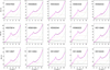 |
Fig. 4 Dust model fits to the absolute reddening curves, E(λ - V), of 24 sightlines. Data (circles) cover 0.09-2.2 μm and are complemented at infinite wavelengths by -AV (Table A.1). The best fit, with contributions from nanoparticles (green), amorphous silicates and carbon grains (brown), and micrometre-sized dust agglomerates (dark), is shown, with the model parameters listed in Table 2. Notably, the micrometre-sized grains dominate in the IR and provide a wavelength-independent contribution in the optical and far-UV. |
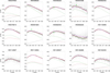 |
Fig. 5 Dust model fits to optical polarisation spectra obtained with FORS for 24 sightlines. Observations are shown as the original unbinned spectrum (grey lines) and re-binned to a spectral resolution of λ/Δλ ~ 50 (black open circles). The error bars associated with the re-binned spectra correspond to 1 σ. In each panel, best-fit dust models that adopt maximum IDG alignment efficiency are shown in ochre, while models based on RAT alignment are shown by the magenta line, with individual contributions from amorphous silicates (green line), carbon grains (brown line), and micrometre-sized dust agglomerates (black line) also indicated. Data available in the stellar polarisation catalogue by Heiles (2000) are shown with a green circle. |
5 Conclusion
We have completed the LIPS, which obtained FORS spec-tropolarimetry in the 0.38-0.92 μm wavelength range for 161 sightlines through the diffuse ISM. Sixty polarisation spectra are presented in this work. The LIPS sample was selected based on the availability of reddening curves: in the far-UV from the IUE and FUSE satellite missions, in the optical from ground-based photometry, and in the near-IR from 2MASS. High-resolution spectra were obtained with UVES/VLT to verify the spectral types and luminosity classes of the stars used for deriving the reddening curves and to probe the number of clouds along individual sightlines. Gaia parallaxes were used to estimate the visual extinction (AV) necessary for reconciling the derived luminosity distances with the trigonometric distance estimates for the same stars. The starlight polarisation spectra were complemented by Planck 850 μm polarimetry.
This dataset was used to constrain the properties of grains in the diffuse ISM using a three-component model from Siebenmorgen (2023) that includes nanoparticles, amorphous grains, and micrometre-sized grains. The nanoparticles are responsible for the far-UV rise in the reddening curve, the 2175 Å bump, and the mid-IR emission bands. The amorphous grains produce grey (constant) extinction in the far-UV, an almost linear decline towards longer wavelengths, and the far-IR emission. The micrometre-sized particles contribute grey extinction in the optical, a linear decline in the near-IR, and the submillimetre emission. The optical polarisation is dominated by amorphous grains, while the 850 μm polarisation is dominated by the micrometre-sized dust agglomerates unless amorphous carbon particles are also aligned.
Within the sample, three sightlines exhibit both significant starlight and Planck polarisation, with comparable extinction values,  ∼ AV, and the expected 90° reversal in the polarisation angle between polarised emission and starlight polarisation. The polarisation data for these sightlines provide an almost orthogonal perspective on the aligned grains, enabling constraints to be placed on their particle shape, porosity, and alignment efficiency. Although degeneracies exist among the dust model parameters, a good fit to all data for these three sightlines is obtained using an axial ratio a/b = 2 and porosities of 10% for both the amorphous and micrometre-sized grains.
We applied RAT (Hoang & Lazarian 2016) in the simplified formulation from Reissl et al. (2020), assuming perfect alignment for silicate and micrometre-sized dust. For carbon grains, we considered two cases, either including alignment with falign(aC) = 50% or assuming no alignment. This nominal model was applied to 24 additional sightlines for which high-quality reddening curves and optical polarisation spectra were available but for which the Planck polarisation data were ambiguous. For half of these sightlines, the best fits include aligned carbon grains. A single-cloud model generally provides fits consistent within the 1σ uncertainties. The IDG models, which ignore internal alignment, reproduce the optical polarisation only when forced to their asymptotic maximum alignment for both silicate and carbon grains, at the cost of overestimating parameters such as the magnetic field orientation (Ω).
The contribution of micrometre-sized dust is most evident in the near-IR extinction and, with few exceptions, is marginal in the optical spectropolarimetry. Overall, we find that micrometresized dust is responsible for approximately one-third of the total extinction and comprises one-third of the total dust mass. Significant variations in dust abundances persist from cloud to cloud.
The present analysis is limited by the low spatial resolution of the Planck maps, which leads to source confusion. A follow-up sub-millimetre survey with a high-spatial-resolution polarimeter is required, once it becomes available, to combine polarised emission and starlight polarisation measurements through the diffuse ISM.
Data availability
The Fortran code of the dust model described in Siebenmorgen & Heymann (2026a) and the corresponding library of dust cross-sections for spheroidal grains (Siebenmorgen & Heymann 2026b) are publicly available. The processed FORS polarisation spectra presented in this work are available at the CDS via https://cdsarc.cds.unistra.fr/viz-bin/cat/J/A+A/709/A277
Acknowledgements
We thank the referee for the valuable and constructive comments, in particular regarding the consideration of radiative torque alignment (RAT) theory. This research has made use of the services of the ESO Science Archive Facility and of the SIMBAD database, operated at the CDS, Strasbourg, France. This work is partially based on observations collected at the European Southern Observatory under ESO programme 102.C-0040.
References
- Allamandola, L. J., Tielens, A. G. G. M., & Barker, J. R. 1989, ApJS, 71, 7331 [Google Scholar]
- Andersson, B.-G., Pintado, O., Potter, S. B., Straižys, V., & Charcos-Llorens, M. 2011, A&A, 534, A19 [NASA ADS] [CrossRef] [EDP Sciences] [Google Scholar]
- Andersson, B.-G., Lazarian, A., & Vaillancourt, J. E. 2015, ARA&A, 53, 501 [Google Scholar]
- Andersson, B.-G., Karoly, J., Bastien, P., et al. 2024, ApJ, 963, 76 [NASA ADS] [CrossRef] [Google Scholar]
- Appenzeller, I., Fricke, K., Fürtig, W., et al. 1998, The Messenger, 94, 11 [Google Scholar]
- Bagnulo, S., Cox, N. L. J., Cikota, A., et al. 2017, A&A, 608, A1461 [Google Scholar]
- Bailer-Jones, C. A. L., Rybizki, J., Fouesneau, M., Demleitner, M., & Andrae, R. 2021, AJ, 161, 147 [Google Scholar]
- Bianchi, S. 2024, A&A, 691, A330 [NASA ADS] [CrossRef] [EDP Sciences] [Google Scholar]
- Blasberger, A., Behar, E., Perets, H. B., Brosch, N., & Tielens, A. G. G. M. 2017, ApJ, 836, 173 [NASA ADS] [CrossRef] [Google Scholar]
- Bohlin, R. C., Savage, B. D., & Drake, J. F. 1978, ApJ, 224, 132 [Google Scholar]
- Bohren, C. F., & Huffman, D. R. 1983, Absorption and Scattering of Light by Small Particles, Research supported by the University of Arizona and Institute of Occupational and Environmental Health (New York, Wiley-Interscience), 1983, 541 [Google Scholar]
- Bowen, D. V., Jenkins, E. B., Tripp, T. M., et al. 2008, ApJS, 176, 59 [NASA ADS] [CrossRef] [Google Scholar]
- Chini, R., Krügel, E., Haslam, C. G. T., et al. 1993, A&A, 272, L5 [NASA ADS] [Google Scholar]
- Chini, R., Krügel, E., Lemke, R., & Ward-Thompson, D. 1995, A&A, 295, 317 [NASA ADS] [Google Scholar]
- Cutri, R. M., Skrutskie, M. F., van Dyk, S., et al. 2003, 2MASS All Sky Catalog of point sources. (ADS) [Google Scholar]
- Das, H. K., Voshchinnikov, N. V., & Il’in, V. B. 2010, MNRAS, 404, 265 [NASA ADS] [Google Scholar]
- Davis, Jr., L., & Greenstein, J. L. 1951, ApJ, 114, 206 [NASA ADS] [CrossRef] [Google Scholar]
- Dekker, H., D’Odorico, S., Kaufer, A., Delabre, B., & Kotzlowski, H. 2000, SPIE Conf. Ser., 4008, 534 [Google Scholar]
- Demyk, K., Gromov, V., Meny, C., et al. 2022, A&A, 666, A192 [NASA ADS] [CrossRef] [EDP Sciences] [Google Scholar]
- Diplas, A., & Savage, B. D. 1994, ApJ, 427, 274 [Google Scholar]
- Dolginov, A. Z., & Mitrofanov, I. G. 1976, Ap&SS, 43, 291 [NASA ADS] [CrossRef] [Google Scholar]
- Dorschner, J., Begemann, B., Henning, T., Jaeger, C., & Mutschke, H. 1995, A&A, 300, 503 [Google Scholar]
- Draine, B. T. 2003, ApJ, 598, 1017 [NASA ADS] [CrossRef] [Google Scholar]
- Draine, B. T., & Fraisse, A. A. 2009, ApJ, 696, 1 [Google Scholar]
- Draine, B. T., & Hensley, B. S. 2021, ApJ, 909, 94 [NASA ADS] [CrossRef] [Google Scholar]
- Draine, B. T., & Weingartner, J. C. 1996, ApJ, 470, 551 [NASA ADS] [CrossRef] [Google Scholar]
- Ensor, T., Cami, J., Bhatt, N. H., & Soddu, A. 2017, ApJ, 836, 162 [Google Scholar]
- Fanciullo, L., Guillet, V., Aniano, G., et al. 2015, A&A, 580, A136 [NASA ADS] [CrossRef] [EDP Sciences] [Google Scholar]
- Fitzpatrick, E. L., & Massa, D. 2007, ApJ, 663, 320 [Google Scholar]
- Gaia Collaboration (Vallenari, A., et al.) 2023, A&A, 674, A1 [NASA ADS] [CrossRef] [EDP Sciences] [Google Scholar]
- Galametz, M., Madden, S., Galliano, F., et al. 2009, A&A, 508, 645 [NASA ADS] [CrossRef] [EDP Sciences] [Google Scholar]
- Galliano, F., Madden, S. C., Jones, A. P., Wilson, C. D., & Bernard, J. P. 2005, A&A, 434, 867 [CrossRef] [EDP Sciences] [Google Scholar]
- Giang, N. C., Le Gouellec, V. J. M., Hoang, T., Maury, A. J., & Hennebelle, P. 2025, ApJ, 980, 105 [Google Scholar]
- Gordon, K. D., Cartledge, S., & Clayton, G. C. 2009, ApJ, 705, 1320 [NASA ADS] [CrossRef] [Google Scholar]
- Guhathakurta, P., & Draine, B. T. 1989, ApJ, 345, 230 [NASA ADS] [CrossRef] [Google Scholar]
- Guillet, V., Fanciullo, L., Verstraete, L., et al. 2018, A&A, 610, A16 [NASA ADS] [CrossRef] [EDP Sciences] [Google Scholar]
- Hall, J. S. 1949, Science, 109, 166 [NASA ADS] [CrossRef] [Google Scholar]
- Heiles, C. 2000, AJ, 119, 923 [Google Scholar]
- Hensley, B. S., & Draine, B. T. 2021, ApJ, 906, 73 [NASA ADS] [CrossRef] [Google Scholar]
- Herranen, J., Lazarian, A., & Hoang, T. 2021, ApJ, 913, 63 [NASA ADS] [CrossRef] [Google Scholar]
- Hildebrand, R. H. 1988, QJRAS, 29, 327 [NASA ADS] [Google Scholar]
- Hiltner, W. A. 1949, Science, 109, 165 [NASA ADS] [CrossRef] [Google Scholar]
- Hoang, T., & Lazarian, A. 2016, ApJ, 831, 159 [Google Scholar]
- Hoang, T., & Truong, B. 2024, ApJ, 965, 183 [NASA ADS] [CrossRef] [Google Scholar]
- Hoang, T., Tram, L. N., Lee, H., Diep, P. N., & Ngoc, N. B. 2021, ApJ, 908, 218 [NASA ADS] [CrossRef] [Google Scholar]
- Hong, S. S., & Greenberg, J. M. 1980, A&A, 88, 194 [NASA ADS] [Google Scholar]
- Jones, R. V., & Spitzer, Jr., L. 1967, ApJ, 147, 943 [NASA ADS] [CrossRef] [Google Scholar]
- Kennicutt, R. C., Calzetti, D., Aniano, G., et al. 2011, PASP, 123, 1347 [Google Scholar]
- Kim, S.-H., & Martin, P. G. 1995, ApJ, 444, 293 [Google Scholar]
- Krügel, E. 2008, An Introduction to the Physics of Interstellar Dust (UK: IOP) [Google Scholar]
- Krügel, E., & Siebenmorgen, R. 1994, A&A, 288, 929 [Google Scholar]
- Krügel, E., Siebenmorgen, R., Zota, V., & Chini, R. 1998, A&A, 331, L91 [Google Scholar]
- Krüger, H., Strub, P., Grün, E., & Sterken, V. J. 2015, ApJ, 812, 139 [CrossRef] [Google Scholar]
- Landgraf, M., Baggaley, W. J., Grün, E., Krüger, H., & Linkert, G. 2000, J. Geophys. Res., 105, 10343 [NASA ADS] [CrossRef] [Google Scholar]
- Lazarian, A. 1997, MNRAS, 288, 609 [Google Scholar]
- Lazarian, A., & Hoang, T. 2007, MNRAS, 378, 910 [Google Scholar]
- Lenz, D., Hensley, B. S., & Doré, O. 2017, ApJ, 846, 38 [NASA ADS] [CrossRef] [Google Scholar]
- Liszt, H. 2014, ApJ, 780, 10 [Google Scholar]
- Luri, X., Brown, A. G. A., Sarro, L. M., et al. 2018, A&A, 616, A9 [NASA ADS] [CrossRef] [EDP Sciences] [Google Scholar]
- Madden, S. C., Rémy-Ruyer, A., Galametz, M., et al. 2013, PASP, 125, 600 [NASA ADS] [CrossRef] [Google Scholar]
- Maíz Apellániz, J. 2022, A&A, 657, A130 [NASA ADS] [CrossRef] [EDP Sciences] [Google Scholar]
- Mandarakas, N., Tassis, K., & Skalidis, R. 2025, A&A, 698, A168 [NASA ADS] [CrossRef] [EDP Sciences] [Google Scholar]
- Mathis, J. S., Mezger, P. G., & Panagia, N. 1983, A&A, 128, 212 [NASA ADS] [Google Scholar]
- Mathis, J. S., Rumpl, W., & Nordsieck, K. H. 1977, ApJ, 217, 425 [Google Scholar]
- Nguyen, H., Dawson, J. R., Miville-Deschênes, M. A., et al. 2018, ApJ, 862, 49 [NASA ADS] [CrossRef] [Google Scholar]
- Ormel, C. W., Min, M., Tielens, A. G. G. M., Dominik, C., & Paszun, D. 2011, A&A, 532, A43 [NASA ADS] [CrossRef] [EDP Sciences] [Google Scholar]
- Planck Collaboration XI. 2014a, A&A, 571, A11 [NASA ADS] [CrossRef] [EDP Sciences] [Google Scholar]
- Planck Collaboration XVII. 2014b, A&A, 566, A55 [NASA ADS] [CrossRef] [EDP Sciences] [Google Scholar]
- Planck Collaboration XIX. 2015a, A&A, 576, A104 [NASA ADS] [CrossRef] [EDP Sciences] [Google Scholar]
- Planck Collaboration XXI. 2015b, A&A, 576, A106 [NASA ADS] [CrossRef] [EDP Sciences] [Google Scholar]
- Planck Collaboration XII. 2020, A&A, 641, A12 [NASA ADS] [CrossRef] [EDP Sciences] [Google Scholar]
- Popovic, B., Wiseman, P., Sullivan, M., et al. 2024, MNRAS, 534, 2263 [Google Scholar]
- Puget, J. L., & Leger, A. 1989, ARA&A, 27, 161 [Google Scholar]
- Purcell, E. M. 1979, ApJ, 231, 404 [NASA ADS] [CrossRef] [Google Scholar]
- Rachford, B. L., Snow, T. P., Destree, J. D., et al. 2009, ApJS, 180, 125 [NASA ADS] [CrossRef] [Google Scholar]
- Reissl, S., Guillet, V., Brauer, R., et al. 2020, A&A, 640, A118 [NASA ADS] [CrossRef] [EDP Sciences] [Google Scholar]
- Rémy-Ruyer, A., Madden, S. C., Galliano, F., et al. 2013, A&A, 557, A95 [Google Scholar]
- Roberge, W. G., & Lazarian, A. 1999, MNRAS, 305, 615 [NASA ADS] [CrossRef] [Google Scholar]
- Serkowski, K., Mathewson, D. S., & Ford, V. L. 1975, ApJ, 196, 261 [NASA ADS] [CrossRef] [Google Scholar]
- Siebenmorgen, R. 2023, A&A, 670, A115 [NASA ADS] [CrossRef] [EDP Sciences] [Google Scholar]
- Siebenmorgen, R. 2025, https://doi.org/10.5281/zenodo.14624100 [Google Scholar]
- Siebenmorgen, R., & Heymann, F. 2026a, https://doi.org/10.5281/zenodo.19190239 [Google Scholar]
- Siebenmorgen, R., & Heymann, F. 2026b, https://doi.org/10.5281/zenodo.19236224 [Google Scholar]
- Siebenmorgen, R., Heymann, F., & Chini, R. 2025, ApJ, 979, L45 [Google Scholar]
- Siebenmorgen, R., Kruegel, E., & Mathis, J. S. 1992, A&A, 266, 501 [Google Scholar]
- Siebenmorgen, R., Krügel, E., & Chini, R. 1999, A&A, 351, 495 [NASA ADS] [Google Scholar]
- Siebenmorgen, R., Voshchinnikov, N. V., & Bagnulo, S. 2014, A&A, 561, A82 [NASA ADS] [CrossRef] [EDP Sciences] [Google Scholar]
- Siebenmorgen, R., Voshchinnikov, N. V., Bagnulo, S., et al. 2018, A&A, 611, A5 [NASA ADS] [CrossRef] [EDP Sciences] [Google Scholar]
- Siebenmorgen, R., Krelowski, J., Smoker, J., Galazutdinov, G., & Bagnulo, S. 2020, A&A, 641, A35 [NASA ADS] [CrossRef] [EDP Sciences] [Google Scholar]
- Siebenmorgen, R., Smoker, J., Krelowski, J., Gordon, K., & Chini, R. 2023, A&A, 676, A132 [NASA ADS] [CrossRef] [EDP Sciences] [Google Scholar]
- Smoker, J., Haddad, N., Iwert, O., et al. 2009, The Messenger, 138, 8 [NASA ADS] [Google Scholar]
- Stecher, T. P., & Donn, B. 1965, ApJ, 142, 1681 [NASA ADS] [CrossRef] [Google Scholar]
- Vaillancourt, J. E., Andersson, B. G., Clemens, D. P., et al. 2020, ApJ, 905, 157 [NASA ADS] [CrossRef] [Google Scholar]
- Valencic, L. A., Clayton, G. C., & Gordon, K. D. 2004, ApJ, 616, 912 [NASA ADS] [CrossRef] [Google Scholar]
- Voshchinnikov, N. V. 2004, Astrophys. Space Phys. Res., 12, 1 [NASA ADS] [Google Scholar]
- Voshchinnikov, N. V. 2012, J. Quant. Spec. Radiat. Transf., 113, 2334 [NASA ADS] [CrossRef] [Google Scholar]
- Voshchinnikov, N. V., & Farafonov, V. G. 1993, Ap&SS, 204, 19 [NASA ADS] [CrossRef] [Google Scholar]
- Wang, S., Li, A., & Jiang, B. W. 2015a, MNRAS, 454, 569 [NASA ADS] [CrossRef] [Google Scholar]
- Wang, S., Li, A., & Jiang, B. W. 2015b, ApJ, 811, 38 [NASA ADS] [CrossRef] [Google Scholar]
- Wegner, W. 2006, MNRAS, 371, 185 [NASA ADS] [CrossRef] [Google Scholar]
- Westphal, A. J., Stroud, R. M., Bechtel, H. A., et al. 2014, Science, 345, 786 [Google Scholar]
- Ysard, N., Jones, A. P., Guillet, V., et al. 2024, A&A, 684, A34 [NASA ADS] [CrossRef] [EDP Sciences] [Google Scholar]
- Zubko, V. G., Mennella, V., Colangeli, L., & Bussoletti, E. 1996, MNRAS, 282, 1321 [Google Scholar]
A suffix or index ‘abs’ indicates absorption, ‘ext’ extinction, ‘pol’ polarisation, ‘sca’ scattering, ‘des’ destruction, ‘tot’ total, and ‘μA’ micrometre-sized agglomerates.
HD 054439, HD 046223, HD 092044, HD 038023, and HD 294304.
Appendix A Tables and figures
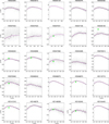 |
Fig. A.1 FORS polarisation spectra of 43 stars. The grey lines show the original data, and the black open circles (with 1 σ error bars) represent the data re-binned to a spectral resolution of λ/Δλ ~ 50. The green circles represent the measurements available in the catalogue by Heiles (2000). The magenta lines show the best fits obtained with the Serkowski formula. |
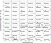 |
Fig. A.2 Position angle of the polarisation for the 60 stars in the LIPS sample analysed in this work, offset with respect to its value in the V optical filter, θ - θV (see Table A.1). Data available in the catalogue by Heiles (2000) are shown with green circles. |
Stars with derived Planck, reddening, FORS, and Serkowski fit parameters.
All Tables
All Figures
|
Fig. 1 Geometry of a perfectly aligned spinning prolate particle with long-side symmetry axis a. The sky is in the xy plane. The angle Φ (red) is between the x axis and the projection of a onto the plane of the sky. The sightline is the z axis, with electromagnetic wavevector (k) approaching us. The magnetic field (B) lies in the yz plane with the magnetic field angle (Ω) measured from z towards B. The grain spinning plane is perpendicular to B (dashed blue circle) and includes a. The grain spinning angle (φ; blue) is measured on the x axis. The angle of incidence (α) is given between a and k. Note the relation between Ω, α, and φ as given in Eq. (3). |
| In the text | |
|
Fig. 2 Dust models for HD 027778 (left), HD 108927 (middle), and HD 287150 (right). For each sightline we show, from top to bottom, the reddening curve, the optical polarisation spectrum, and the total and polarised (I and P) dust-emission spectrum. The reddening-curve data with error bars are described in the text. The observed starlight polarisation is shown for the unbinned spectrum (grey lines) and for data binned to a spectral resolution of λ/Δλ ~ 50 (black circles). The dust emission is consistent with Planck 353 GHz measurements (filled circles). Model curves with the adopted a/b ratio and porosity (V) are indicated in the legend. The individual contributions to the observables are shown for nanoparticles (green), amorphous carbon grains (brown), silicates (orange), and micrometre-sized agglomerates (grey shading) for the best-fit model with the parameters listed in Table 2. |
| In the text | |
|
Fig. 3 Total goodness-of-fit (χ2tot), normalised to the nominal model (grey symbol), as a function of axial ratio a/b and porosity for HD 027778 (left), HD 108927 (middle), and HD 287150 (right). Regions with successful fits at χ2tot ≲ 1 are shown in blue. |
| In the text | |
|
Fig. 4 Dust model fits to the absolute reddening curves, E(λ - V), of 24 sightlines. Data (circles) cover 0.09-2.2 μm and are complemented at infinite wavelengths by -AV (Table A.1). The best fit, with contributions from nanoparticles (green), amorphous silicates and carbon grains (brown), and micrometre-sized dust agglomerates (dark), is shown, with the model parameters listed in Table 2. Notably, the micrometre-sized grains dominate in the IR and provide a wavelength-independent contribution in the optical and far-UV. |
| In the text | |
|
Fig. 5 Dust model fits to optical polarisation spectra obtained with FORS for 24 sightlines. Observations are shown as the original unbinned spectrum (grey lines) and re-binned to a spectral resolution of λ/Δλ ~ 50 (black open circles). The error bars associated with the re-binned spectra correspond to 1 σ. In each panel, best-fit dust models that adopt maximum IDG alignment efficiency are shown in ochre, while models based on RAT alignment are shown by the magenta line, with individual contributions from amorphous silicates (green line), carbon grains (brown line), and micrometre-sized dust agglomerates (black line) also indicated. Data available in the stellar polarisation catalogue by Heiles (2000) are shown with a green circle. |
| In the text | |
|
Fig. A.1 FORS polarisation spectra of 43 stars. The grey lines show the original data, and the black open circles (with 1 σ error bars) represent the data re-binned to a spectral resolution of λ/Δλ ~ 50. The green circles represent the measurements available in the catalogue by Heiles (2000). The magenta lines show the best fits obtained with the Serkowski formula. |
| In the text | |
|
Fig. A.2 Position angle of the polarisation for the 60 stars in the LIPS sample analysed in this work, offset with respect to its value in the V optical filter, θ - θV (see Table A.1). Data available in the catalogue by Heiles (2000) are shown with green circles. |
| In the text | |
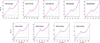 |
Fig. A.3 Dust model fits to the absolute reddening curves, continued from Fig. 4. |
| In the text | |
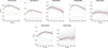 |
Fig. A.4 FORS polarisation spectra and models, continued from Fig. 5. |
| In the text | |
Current usage metrics show cumulative count of Article Views (full-text article views including HTML views, PDF and ePub downloads, according to the available data) and Abstracts Views on Vision4Press platform.
Data correspond to usage on the plateform after 2015. The current usage metrics is available 48-96 hours after online publication and is updated daily on week days.
Initial download of the metrics may take a while.