| Issue |
A&A
Volume 709, May 2026
|
|
|---|---|---|
| Article Number | A266 | |
| Number of page(s) | 19 | |
| Section | Interstellar and circumstellar matter | |
| DOI | https://doi.org/10.1051/0004-6361/202555630 | |
| Published online | 22 May 2026 | |
Preferential accretion of binary stars
Niels Bohr Institute, University of Copenhagen,
Jagtvej 155 A,
2200
Copenhagen,
Denmark
★ Corresponding authors: This email address is being protected from spambots. You need JavaScript enabled to view it.
; This email address is being protected from spambots. You need JavaScript enabled to view it.
; This email address is being protected from spambots. You need JavaScript enabled to view it.
Received:
22
May
2025
Accepted:
2
October
2025
Abstract
The attractive properties of gravity enable matter in dense cores to collapse into stars, spanning seven orders of magnitude in space and time, which makes modelling star formation a challenging multi-scale process. To circumvent this scale problem, stars are replaced by a sub-grid sink particle at a much larger scale. Sink particles are created above a threshold density and acquire mass and momentum through accretion. In models where binary star systems form and migrate to separations of a few cells, the accretion flow is unresolved and the relative accretion rate to the sink particles may become inaccurate. We introduce a new recipe for accretion onto binary sink particles that have overlapping accretion regions, and we implement an algorithm to track the angular momentum of sink particles as a proxy for stellar spin. Our preferential binary accretion recipe uses a virtual binary sink particle for the purpose of accretion and redistributes the accreted mass onto the sink particles according to results from models investigating binary accretion in detail. This solves problems common to current algorithms in many codes: (i) accretion is not suppressed due to large velocity differences between gas and stars, when that velocity is only internal to the binary system; (ii) the accretion rates are smoother for the unresolved close binaries in eccentric orbits; and (iii) non-physical suppression of accretion onto the secondary sink particle, when the primary dominates the potential, is eliminated. We test our implementation by comparing simulations at increasing resolution until the binaries are resolved. While not perfect, the algorithm mitigates undesired properties of current algorithms and is particularly useful for global models of star-forming regions. It may also be applied to other unresolved accreting binaries, such as compact objects in evolved star clusters and binary supermassive black holes in cosmological models.
Key words: accretion, accretion disks / methods: numerical / binaries: general / stars: formation / stars: pre-main sequence / stars: protostars
© The Authors 2026
 Open Access article, published by EDP Sciences, under the terms of the Creative Commons Attribution License (https://creativecommons.org/licenses/by/4.0), which permits unrestricted use, distribution, and reproduction in any medium, provided the original work is properly cited.
This article is published in open access under the Subscribe to Open model. This email address is being protected from spambots. You need JavaScript enabled to view it. to support open access publication.
1 Introduction
The always-attracting property of gravity causes matter in dense cores, extending up to around 10 000 AU, to collapse into stars that are only 0.001 AU in size. The cores are not isolated, and during the formation process, turbulent and filamentary streamers originating up to millions of AU away fuel the process (Pineda et al. 2023). This makes star formation a multi-scale, multi-physics problem requiring modelling over more than seven orders of magnitude in space and time. Recent codes with sophisticated algorithms, such as adaptive mesh refinement, can span such a dynamic range (Kuffmeier et al. 2018) and follow the collapse of matter in a single, isolated core to stellar densities for short time spans of up to a thousand years (e.g., Wurster & Lewis 2020). However, it is still not possible to perform such simulations for full star-forming regions. Over the past three decades a sub-scale model for stars has been developed to reduce the cost of simulating the dynamics at increasingly small temporal and spatial scales. Sink particles are introduced where gas collapses to densities so high that fragmentation begins to be dominated by grid-scale effects. Similar approaches with minor variations have been used to determine the exact criteria for the formation and accretion of gas onto the sink particle (see e.g. Bate et al. 1995; Belyakov et al. 2004; Federrath et al. 2010; Springel 2010; Gong & Ostriker 2013; Bleuler & Teyssier 2014; Hopkins 2015; Haugbølle et al. 2018; Vorobyov et al. 2021). All of these approaches numerically integrate self-gravitating hydrodynamics and additional physics, such as magnetic fields, heating and cooling, radiative transfer, and a sub-grid model for stellar particles. They have been used to successfully study the evolution, statistics, star-formation efficiency, and multiplicity properties of star-forming regions.
In principle, the accuracy of a sink particle algorithm is easy to ascertain: at resolved scales, it should lead to the same results as if no sink particles were employed, and the gravitational collapse followed ab initio to stellar length scales and densities. In practice, this is highly non-trivial for two reasons. Firstly, protostars often form in multiple or binary systems (Duquennoy & Mayor 1991; Connelley et al. 2008; Raghavan et al. 2010; Offner et al. 2022). If the distance at which such stars form is not resolved in the simulations, the full multiplicity statistics will not be recovered. Secondly, young stars are universally observed to drive outflows, where the outflow speed and mass ejection rate depend on the rotational energies available in the disc. Comparing models with different smallest cell sizes will therefore resolve the outflows to a different degree and result in different stellar masses and kinematic feedback. The combined resolution dependence of multiplicity and outflows makes it very difficult to study the convergence properties of global models of star-forming regions that include sink particles and do not reach a resolution of less than ≈10−2 AU. Sink particle recipes include both criteria for the formation and optional merging of sink particles and a model for how gas is accreted onto them. In addition, they interact gravitationally with the gas and may include different algorithms for stellar feedback such as radiation, outflows, stellar winds, and supernova explosions. The properties of the stellar feedback depend sensitively on the binarity and mass evolution of the sink particles.
We study the accretion properties in a model of a star-forming region, carried out with the adaptive mesh refinement code RAMSES at different resolutions and introduce a new recipe to better capture the accretion flow of gas to close binaries with overlapping accretion regions. The recipe is based on theoretical models from detailed studies of accretion from a circumbinary disc onto binary black holes by Kelley et al. (2019) and Siwek et al. (2023). In Sect. 2, we introduce the methods, in Sect. 3 the model, and in Sect. 4 the results of our simulations. The results are put into perspective in Sect. 5, and we end with the conclusions.
2 Methods
2.1 Magnetohydrodynamics
The interstellar medium (ISM) carries significant weight, is magnetised, and is charged. A minimal description must therefore include self-gravitating magnetohydrodynamics (MHD), as outlined in Eq. (1). These equations are written in conservative form, as implemented in the finite-volume formulation of RAM-SES (Fromang et al. 2006). The Poisson equation is additionally solved to compute the gravitational force density, as detailed in Sect. 2.2. The self-gravitating MHD equations in conservative form are given by
![Mathematical equation: $\matrix{ {{{\partial \rho } \over {\partial t}} + \nabla \cdot \left( {\rho {\bf{v}}} \right) = 0} \hfill \cr {{{\partial \rho {\bf{v}}} \over {\partial t}} + \nabla \cdot \left( {\rho {\bf{v}} \otimes {\bf{v}} - {\bf{B}} \otimes {\bf{B}}} \right) + \nabla {P_{{\rm{tot}}}} = - \rho \nabla \Phi } \hfill \cr {{{\partial E} \over {\partial t}} + \nabla \cdot \left[ {\left( {E + {P_{{\rm{tot}}}}} \right){\bf{v}} - {\bf{B}}\left( {{\bf{B}} \cdot {\bf{v}}} \right)} \right] = - \rho {\bf{v}}\nabla \Phi } \hfill \cr {{{\partial {\bf{B}}} \over {\partial t}} = \nabla \times \left( {{\bf{v}} \times {\bf{B}}} \right)} \hfill \cr {{\nabla ^2}\Phi = 4\pi G\rho ,} \hfill \cr } $](/articles/aa/full_html/2026/05/aa55630-25/aa55630-25-eq1.png) (1)
(1)
where v is the velocity of the fluid, ρ is the density of the fluid, B is the magnetic field, and Ptot includes the thermal and magnetic pressure. Additionally, Ptot is given by
 (2)
(2)
and E is the total energy density of the fluid,
 (3)
(3)
 (4)
(4)
where ϵ is the specific internal energy and Φ is the gravitational potential as determined by the Poisson equation for a given mass density.
The thermal pressure is related to the internal energy and density by an adiabatic equation of state, P = (γ − 1)ρϵ, where γ is the adiabatic index. In our study, we chose an adiabatic index of γ = 1, making the gas isothermal. The solenoidal condition, ∇ · B = 0, is maintained to round-off precision in all cells by defining the magnetic field at cell interfaces and updating it using constrained transport (Fromang et al. 2006).
2.2 Self-gravity
We computed the gravitational acceleration using a split formalism, as introduced by Haugbølle et al. (2018), with three different contributions. We used the combined density of the gas and the sink particles to solve the Poisson equation (Eq. (1)) and obtain Φgas+sink and the related gravitational acceleration on the gas. The density of the gas alone was used as input for the Poisson equation to obtain Φgas and used to calculate the gravitational acceleration from the gas to the sink particles. Finally, we used the direct Newtonian acceleration of the sink particles, modulated with a cubic spline softening at the cell scale, to obtain the pairwise accelerations of the sink particles.
The two main limitations are that for binaries separated by less than a tenth of a cell, no further migration to smaller distances occurs due to the softening of the pairwise acceleration, and that the acceleration induced by sink particles is computed slightly differently for the gas and the sinks, which may induce numerical, fictitious relative accelerations. The error is usually much smaller than the typical differential accelerations induced by magnetic forces and pressure gradients. The advantage of this method is that it scales to tens of thousands of sink particles while being capable of evolving multiple star systems, and the smoothing ensures that the time-step criterion from the sink particle orbital speed is similar to the MHD time step.
2.3 Sink particles
Simulating star formation pushes the boundaries of available computational resources and wall-clock integration time because it encompasses a vast scale, from the ISM to the interior of stars themselves. Modelling becomes increasingly challenging as the density rises during protostellar collapse, dominating computational time and reducing the time step to such an extent that continuing the simulation becomes impractical shortly after star formation. To overcome these limitations, we adopted a strategy in which, upon reaching a density threshold at the smallest cell size that resolves the Jeans length by a few cells, we inserted a sink particle. This concept, first introduced by Bate et al. (1995) to simulate star formation, significantly reduces computational demands. It assumes that we can apply a cut-off in the model and encapsulate the internal dynamics and evolution of the protostar as a collision-less particle that interacts with the fluid according to an ad hoc algorithm. This makes it possible to continue simulating the broader system on dynamically interesting timescales. The specific sink algorithm that we used is described in depth in Haugbølle et al. (2018) and is outlined below. In addition, we tracked sink particle spin and considered binary properties when accreting onto sink particles with overlapping accretion regions. Previous estimates of stellar spin in simulations using the code were obtained by post-processing tracer particles prior to accretion onto the sink (Kuffmeier et al. 2024; Pelkonen et al. 2025), which required follow-up analysis. To track the spin of the sinks, we implemented an optimised version of the accretion recipe by (Federrath et al. 2014).
2.3.1 Sink creation
The simulation inserts a sink particle into cells where all the following conditions are satisfied:
The gas density exceeds a predefined threshold, denoted ρs. Tests in Haugbølle et al. (2018) show that a threshold density equivalent to resolving the Jeans length with two cells is optimal for suppressing the formation of spurious sink particles at non-collapsing transient density peaks, while simultaneously ensuring that sink particles form in bona fide collapsing density peaks.
The gravitational potential must be a local minimum when computed at the second highest level of refinement and compared to the 26 neighbouring cells.
The velocity field is converging, ∇ · v < 0.
The minimum distance to an existing sink particle exceeds rex, typically set to eight cells.
Sink particles are instantiated with no mass and zero momentum, but immediately acquire mass through accretion.
2.3.2 Accretion of mass and momentum
Sink particles can accrete mass from surrounding cells within their accretion radius, racc, which is typically set to half the exclusion radius, rex, used for sink creation, or to four cells at the highest level of refinement. Any model for gas accretion onto sink particles is ad hoc, because it occurs at a distance, whereas the physical process of accretion occurs at the stellar surface. Furthermore, depending on the model resolution, the model may or may not account for outflows near the sink particle. In our model, accretion is only allowed from the gas bound to the sink, determined by the relative velocity between the gas and the sink particle compared to the Keplerian velocity vK = (Gmsink/d)1/2, where d is the distance between the sink particle and the cell. The accretion rate, ṁgas, is given by
 (5)
(5)
The accreted mass relates to the change in cell density as ∆m = ∆ρ ∆V, where ∆V is the cell volume. The second case, when the gas density exceeds ρmax,acc – normally set to twice the threshold density for sink creation – serves as a safety mechanism to prevent the density from reaching excessively high values inside the accretion radius. The accretion efficiency is modulated by αrate, which corresponds to the fraction accreted per orbital timescale, and by the function fv, which adjusts the accretion based on the ratio of total energy to potential energy and the distance from the sink. The function fv is defined as
![Mathematical equation: ${f_v} = \left[ {1 - {{\left( {{d \over {{r_{{\rm{acc}}}}}}} \right)}^2}} \right] \times \left\{ {\matrix{ 0 \hfill & {{\rm{if}}v \ge \sqrt 2 {v_K}} \hfill \cr {2 - {{\left( {{v \over {{v_K}}}} \right)}^2}} \hfill & {{\rm{if}}{v_K} < v < \sqrt 2 {v_K}} \hfill \cr 1 \hfill & {{\rm{if}}v \le {v_K}} \hfill \cr } } \right..$](/articles/aa/full_html/2026/05/aa55630-25/aa55630-25-eq6.png) (6)
(6)
When the amount of mass to be accreted, ∆m, from a single cell has been determined, the corresponding amount of momentum is deposited onto the sink particle, while the thermal energy in the cell is reduced in proportion to the accreted mass fraction, as detailed in Eq. (7) for the sink and Eq. (8) for the cell. The updated quantities are denoted with a prime.
 (7)
(7)
Here, c.o.m. is the updated centre of mass of the sink particle; i.e. the change in the sink position resulting from the addition of cell mass. Consequently, the cell quantities are adjusted as
![Mathematical equation: $\matrix{ {{\rm{density:}}} \hfill & {\rho _{{\rm{cell}}}^'} \hfill & { = {\rho _{{\rm{cell}}}} - \Delta \rho } \hfill \cr {{\rm{momentum:}}} \hfill & {\rho _{{\rm{cell}}}^'{\bf{v}}_{{\rm{cell}}}^'} \hfill & { = {\rho _{{\rm{cell}}}}{{\bf{v}}_{{\rm{cell}}}} - \Delta \rho {{\bf{v}}_{{\rm{cell}}}}} \hfill \cr {{\rm{energy:}}} \hfill & {E'} \hfill & { = E_{{\rm{therm}}}^' + E_{{\rm{kin}}}^' + {E_{{\rm{mag}}}}} \hfill \cr {} \hfill & {} \hfill & { = {{\rho - \Delta \rho } \over \rho }\left[ {{E_{{\rm{therm}}}} + {E_{{\rm{kin}}}}} \right] + {E_{{\rm{mag}}}}.} \hfill \cr } $](/articles/aa/full_html/2026/05/aa55630-25/aa55630-25-eq8.png) (8)
(8)
Magnetic fields are not accreted; therefore, the magnetic energy density, Emag, is unchanged when updating E. The behaviour of magnetic fields during accretion is not well understood. It is likely that a combination of reconnection events and Ohmic dissipation of the magnetic energy occurs in nature, leading to the magnetic flux both being dragged into the forming star and expelled by the outflow. The solenoidal constraint further complicates any numerical sub-grid model, making it non-trivial to reduce the magnetic flux, for example, in proportion to the mass being accreted.
2.4 Sink particle spin
The total amount of angular momentum extracted from the gas is deposited onto the sink particle as a spin as part of the accretion process. The spin serves as a useful indicator of the stellar rotation axis. Numerically, accretion occurs at a distance, and the spin magnitude scales with the Keplerian angular momentum at the accretion radius, making it strongly dependent on the resolution. Only if interactions at the stellar surface are accounted for, which may result in exchange of angular momentum through, for example, winds and magnetic field locking, can the spin serve as a useful proxy for the stellar rotation rate.
We implemented spin following Federrath et al. (2014). Although mathematically identical to the equations used in Federrath et al. (2014), we simplified the equations by rewriting them in the reference frame of the sink. We updated the sink particle spin, S, as
 (9)
(9)
where the distances are rewritten as relative distances to support periodic boundary conditions (see also Bleuler & Teyssier 2014). In this study, we used the spin vector to define a natural frame of reference when visualising the gas in the vicinity of sink particles.
2.5 Preferential binary accretion
The accretion of mass and momentum from gas onto sink particles is a sub-grid recipe that has been implemented, with some variations, in astrophysics by different research groups, with the overall goal of reproducing the actual flow of material to the much smaller collapsed object. In general, a limited number of cells within a given distance (the accretion radius) are considered, and material is removed from the gas and put onto the sink particle according to a prescribed set of rules. Sink particles move through the simulation volume subject to gravitational forces and may form binary systems. In such cases, their accretion regions may overlap for extended periods. In our implementation in RAMSES, accretion of mass from a cell is to the closest sink particle (Haugbølle et al. 2018), similar to the approach in Hubber et al. (2013). In Federrath et al. (2010) and Bate et al. (1995), accretion onto the sink particle occurs at the lowest energy; in Bleuler & Teyssier (2014), accretion from a cell is directed to the most massive sink particle; in Grudić et al. (2021), entire gas cells are accreted onto the sink with the shortest dynamical timescale; while other codes merge sink particles when they have overlapping accretion regions (Gong & Ostriker 2013; Krumholz et al. 2004).
None of these procedures reflect the true accretion flow in binary and multiple systems, when the accretion discs remain unresolved, which is a common situation in global models of star-forming regions (see e.g. Haugbølle et al. 2018). In particular, when stars have highly eccentric orbits and large orbital velocities, accretion may be suppressed and individual gas cells may deposit mass periodically onto the different sinks, resulting in a rapidly varying accretion rate (Padoan et al. 2014; Jensen & Haugbølle 2018). Both observationally and theoretically, it is well established that the secondary may accrete more efficiently than the primary, leading to equal-mass binaries (e.g. Lai & Muñoz 2023), a process that is at odds with the common choice implemented in many codes, as described above, of accretion onto the most massive or bound sink particle.
To achieve a more realistic accretion rate for unresolved multiple systems, we propose a new recipe:
For each cell we verify if it is within the accretion radius of multiple sink particles.
The two sink particles closest to the cell are selected and binary system parameters are computed, including total mass, centre of mass, centre of mass velocity, eccentricity, and mass ratio.
Mass accretion then proceeds according to the single-star recipe, but uses the system parameters as input. The accreted mass, momentum, and spin are distributed between the two sink particles in a fractional manner according to a sub-grid recipe.
This approach eliminates the orbital peculiar velocities, providing a more accurate assessment of whether the gas is gravitationally bound to the system. It results in smoother accretion profiles and can model preferential accretion onto the secondary through the sub-scale model for binary accretion. A limitation of this method is that it does not apply to unresolved triple or higher multiplicity systems. While it would be possible and relatively straightforward to implement a hierarchical algorithm, we find that unresolved higher multiplicity systems tend to be both very rare and short-lived.
The sub-grid recipe is based on literature research on general preferential binary accretion. In particular, Siwek et al. (2023), who performed simulations of binary black holes with mass ratios ranging from qb = ms/mp = 0.1 to qb = 1 for a range of eccentricities, as reproduced in Fig. 1. In addition, Kelley et al. (2019) describe preferential accretion for massive black hole binaries at the centres of active galactic nuclei using their Eq. (1), which provides a fit to the simulation results of Farris et al. (2014). To cover the full range of mass ratios from 0 to 1 we combined Eq. (1) from Kelley et al. (2019) with the data from the black hole simulations in Siwek et al. (2023), adopting a mass ratio of qb = 0.1 as the transition point. The equation presented in Kelley et al. (2019) is more complex, but in the domain qb ≤ 0.1 it can be simplified to
 (10)
(10)
where λ is defined as the ratio of secondary and primary accretion rates,
 (11)
(11)
The numerical coefficients are a3 = 50, a4 = 10, and a5 = 3.5. We slightly adjusted a4 from the value of 12 used by Kelley et al. (2019) to ten, to achieve a smooth transition to the data from Siwek et al. (2023).
Using these data, we generated a table of values corresponding to the curves in Fig. 1, covering the range 0 ≤ qb ≤ 1 and eccentricities 0 ≤ e ≤ 0.8. For systems with larger eccentricities, we adopted the value corresponding to e = 0.8 in our table.
The algorithm has been implemented into our version of RAMSES and is available online1 together with the tabulated data. Specifically, if two sink particles are available for accretion from a cell, the total specific orbital energy is calculated as
 (12)
(12)
where v is the relative velocity of the sink particles, mp and, ms are the primary and secondary sink masses, and rps is their relative distance. If the system is bound (ε < 0), the eccentricity can be determined as
 (13)
(13)
where h = rps × v is the specific relative angular momentum. The maximum value in the lookup table for eccentricity is 0.8; therefore, the eccentricity is capped to this value, even in cases where the two stars are unbound. Using this table, the fraction of gas accreted onto each sink particle can then be determined from λ. If two stars have a separation smaller than the gravitational smoothing length, the orbital velocities are reduced, and the derived eccentricity is likely incorrect. This will affect the lookup table, and therefore how the total accretion is distributed onto the two sink particles. The fraction of the sink particles affected by this depends on the size of the gravitational smoothing length. In this work, we used one third of the cell size.
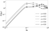 |
Fig. 1 Ratio of accretion onto the secondary and primary stars, λ = ṁs/ ṁp, plotted against the binary mass ratio, qb = ms/mp. The data are merged from Siwek et al. (2023) for qb > 0.1 and from Eq. (10) which is adapted from Kelley et al. (2019). The plot extends towards qb = 0 but is truncated for clarity. |
3 Modelling star formation
To explore the impact of preferential accretion, we used a molecular cloud model that has been extensively tested and validated by Haugbølle et al. (2018), and previously used in studies of multiplicity statistics (Kuruwita & Haugbølle 2023), stellar evolution (Jensen & Haugbølle 2018), and accretion (Pelkonen et al. 2021). A follow-up simulation with an identical setup but higher resolution also formed the basis for studies investigating water deuteration in stellar clusters (Jensen et al. 2021), and the role of post-collapse (late) infall in the star-formation process (Kuffmeier et al. 2023, 2024; Pelkonen et al. 2025). The physical domain of the molecular cloud is a periodic box of Lbox = 4 pc with a total mass of Mbox = 3000 M⊙. In addition, we assumed an isothermal sound speed of cs = 0.18 km s−1, which corresponds to T ≈ 10 K, and a mean molecular weight of µ = 2.37, which is a good approximation for a cold molecular cloud. The mean number density is nmean = 795 cm−3. The virial parameter was chosen such that the molecular cloud there is a balance between kinetic energy and gravitational energy, αvir = 0.83. The mean magnetic field strength is set to 7.2 = µG. Finally, the dynamical and free-fall times based on these parameters are tdyn = 1.08 Myr and tff = 1.18 Myr. Compared to observations, the adopted conditions are similar to those in the star-forming region of Perseus (Arce et al. 2010; Kuruwita & Haugbølle 2023).
The adaptive mesh was refined according to density and refinement is triggered when ρ > ρmax(ℓ), where ρmax(ℓ) is the maximum density for a given level, ℓ, and is given by Eq. (14):
 (14)
(14)
where ρlevelmin is the density of the minimum level, ∆x is the cell size, and ∆xmin is the cell size of the minimum level. Given the isothermal equation of state, this corresponds to keeping the Jeans length resolved by at least 28 cells at all refinement levels, except the highest, to suppress artificial fragmentation (Truelove et al. 1997).
The maximum level of refinement used to obtain the sample of stars is levelmax= 14, which corresponds to a cell size of  . Using this data set as the basis, we carried out higher resolution simulations, similar to zoom-in simulations (for more details see Kuffmeier et al. 2017), but applied globally in the box, to study the accretion process for eight selected sink pairs for stretches of 5 kyr, at resolutions up to levelmax=18 (corresponding to ∆x ≈ 3 AU).
Binary pair information.
4 Results
As part of validating the preferential accretion method, we performed a self-consistency test, since the preferential accretion method is based on idealised simulations of black holes and theoretical models of active galactic nuclei. For star formation, many interactions occur in a global simulation, and the gas in the larger-scale environment plays an important role; therefore, it is crucial to test the method. We also performed numerical convergence tests at increasingly higher resolution, continuing until the individual binary systems became fully resolved. This approach made a direct comparison of binary accretion rates possible obtained using the standard recipe and the newly developed algorithm of preferential binary accretion. From these simulations, we identified approximately 40 binary pairs and selected those with a minimum periastron greater than 0.25 cells and a maximum apastron smaller than 2.3 cells at levelmax = 14. This criterion ensures that the pairs are mostly or completely resolved at levelmax = 18, so that preferential accretion is inactive at this higher resolution. Details of the eight selected pairs can be found in Table 1. The key results are described in the following sections. For clarity, we only show and discuss the key results of using the new recipe for the binary pair comprising sinks 257 and 260. Equivalent plots for the remaining seven binary pairs are provided in the Appendix, corresponding to those shown in Figs. 2 and 4. The sinks are ordered by their creation time; for example, sink 257 is the 257th sink particle that formed, and sink 260 is the 260th.
4.1 Eliminating unphysical suppression of accretion
The new prescription eliminates the unphysical suppression of accretion that affected most binary systems with small separations in previous simulations, particularly at periastron. The unphysical accretion was a result of Eq. (6), which produces spurious fluctuations in the accretion rates for tight binaries, especially those located within the same cell. Similar effects are likely present in other codes that base accretion efficiency on an energy criterion and/or the relative velocity between gas cells and sink particles. This occurs because the older sink accretes most of the available material, leaving little or no material for accretion onto the younger sink, which usually corresponds to the lower-mass secondary star. We show an example of this in Fig. 2. The example illustrates the binary pair consisting of sinks 257 and 260, which have a mean separation of 1.4 cells at the maximum refinement level of levelmax = 14 in the reference run without activation of the new algorithm. The accretion rates for the other seven binary pairs studied (see Table 1) can be found in the appendix. Without the new recipe, the sink accretion rate of the primary (sink 257) varies by a factor of a few during each of the nearly eight orbits displayed over the 5 kyr time evolution. The accretion rate of the secondary (sink 260) varies by more than a factor of ten during some orbits.
In contrast, the accretion rates become much smoother and more regular when the new accretion recipe is applied. The top panel in Fig. 2 shows the total accretion rate, demonstrating that the preferential accretion algorithm maintains a total accretion rate comparable to that in the reference run but without the spurious dips at periastron. The accretion rate of the primary is systematically lower (middle panel), while that of the secondary is systematically higher (lower panel) compared with the reference run without the new recipe. This is a consequence of the underlying idealised scenarios of the binary accretion models that are used to derive the values of λ(q). In these scenarios, the lower-mass object (i.e. the secondary) moves through the denser gas, and thus accretes more material as it orbits the more massive primary. This effect is most pronounced for binary pairs with low q, i.e. sink pairs with large mass differences between the primary and secondary. For binaries with similar masses (sink pairs 75–82, 142–144, 217–221, and 253–254), this effect is less pronounced (Fig. A.2). For the nearly equal-mass pair (253– 254), the overall accretion rates of the primary and secondary closely match those in the runs without the recipe, except for the crucial improvement of quenching the spurious accretion dips at periastron. When the algorithm is active, the accretion rate shows little variability over the 5 kyr time interval, consistent with the accretion rates of single sinks in similar regions. In this example, the sinks are located within 0.7–1.9 cells of each other during the 5 kyr time interval. Increasing the resolution by a few refinement levels eliminates the unphysical suppression of accretion, even without activating the new recipe, as shown in the following subsection.
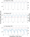 |
Fig. 2 Total and individual accretion rates for the pair 257, 260 at levelmax = 14. The results from the original algorithm are shown in blue, while the evolution using the new algorithm is shown in red. The sink pair exhibits order-of-magnitude variations in the individual accretion rates over an orbit with the original algorithm. The distance between the sinks (in AU) is shown as a dashed line and indicated on the right-hand y-axis. The pair has an average eccentricity of 0.5 and a mass ratio of 0.9. |
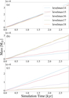 |
Fig. 3 Total (a), primary (b), and secondary (c) integrated masses of the sink pair 257, 260 at different resolutions from levelmax = 14 to 18. The origin is set to the point where the levelmax = 18 run begins. |
4.2 Resolution study
This resolution study aims to verify that the preferential accretion algorithm performs as intended at all resolutions where the binary pairs remain unresolved and to better understand its limitations. Fig. 4 reveals that the accretion rate increases with resolution for the primary sinks, whereas the opposite is true for the secondary sinks, where the lowest resolution run has the highest accretion rate. The higher primary and lower secondary accretion rates in the high-resolution runs, compared with the low-resolution runs where the recipe is active, result from a discrepancy between the accretion dynamics resolved in the zoom-in simulations and the assumption of an isolated circumbinary disc reservoir. Figure 5 shows the significant variations of λ, especially for values of q < 0.5. We intentionally show the case of sink 257–260, which exhibits the most significant differences in λ across the various resolutions. The example clearly illustrates the caveat of the preferential accretion algorithm. Its performance depends on how closely the dynamics of the specific protostellar pair match the idealised scenario that was used to compute the tabulated values. In this study, we adopted values for λ that were computed from an idealised scenario of binary accretion from a circumbinary disc. However, protostars are embedded in turbulent molecular cloud environments with more complicated overall dynamics (Fig. 6). The resolution study reveals that the primary (secondary) sink accretes more (less) material than in the idealised scenario of accretion from an isolated circumbinary disc. Moreover, the primary star systematically accretes less material than younger binary systems, particularly for pairs with significant mass differences between the two components.
In addition to this, the lower-resolution runs show smoother total accretion profiles with less dependence on separation, consistent with the expectations of increased complexity when the system is more resolved. Nevertheless, the accretion rates vary by less than an order of magnitude, indicating that we obtain a good approximation without resolving the system. An interesting behaviour is evident in the levelmax = 16 run: near periastron, it aligns almost perfectly with the accretion rates at lower resolutions, while elsewhere it aligns with the higher resolutions. This occurs because, at this resolution, the binary is only partially resolved, such that for most of the time their accretion radii do not overlap sufficiently to activate the binary accretion recipe. Near periastron, however, the overlap is large enough for the binary accretion recipe to dominate the accretion.
Examining the integrated mass of this system over the same time interval in Fig. 3, we find similar behaviour for the primary and secondary sinks. For the total integrated mass, we clearly see that the accretion rate is comparable for this system, regardless of whether preferential accretion is active or whether the system is gradually being resolved. This consistency is less clear for several of the other systems, where there is some variation. This is likely due to the complexity and turbulence of the environments surrounding the binary systems. This aspect is explored in more detail in the following section.
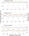 |
Fig. 4 Total (a), primary (b), and secondary (c) accretion rates for the sink pair 257, 260 at different resolutions from levelmax = 14–18. The distance between the sinks, in AU, is shown on the right-hand y-axis. The pair has an average eccentricity of 0.5 and a mass ratio of 0.9. |
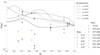 |
Fig. 5 Average λ of each pair in each run as a function of the mass ratio. The colour indicates the resolution of the run, and the symbol identifies which pair it represents. The lines are the same as those in Fig. 1. |
4.3 Idealised algorithm in a complex and turbulent environment
Figure 5 shows the average value of λ, providing a basis for a direct comparison between the simulation results and the theoretical relation presented in Fig. 1. The results exhibit a large spread, with only a subset of points agreeing with the theoretical model. This represents an important limitation: the algorithm is not perfect, and in real complex situations, other factors affect the accretion. Regardless of the resolution, Fig. 6 illustrates the complexity of the turbulent environment. In the complementary Fig. 5, the average λ, without the theoretical curve, is shown to visualise each pair and the run from which it originates. Some pairs, such as 257–260 discussed above, exhibit a large spread in λ, whereas others, such as 75–82 and 292–290, show much smaller variations. This demonstrates that all selected pairs have different characteristics within the imposed constraints, and also implies that exact similarity cannot be expected.
5 Discussion
We have successfully eliminated the unphysical suppression of accretion in unresolved close binaries, which was the main shortcoming of previous accretion approaches. This effect is evident across all figures in the resolution study, particularly in Fig. 2, where we observe that the maximum difference is twice the minimum value. For most cases, the variability generally remains below 0.4, representing a substantial improvement compared with runs that do not include a binary sub-sink accretion algorithm. We find that the variability increases for levelmax = 17 and 18, which is due to a more complicated environment around the binary system, as shown in Fig. 6, where, for example, the individual discs and outflows begin to be marginally resolved.
The systematic offset in accretion variability observed in the low-resolution runs without activation of the new sink algorithm has a significant impact. Most simulation codes employ a similar method of accretion without incorporating a recipe for preferential accretion and consequently exhibit unphysical suppression of accretion for tight binaries. We demonstrate that this artificial quenching of accretion can be eliminated using our new approach, which implements a simple, idealised framework for accretion onto binary black holes and active galactic nuclei. This implies that future simulations can perform global runs while still obtaining reliable accretion rates for binary systems at lower resolution than would be possible without the new algorithm. This is helpful for investigating binaries in large-scale simulations, because larger and/or longer simulations can be run at lower cost, facilitating a better understanding of the accretion process in entire star-forming regions. We find that lower-resolution simulations produce more even accretion rate curves, while the average accretion rates remain similar across resolutions. These lower-resolution simulations exhibit less variability and correspondingly flatter accretion profiles. This likely arises because, as resolution increases, the surroundings become better resolved and more complex structures, such as discs and outflows, begin to appear. Some of these structures can be seen in Fig. 6, as well as in the high-resolution column density maps of the other binary pairs shown in Figs. A.3 to A.9. These structures can significantly influence the accretion process (see review by Tsukamoto et al. 2023, and references therein), including the launching of outflows (Podio et al. 2021).
In a more detailed analysis, the mass fractions accreted by the sink particles appear to be well converged for mass ratios close to unity. This is particularly evident in Fig. 5, where the two highest mass-ratio pairs show good agreement in λ across resolutions. This also agrees with expectations that for a mass ratio approaching unity, λ approaches unity. We also find a large spread in λ for lower mass ratios. Specifically, the primary star accretes significantly more than the secondary, in the region where the idealised model predicts the opposite. However, these cases occur at higher resolution when the binary accretion recipe is not active or is only partially active. The key takeaway is that binary accretion for low mass ratios (q) remains poorly understood, and further work is required to characterise this regime for proto-binaries in gas-rich environments.
In this study, our analysis is limited to eight binary systems, which does not fully cover the parameter space required to characterise the spread of λ with mass ratio and eccentricity. This work therefore represents a first presentation of the new preferential binary accretion recipe. The pairs were specifically chosen to be distinct from each other so that we could investigate the implications over the widest range of systems possible within our simulation data. Future research should investigate the impact of eccentricity on the accretion process in binary systems (such as studied by O’Neill et al. 2024), particularly in the context of star formation within turbulent regions.
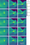 |
Fig. 6 Column density plot on the 3 axes of the primary sink particle in a 1000 AU by 1000 AU field of view, where the primary sink is the blue star and the secondary is the red star. The resolution goes from levelmax = 14 at the bottom panel to levelmax = 18 at the top in steps of 1. It shows the complex surroundings of pair 257, 260 and how with increasing resolution the gas flow to the individual sinks becomes mostly resolved. |
6 Conclusion
In this paper, we address accretion in unresolved binary systems. Existing accretion recipes introduce high time variability and rely on assumptions that cannot adequately capture the physical flow, such as preferential accretion onto the secondary star in the system. To overcome spurious accretion in binary systems, we introduce a new preferential binary accretion recipe, based on theoretical models from active galactic nuclei and idealised simulations of binary black holes. Its implementation in RAMSES aims to eliminate this unphysical accretion and achieve a better approximation of accretion in unresolved binary systems.
The new accretion recipe successfully eliminates the unphysical dips in accretion rates at periastron observed in runs without the recipe. This represents a significant improvement over current models and can easily be extended to codes beyond RAMSES, enabling a more accurate description of binary system accretion in global simulations. Additionally, our approach tracks the fraction of mass available for accretion by the binary components. This feature is particularly useful for close binaries, often located within the same cell at lower resolution, and it provides a reliable approximation of accretion for mass ratios close to unity. Together, these features enable global simulations to be run at lower resolution than would otherwise be required for binaries to provide usable data.
Although the algorithm is successful, it has limitations. The impact of eccentricity and mass ratio on accretion in binary systems at low mass ratios (∼0.1) remains unclear. Nevertheless, this work provides the first results illustrating accretion behaviour using the preferential accretion recipe. Our study shows that adopting accretion parameters derived from models of binary accretion in isolated circumbinary discs can lead to substantial differences for sink pairs that are actually embedded and affected by the turbulent molecular cloud environment. In particular, our resolution study shows that the accretion rate of the secondary tends to be overestimated when using tabulated values derived from isolated accretion models, compared with models where the embedded binary system is resolved. We suggest that obtaining accretion histories for more embedded binary sinks in molecular clouds could provide a more refined table of the adopted accretion parameters and thereby optimise the use of the recipe. Further work is required to determine how the recipe can be improved in this regime. Despite these limitations, this study represents an important step forward in modelling close binary systems, particularly in large-scale simulations, and in improving future constraints on the accretion histories of embedded binaries. By providing a more accurate and computationally efficient method, this work contributes to the broader effort to model and understand star-forming regions and protostellar binaries.
Data availability
A Fortran implementation of the binary accretion module, together with figures from this paper and additional column density images at different resolutions illustrating the physical and numerical processes, is available through University of Copenhagen Electronic Research Data Archive (ERDA)2. The bulk data generated and analysed in this paper are not publicly available due to their large volume and ongoing research on other aspects of the datasets; however, they are available upon reasonable request.
Acknowledgements
The Tycho HPC facility at the University of Copenhagen, supported by research grants from the Carlsberg, Novo, and Villum foundations, was used for carrying out the simulations, the analysis, and the long-term storage of the results. MK acknowledges funding from a Carlsberg Reintegration Fellowship (CF22-1014). TH acknowledges funding from the Independent Research Fund Denmark through grant No. DFF 4283-00305B.
References
- Arce, H. G., Borkin, M. A., Goodman, A. A., Pineda, J. E., & Halle, M. W. 2010, ApJ, 715, 1170 [NASA ADS] [CrossRef] [Google Scholar]
- Bate, M. R., Bonnell, I. A., & Price, N. M. 1995, MNRAS, 277, 362 [Google Scholar]
- Belyakov, V. A., Filatov, O. G., Grigoriev, S. A., Sytchevsky, S. E., & Tanchuk, V. N. 2004, Plasma Devices Oper., 12, 103 [Google Scholar]
- Bleuler, A., & Teyssier, R. 2014, MNRAS, 445, 4015 [Google Scholar]
- Connelley, M. S., Reipurth, B., & Tokunaga, A. T. 2008, AJ, 135, 2496 [Google Scholar]
- Duquennoy, A., & Mayor, M. 1991, A&A, 248, 485 [NASA ADS] [Google Scholar]
- Farris, B. D., Duffell, P., MacFadyen, A. I., & Haiman, Z. 2014, ApJ, 783, 134 [NASA ADS] [CrossRef] [Google Scholar]
- Federrath, C., Banerjee, R., Clark, P. C., & Klessen, R. S. 2010, ApJ, 713, 269 [NASA ADS] [CrossRef] [Google Scholar]
- Federrath, C., Schrön, M., Banerjee, R., & Klessen, R. S. 2014, ApJ, 790, 128 [NASA ADS] [CrossRef] [Google Scholar]
- Fromang, S., Hennebelle, P., & Teyssier, R. 2006, A&A, 457, 371 [NASA ADS] [CrossRef] [EDP Sciences] [Google Scholar]
- Gong, H., & Ostriker, E. C. 2013, ApJS, 204, 8 [NASA ADS] [CrossRef] [Google Scholar]
- Grudić, M. Y., Guszejnov, D., Hopkins, P. F., Offner, S. S. R., & Faucher-Giguère, C.-A. 2021, MNRAS, 506, 2199 [NASA ADS] [CrossRef] [Google Scholar]
- Haugbølle, T., Padoan, P., & Nordlund, Å. 2018, ApJ, 854, 35 [CrossRef] [Google Scholar]
- Hopkins, P. F. 2015, MNRAS, 450, 53 [Google Scholar]
- Hubber, D. A., Walch, S., & Whitworth, A. P. 2013, MNRAS, 430, 3261 [NASA ADS] [CrossRef] [Google Scholar]
- Jensen, S. S., & Haugbølle, T. 2018, MNRAS, 474, 1176 [Google Scholar]
- Jensen, S. S., Jørgensen, J. K., Furuya, K., Haugbølle, T., & Aikawa, Y. 2021, A&A, 649, A66 [NASA ADS] [CrossRef] [EDP Sciences] [Google Scholar]
- Kelley, L. Z., Haiman, Z., Sesana, A., & Hernquist, L. 2019, MNRAS, 485, 1579 [NASA ADS] [CrossRef] [Google Scholar]
- Krumholz, M. R., McKee, C. F., & Klein, R. I. 2004, ApJ, 611, 399 [NASA ADS] [CrossRef] [Google Scholar]
- Kuffmeier, M., Haugbølle, T., & Nordlund, Å. 2017, ApJ, 846, 7 [NASA ADS] [CrossRef] [Google Scholar]
- Kuffmeier, M., Frimann, S., Jensen, S. S., & Haugbølle, T. 2018, MNRAS, 475, 2642 [NASA ADS] [CrossRef] [Google Scholar]
- Kuffmeier, M., Jensen, S. S., & Haugbølle, T. 2023, Eur. Phys. J. Plus, 138, 272 [NASA ADS] [CrossRef] [Google Scholar]
- Kuffmeier, M., Pineda, J. E., Segura-Cox, D., & Haugbølle, T. 2024, A&A, 690, A297 [NASA ADS] [CrossRef] [EDP Sciences] [Google Scholar]
- Kuruwita, R. L., & Haugbølle, T. 2023, A&A, 674, A196 [NASA ADS] [CrossRef] [EDP Sciences] [Google Scholar]
- Lai, D., & Muñoz, D. J. 2023, ARA&A, 61, 517 [Google Scholar]
- Offner, S. S. R., Taylor, J., Markey, C., et al. 2022, MNRAS, 517, 885 [NASA ADS] [CrossRef] [Google Scholar]
- O’Neill, D., D’Orazio, D. J., Samsing, J., & Pessah, M. E. 2024, arXiv e-prints [arXiv:2401.16166] [Google Scholar]
- Padoan, P., Haugbølle, T., & Nordlund, Å. 2014, ApJ, 797, 32 [Google Scholar]
- Pelkonen, V. M., Padoan, P., Haugbølle, T., & Nordlund, Å. 2021, MNRAS, 504, 1219 [NASA ADS] [CrossRef] [Google Scholar]
- Pelkonen, V. M., Padoan, P., Juvela, M., Haugbølle, T., & Nordlund, Å. 2025, A&A, 694, A327 [NASA ADS] [CrossRef] [EDP Sciences] [Google Scholar]
- Pineda, J. E., Arzoumanian, D., Andre, P., et al. 2023, in Astronomical Society of the Pacific Conference Series, 534, Protostars and Planets VII, eds. S. Inutsuka, Y. Aikawa, T. Muto, K. Tomida, & M. Tamura, 233 [NASA ADS] [Google Scholar]
- Podio, L., Tabone, B., Codella, C., et al. 2021, A&A, 648, A45 [NASA ADS] [CrossRef] [EDP Sciences] [Google Scholar]
- Raghavan, D., McAlister, H. A., Henry, T. J., et al. 2010, ApJS, 190, 1 [Google Scholar]
- Siwek, M., Weinberger, R., Muñoz, D. J., & Hernquist, L. 2023, MNRAS, 518, 5059 [Google Scholar]
- Springel, V. 2010, MNRAS, 401, 791 [Google Scholar]
- Truelove, J. K., Klein, R. I., McKee, C. F., et al. 1997, ApJ, 489, L179 [CrossRef] [Google Scholar]
- Tsukamoto, Y., Maury, A., Commercon, B., et al. 2023, in Astronomical Society of the Pacific Conference Series, 534, Protostars and Planets VII, eds. S. Inutsuka, Y. Aikawa, T. Muto, K. Tomida, & M. Tamura, 317 [Google Scholar]
- Vorobyov, E. I., Elbakyan, V. G., Liu, H. B., & Takami, M. 2021, A&A, 647, A44 [EDP Sciences] [Google Scholar]
- Wurster, J., & Lewis, B. T. 2020, MNRAS, 495, 3807 [CrossRef] [Google Scholar]
Appendix A Evolution of binary pairs
To demonstrate the different accretion profiles of the binary pairs, we show the accretion rates for the other six pairs without and with the implementation of our new algorithm for the different resolutions in Figs. A.1 and A.2. The figures are complementary to the ones shown for the reference sink pair 257/260. Similarly, we illustrate the various protostellar environments in the column density maps of the binary systems in Fig. A.3 to Fig. A.9, complementary to the column density map shown for the reference sink pair 257/260 in Fig. 6.
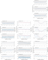 |
Fig. A.1 Same as Fig. 2 but for sink pairs 75/82, 141/146, 142/144, 217/219, 253/254, 279/281, and 292/290. |
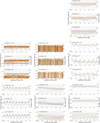 |
Fig. A.2 Same as Fig. 4 but for sink pairs 75/82, 141/146, 142/144, 217/219, 253/254, 279/281, and 292/290. |
All Tables
All Figures
|
Fig. 1 Ratio of accretion onto the secondary and primary stars, λ = ṁs/ ṁp, plotted against the binary mass ratio, qb = ms/mp. The data are merged from Siwek et al. (2023) for qb > 0.1 and from Eq. (10) which is adapted from Kelley et al. (2019). The plot extends towards qb = 0 but is truncated for clarity. |
| In the text | |
|
Fig. 2 Total and individual accretion rates for the pair 257, 260 at levelmax = 14. The results from the original algorithm are shown in blue, while the evolution using the new algorithm is shown in red. The sink pair exhibits order-of-magnitude variations in the individual accretion rates over an orbit with the original algorithm. The distance between the sinks (in AU) is shown as a dashed line and indicated on the right-hand y-axis. The pair has an average eccentricity of 0.5 and a mass ratio of 0.9. |
| In the text | |
|
Fig. 3 Total (a), primary (b), and secondary (c) integrated masses of the sink pair 257, 260 at different resolutions from levelmax = 14 to 18. The origin is set to the point where the levelmax = 18 run begins. |
| In the text | |
|
Fig. 4 Total (a), primary (b), and secondary (c) accretion rates for the sink pair 257, 260 at different resolutions from levelmax = 14–18. The distance between the sinks, in AU, is shown on the right-hand y-axis. The pair has an average eccentricity of 0.5 and a mass ratio of 0.9. |
| In the text | |
|
Fig. 5 Average λ of each pair in each run as a function of the mass ratio. The colour indicates the resolution of the run, and the symbol identifies which pair it represents. The lines are the same as those in Fig. 1. |
| In the text | |
|
Fig. 6 Column density plot on the 3 axes of the primary sink particle in a 1000 AU by 1000 AU field of view, where the primary sink is the blue star and the secondary is the red star. The resolution goes from levelmax = 14 at the bottom panel to levelmax = 18 at the top in steps of 1. It shows the complex surroundings of pair 257, 260 and how with increasing resolution the gas flow to the individual sinks becomes mostly resolved. |
| In the text | |
|
Fig. A.1 Same as Fig. 2 but for sink pairs 75/82, 141/146, 142/144, 217/219, 253/254, 279/281, and 292/290. |
| In the text | |
|
Fig. A.2 Same as Fig. 4 but for sink pairs 75/82, 141/146, 142/144, 217/219, 253/254, 279/281, and 292/290. |
| In the text | |
 |
Fig. A.3 Same as Fig. 6 but for pair 75/82. |
| In the text | |
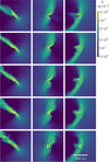 |
Fig. A.4 Same as Fig. 6 but for pair 141/146. |
| In the text | |
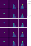 |
Fig. A.5 Same as Fig. 6 but for pair 142/144. |
| In the text | |
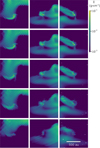 |
Fig. A.6 Same as Fig. 6 but for pair 217/219. |
| In the text | |
 |
Fig. A.7 Same as Fig. 6 but for pair 253/254. |
| In the text | |
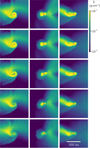 |
Fig. A.8 Same as Fig. 6 but for pair 279/219. |
| In the text | |
 |
Fig. A.9 Same as Fig. 6 but for pair 290/292. |
| In the text | |
Current usage metrics show cumulative count of Article Views (full-text article views including HTML views, PDF and ePub downloads, according to the available data) and Abstracts Views on Vision4Press platform.
Data correspond to usage on the plateform after 2015. The current usage metrics is available 48-96 hours after online publication and is updated daily on week days.
Initial download of the metrics may take a while.