| Issue |
A&A
Volume 708, April 2026
|
|
|---|---|---|
| Article Number | A333 | |
| Number of page(s) | 6 | |
| Section | The Sun and the Heliosphere | |
| DOI | https://doi.org/10.1051/0004-6361/202659038 | |
| Published online | 21 April 2026 | |
Cyclic sunspot activity during the first millennium CE as reconstructed from radiocarbon
1
Space Physics and Astronomy research Unit, Sodankylä Geophysical Observatory, University of Oulu, Oulu, Finland
2
Max-Planck Institute for Solar System Research, Justus-von-Liebig-Weg 3, 37077 Göttingen, Germany
3
Institute for Space-Earth Environmental Research, Nagoya University, Furo-cho, Chikusa-ku, Nagoya 464-8601, Japan
★ Corresponding author: This email address is being protected from spambots. You need JavaScript enabled to view it.
Received:
19
January
2026
Accepted:
16
March
2026
Abstract
Context. Solar activity, dominated by 11-year cyclic evolution, has been observed directly since 1610 CE. Indirect cosmogenic proxy data have been used to reconstruct solar activity for millennia prior to 1610. The precision of radiocarbon Δ14C measurements has recently improved enough to allow cyclic solar activity to be reconstructed over millennia.
Aims. We present the first detailed reconstruction of solar activity, represented here by annual sunspot numbers, during the first millennium, 1–969 CE.
Methods. The reconstruction of sunspot numbers from Δ14C was performed using a physics-based method that involves several steps: First, using the modern carbon-cycle box model, the 14C production rate, corrected for the contemporary geomagnetic shielding, was computed from the measured concentrations. The open solar magnetic flux was then computed using a model of the heliospheric cosmic-ray modulation. Sunspot numbers were calculated by inverting a model of the evolution of the Sun’s magnetic field. Lastly, the Markov chain Monte Carlo approach was used to directly account for different sources of uncertainty.
Results. Annual sunspot numbers were reconstructed for the first millennium CE. This period includes one extreme solar event that occurred in 774 CE and one grand solar minimum, from 650 to 730 CE. We were able to identify 91 solar cycles, of which 26 were well defined, 24 were reasonably well defined, and 41 were poorly defined. The mean cycle length was 10.6 years, but the lengths of individual cycles vary between 8 and 15 years. The existence of empirical Waldmeier relations remains inconclusive with this dataset. No significant periodicities were found beyond the 11-year cycle.
Conclusions. This work fills the gap in the solar cycle statistics between the previously reconstructed first millennium BCE and the second millennium CE, providing vital constraints for solar dynamo and irradiance models. A consistent 3-millennium-long reconstruction of sunspot numbers, based on a composite multi-proxy cosmogenic record, is pending.
Key words: Sun: activity / solar-terrestrial relations / sunspots
© The Authors 2026
 Open Access article, published by EDP Sciences, under the terms of the Creative Commons Attribution License (https://creativecommons.org/licenses/by/4.0), which permits unrestricted use, distribution, and reproduction in any medium, provided the original work is properly cited.
This article is published in open access under the Subscribe to Open model. This email address is being protected from spambots. You need JavaScript enabled to view it. to support open access publication.
1. Introduction
The Sun is a variable star. This variability is an important driver of the terrestrial environment (e.g. Gray et al. 2010; Haigh et al. 2010) and serves as a laboratory for testing solar and/or stellar dynamo theory (e.g. Charbonneau 2020; Karak 2023). Solar magnetic activity is dominated by quasi-periodicity with a roughly 11-year timescale (Hathaway 2015), called the Schwabe cycle. The Schwabe cycle is strongly modulated by secular variability, ranging from periods of very low solar activity, known as grand minima (the most recent being the Maunder minimum between 1645 and 1715; Eddy 1976; Usoskin et al. 2015), to periods of very high solar activity, called grand maxima, such as in the second half of the 20th century (Usoskin et al. 2003; Solanki et al. 2004). However, the statistical properties of solar grand minima and maxima are poorly constrained by direct sunspot observations. Several empirical rules describe solar cycle characteristics, such as Waldmeier’s rule (Waldmeier 1939), which relates the strength of a solar cycle to the length of its rising phase. These relations were inferred from direct instrumental observations of sunspots over the last four centuries, covering only 25 reasonably resolved cycles and a dozen additional, more poorly constrained ones (Clette & Lefèvre 2016). Consequently, the statistical significance of such empirical relations remains limited.
Indirect proxies in the form of cosmogenic isotopes, mostly 14C measured in tree rings and 10Be in ice cores, made it possible to reconstruct solar activity on a multi-millennial timescale over the Holocene (e.g. Solanki et al. 2004; Vonmoos et al. 2006; Steinhilber et al. 2012; Beer et al. 2012; Wu et al. 2018). However, this method, while reliably reconstructing long-term variability, could not resolve individual solar cycles due to the insufficient temporal resolution of isotope measurements (e.g. Usoskin 2023). For example, although several dozen grand minima and maxima were found during the Holocene (Usoskin et al. 2007; Inceoglu et al. 2015), the behaviour of very low solar activity was known only for the Maunder minimum (e.g. Vaquero et al. 2015).
A major breakthrough in the quality of 14C measurements was made recently, thanks to the development of accelerator mass spectrometry, which has made it possible to reconstruct individual solar cycles from annual tree-ring data (see a review by Heaton et al. 2024). The first of this kind was a precision set of annual 14C measurements covering the last millennium (Brehm et al. 2021). A careful analysis of this dataset allowed us to reconstruct 85 individual sunspot cycles for the period 970–1900 CE (Usoskin et al. 2021). A similar-precision dataset for the first millennium BCE (Brehm et al. 2025) led to a reconstruction of 93 solar cycles from that period (Usoskin et al. 2025). These results provide important constraints on solar dynamo theory (e.g. Biswas et al. 2023).
Very recently, the millennium-long gap between the previously measured annual-resolution datasets has been bridged by a high-resolution 14C dataset covering the first millennium CE (Wang et al. 2026). By applying the methodology developed by us earlier (Usoskin et al. 2021, 2025) to this new dataset, we reconstructed individual sunspot cycles for the period 1–970 CE and present the results of their statistical analysis.
2. Data
Several datasets have been used in this work. Our main dataset comprises the series of the relative concentration of radiocarbon 14C measured at an annual resolution in European oak trees for the period 1–969 CE (Wang et al. 2026). It is shown in Fig. 1a along with 1σ error bars, which are of the order of 1.6%. The errors are mostly defined by the measurement uncertainties of individual tree-ring samples, which are independent between measurements. Most of the data points are based on single-tree samples. For intervals with multiple measurement points, a weighted average was used to obtain annual values and their uncertainties. Possible non-Gaussian errors during periods with multiple tree sample measurements were not taken into consideration. The dataset includes several short gaps (data from the years 475, 573, 804, 805, 809, 928, 929, 944, and 945 CE were missing), which were linearly interpolated, and an enhanced error bar of σ = 5% was assigned to the interpolated data points.
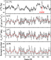 |
Fig. 1. Sequential steps of the annual solar activity reconstructions for the first millennium CE. Panel (a): raw Δ14C data (Wang et al. 2026). The red arrow indicates the signature of the ESPE of 774 CE. Panel (b): 14C production rate (Q*) corrected for geomagnetic shielding and ESPE effects. Panel (c): OSF (Fo). Panel (d): SN. Black curves, grey shading, and red curves depict the annual values, 1σ (68% confidence interval) uncertainties, and 22-year smoothed data, respectively. |
Since the reconstruction of solar activity from cosmogenic isotopes involves correction for the geomagnetic shielding, we considered six recent archeo- and/or paleo-magnetic models that cover the period of interest in the form of the virtual dipole moment (VDM), as shown in Fig. 2. As seen, the geomagnetic field was stable and strong (VDM is in the range (9–11) ⋅ 1022 A m2) and is bounded by the AK and K08 curves.
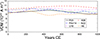 |
Fig. 2. Recent reconstructions of the geomagnetic VDM for the first millennium CE. The models are P23 (Panovska et al. 2023), K08 (Knudsen et al. 2008), PAV14 (Pavón-Carrasco et al. 2014), N22 (Nilsson et al. 2022), U16 (Usoskin et al. 2016), and AK (Schanner et al. 2022). |
While the radiocarbon production is mostly defined by the Galactic cosmic rays, very roughly once per millennium the Sun produces extreme solar particle events (ESPEs) that are observable as distinct increases in Δ14C (e.g. Miyake et al. 2012; Usoskin et al. 2013; Cliver et al. 2022). While an ESPE leads to a nearly instantaneous production of a large amount of 14C in the atmosphere, its signature in the measured concentration Δ14C can spread over a decade, distorting the solar activity signal (e.g. Miyake et al. 2020). If unaccounted for, the enhanced 14C production is interpreted by the reconstruction method as a weak (or even unphysically negative) sunspot number (SN), as shown in Fig. 3. Accordingly, the ESPE needs to be de-trended from the dataset before further analysis. The analysed dataset contains one known ESPE, from 774 CE (Miyake et al. 2012), as denoted in Fig. 1a. It was de-trended, as illustrated in Fig. 3a. This was done by removing the modelled ESPE signal (dashed blue line) from the raw Δ14C to obtain the de-trended data (dot-dashed red curve), similar to the approach by Usoskin et al. (2025). The modelled ESPE curve was computed using the SOCOL:14C-Ex model (Golubenko et al. 2025). Although the raw-data uncertainties were directly translated to the de-trended dataset, the affected reconstructed solar cycles are considered to be of low quality.
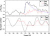 |
Fig. 3. Correction of the dataset for the ESPE of 774 CE. Panel (a): mean raw Δ14C annual data (black curve), the modelled 774 response (dashed blue lines; T = 130 DoY, A = 3.5; see Golubenko et al. 2025), and de-trended Δ14C data (dash-dotted red curve). Panel (b): SNs reconstructed from the raw Δ14C (black) and de-trended (red) datasets. Error bars are omitted for clarity in all panels. |
3. Methodology
3.1. Reconstruction
The SN reconstruction was performed following the methodology we developed for a similar task earlier (see Usoskin et al. 2021, 2025 for details). The reconstruction method is based on the Markov chain Monte Carlo (MCMC) approach and uses 10000 ensemble reconstructions. It is composed of four consecutive steps, each involving its own source of uncertainties:
 (1)
(1)
Here Q is the 14C production rate, Q* is the same after correcting for the shielding by the geomagnetic field, and Fo is the open magnetic flux. Before processing, the dataset was corrected for the effect of the 774 CE ESPE as described above.
In Step 1, for the j-th year and i-th ensemble realisation, the annual Δ14C value was taken as
 (2)
(2)
where ⟨Δ⟩j and σΔj are the mean and the uncertainty of the radiocarbon data for the j-th year, and R is a normally distributed random number with zero mean and unit dispersion. Before further analysis, the simulated data series for each realisation was smoothed with a low-pass filter (lowpass Matlab routine with a normalised passband frequency wc = 0.17, corresponding to about three years) to avoid the amplification of noise, as discussed in detail in Usoskin et al. (2025). Then, the 14C production rate (Qi, j) was computed from these Δ14C values by applying the multi-box carbon cycle model (Güttler et al. 2015; Büntgen et al. 2018). In this way, 10 000 ensemble series of Qi.j were obtained. This production rate (Q) is close to that obtained by Wang et al. (2026).
In Step 2, the production rates (Q) computed in Step 1 were translated to those corresponding to the current conditions (VDM = 7.75 ⋅ 1022 A m2), denoted as Q*. The translation was made using the calibration curve from Usoskin et al. (2021). For each ensemble realisation (i), one VDM model was randomly chosen from the six considered models (see Fig. 2) for all years. The evolution of Q* is shown in Fig. 1b. It varies between 1.2 and 2 atom cm−2 s−1, with a mean value of about 1.6 atom cm−2 s−1.
In Step 3, we converted the geomagnetically corrected production rate (Q*) into the open solar flux (OSF; Fo) by applying a physics-based model (Usoskin et al. 2021, 2025), which also includes an additive uncertainty term: σF = 0.9 ⋅ 1014 Wb. The evolution of the OSF is shown in Fig. 1c. It varies in the range (2 − 10)⋅1014 Wb, with a mean value of about 5.9 × 10¹⁴ Wb. We note that the modulation parameter is often derived from cosmogenic-isotope data (e.g. Brehm et al. 2021; Wang et al. 2026). However, since it is ambiguously defined depending on the assumed local interstellar spectrum of Galactic cosmic rays (e.g. Usoskin et al. 2005; Herbst et al. 2010), we used a physically better defined OSF quantity here.
In Step 4, we computed SNs from the OSF (Fo) by applying an empirical conversion algorithm developed by Usoskin et al. (2021). The ensemble SN reconstruction is shown in Fig. 1d. The dominant cyclic variability is clearly seen. It is analysed in the next section.
3.2. Uncertainties of the reconstruction
There are several sources of uncertainty in the SN reconstruction. The MCMC method enables a direct estimation of error propagation in the reconstruction, allowing for the individual switching of different uncertainty sources. The contributions of different processes to the summary uncertainty of the SN reconstruction are shown in Fig. 4 as computed for 1000 ensemble realisations. The total 1σ uncertainty (green line) varies between 20 and 70 in SN, depending on the solar activity level. The total uncertainty is dominated by the radiocarbon measurement errors, which are comparable to the solar cycle amplitude in Δ14C, as indicated by the red line. The uncertainties related to the paleo-magnetic reconstructions are modest, 10–20 SNs, because of the fairly stable and large geomagnetic dipole strength over that period. The uncertainty of the model, which includes both the production rate-to-OSF and OSF-to-SN conversions, remains stable at about 15 SN units (cf. Usoskin et al. 2025). Since the sources of uncertainty are independent of each other, the total uncertainty is very close to the geometrical sum of the individual uncertainties. As seen, the reconstructed SN is uncertain for SNs < 50, while for strong cycles, the uncertainties reach about one-third of the SN value.
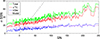 |
Fig. 4. Different sources of uncertainties of the SN reconstruction plotted at the 1σ level: radiocarbon measurement errors (red Δ14C line), geomagnetic models (blue VDM line), model uncertainties (magenta line) including both the computation of the OSF and the OSF-to-SSN conversion, and the total uncertainty (green line), which is close to the geometrical sum of the individual uncertainties. The dashed black line represents the diagonal. |
4. Results and analyses
4.1. Reconstructed sunspot numbers
The reconstructed SN series, in the International Sunspot Number (ISN) v.2 definition (Clette & Lefèvre 2016), is shown in Fig. 5. It is split into two panels for better visibility. The evolution is dominated by cyclic variations in activity, which are modulated on longer timescales. To highlight secular changes, we also show, as a red line, a smooth 22-year low-pass signal, which varies between nearly zero and 100 in SN units. The green line depicts the decadal SN reconstruction based on a multi-proxy approach (Wu et al. 2018). Unsurprisingly, the latter is smoother, being based on multi-isotope data, but shows a very similar level and long-term variability as the present reconstruction.
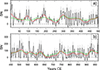 |
Fig. 5. SNs (ISN_v2 normalisation) reconstructed here for 1–969 CE, split into two panels for clarity. The black curve, grey shading, and red curve depict the mean annual reconstructed SN, its 68% confidence interval, and the 22-year smoothed evolution (see main text), respectively. These data are identical to those in Fig. 1d. The digital version of these data is available at the CDS. The green curve depicts the smooth decadal SN values reconstructed from multi-proxy cosmogenic isotope data (Wu et al. 2018). |
The analysed period contains one full grand minimum that occurred from 650–730 CE, called the Horrebow minimum (Kaiser Kudsk et al. 2022; Usoskin 2023). In addition, several shorter periods of weak activity can be observed circa 250 CE and 430 CE. However, no periods similar to the modern grand maximum, with the maximum SN systematically exceeding 200, appear in the reconstructed series. The solar activity level was more stable (11 weak cycles with ⟨SN⟩< 20) during the first millennium CE than during the first millennium BCE (16 weak cycles, two grand minima; Usoskin et al. 2025) and the second millennium CE (42 weak cycles, three grand minima; Usoskin et al. 2021). This implies that grand minima are not evenly distributed in time but tend to cluster over a multi-millennial scale (Usoskin et al. 2007, 2016).
A wavelet spectrum of the reconstructed sunspot series is shown in Fig. 6. The only significant periodicity is around 11 years, with a broad range of periods between 8 and 15 years. However, the 11-year periodicity appears insignificant around the periods of weak activity circa 150, 250, and 700 CE. Other notable, but not statistically significant, quasi-periodicities are found around 200 years (Suess or de Vries cycle), 70–140 years (Geissberg cycle), and 50 years.
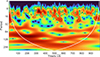 |
Fig. 6. Wavelet spectrum (Morlet basis, k = 6) of the reconstructed annual mean SN series. The black-contoured areas represent the statistically significant spectral power (p < 0.05 against the AR1 red noise). The white line bounds the cone of influence, below which the results are unreliable. |
4.2. Solar cycles
From the annually reconstructed SNs (Fig. 5), one can identify individual solar cycles. A total of 91 solar cycles were identified (see Table A.1). The quality of the reconstructed cycles is uneven and varies from poorly resolved to very clear solar cycles. To account for that, we used, similarly to previous studies (Usoskin et al. 2021, 2025), the quality flag (q) defined as follows:
-
The cycle cannot be identified, but only guessed, or its strength is consistent with zero at the 1σ level. Ten such cycles were found.
-
The cycle is strongly distorted, or its strength is consistent with zero at the 2σ level. The timing of cycle minima and maxima cannot be reliably defined. We found 12 such cycles.
-
The cycle can be approximately identified, but either its shape or level is distorted. The timing of cycle minima can be imprecise for several years, while the maximum can be undefined. We found 18 such cycles.
-
The cycle is reasonably well defined, but the minimum or maximum is not clear, or the cycle contains a gap longer than one year. We found 24 such cycles.
-
The cycle is clear in shape but has a somewhat unclear amplitude. We found 15 such cycles.
-
The cycle is clear in shape and amplitude. We found 11 such cycles.
Out of the 91 identified cycles, 26 are well defined (q > 3), 24 are reasonably well defined (q = 3), 30 are poorly defined (q = 1–2), and 10 are undefined or only guessed (q ≤ 1). The first and the last cycles could be affected by the edges of the data series.
With a total of 91 cycles over 970 years, the average cycle length is 10.6 years, which is fully consistent with the cycle deduced from directly observed sunspot records and the cycle obtained from cosmogenic isotopes. For example, Usoskin et al. (2021) found a mean length of 10.8 years for the second millennium CE, while Usoskin et al. (2025) obtained 10.5 years for the first millennium BCE. However, individual cycles vary in length quite a bit, as shown in Fig. 7. The cycle length varies from 7 to 16 years if we consider all cycles, but this range is tighter for well-defined cycles, viz. 9–13 years for q > 3 and 8–15 years for q > 2. This is consistent with cycles both directly observed after 1750 and reconstructed for the last millennium.
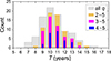 |
Fig. 7. Histogram of the solar cycle lengths (T; min-to-min) for all the reconstructed cycles (grey shaded bars) and for cycles corresponding to different values of the quality flag (q), as indicated in the legend. |
The validity of empirical relations, including the Waldmeier rule, remains inconclusive for the reconstructed cycles, likely due to uncertainties in the cycle shape.
5. Conclusions
An annual reconstruction of solar activity in the form of the SN (in the ISN v.2 definition) is presented for the first millennium CE, viz. 1–969 CE. The reconstruction is based on the annual measurements of Δ14C by Wang et al. (2026), involves an MCMC reconstruction method (Usoskin et al. 2021, 2025), and accounts for different sources of uncertainties in a straightforward manner. The reconstructed series covers one grand solar minimum, called the Horrebow minimum, from the period 650–730 CE, which is comparable to the Maunder minimum. There are a few shorter episodes of low activity occurring circa 120, 250, and 900 CE, resembling the Dalton minimum, which is usually not considered a grand minimum (Schüssler et al. 1997; Usoskin 2023). The time-frequency analysis, based on the wavelet spectrum, shows that the only significant quasi-periodicity in the reconstructed series is related to the Schwabe cycle. Other periodicities, such as the Suess or de Vries cycles and the Gleissberg variability or its harmonics, appear insignificant. There was a strong ESPE in 774 CE, the strongest one known during the Holocene. The data were corrected for it, but reconstructed cycles 73–75 may well still be affected by the event.
Based on this SN reconstruction, we identified 91 solar cycles during that period, of which 26 are well defined (q ≥ 4), 24 are reasonably well defined (q = 3), 31 are poorly defined (q = 1–2), and 10 can only be guessed. This dataset provides no conclusive evidence for the existence of Waldmeier’s relations.
The results of this work fill the gap in the solar cycle statistics between the first millennium BCE (Brehm et al. 2021; Usoskin et al. 2021) and the second millennium CE (Brehm et al. 2025; Usoskin et al. 2025). The total number of resolved solar cycles is now about 280, which is much greater than the 25 directly observed cycles in the ISN data series (Clette & Lefèvre 2016). This provides greatly improved statistical constraints on solar dynamo theory as well as on the models of solar irradiance on the millennial timescale. However, two caveats should be considered: (1) Many of the reconstructed cycles are rather uncertain. If only the reliably reconstructed cycles are considered, i.e. those with q ≥ 4, 74 cycles can be identified. This, however, is still three times more than the directly measured ones. (2) This collective statistic is based on three stand-alone pieces of millennium-long reconstructions with possible boundary distortions between them. A consistent 3-millennium-long reconstruction of SNs, based on a composite multi-proxy cosmogenic record, is pending.
Data availability
The table containing the reconstructed sunspot values with uncertainties is available at the CDS via https://cdsarc.cds.unistra.fr/viz-bin/cat/J/A+A/708/A333
Acknowledgments
This work has received funding from the European Research Council for a Synergy Grant (project 101166910) and an Advanced Grant (grant agreement No. 101097844 – project WINSUN), as well as from the Research Council of Finland (Space Resilience Centre of Excellence, project 374100).
References
- Beer, J., McCracken, K., & von Steiger, R. 2012, Cosmogenic Radionuclides: Theory and Applications in the Terrestrial and Space Environments (Berlin: Springer) [Google Scholar]
- Biswas, A., Karak, B., Usoskin, I., & Weisshaar, E. 2023, Space SCi. Rev., 219, 19 [Google Scholar]
- Brehm, N., Bayliss, A., Christl, M., et al. 2021, Nat. Geosci., 14, 10 [Google Scholar]
- Brehm, N., Pearson, C., Christl, M., et al. 2025, Nat. Comm., 16, 406 [Google Scholar]
- Büntgen, U., Wacker, L., Galvan, J., et al. 2018, Nat. Comm., 9, 3605 [Google Scholar]
- Charbonneau, P. 2020, Liv. Rev. Sol. Phys., 17, 4 [Google Scholar]
- Clette, F., & Lefèvre, L. 2016, Sol. Phys., 291, 2629 [Google Scholar]
- Cliver, E. W., Schrijver, C. J., Shibata, K., & Usoskin, I. G. 2022, Liv. Rev. Sol. Phys., 19, 2 [NASA ADS] [CrossRef] [Google Scholar]
- Eddy, J. 1976, Science, 192, 1189 [Google Scholar]
- Golubenko, K., Usoskin, I., Rozanov, E., & Bard, E. 2025, Earth Planet. Sci. Lett., 661, 119383 [Google Scholar]
- Gray, L. J., Beer, J., Geller, M., et al. 2010, Rev. Geophys., 48, RG4001 [Google Scholar]
- Güttler, D., Adolphi, F., Beer, J., et al. 2015, Earth Planet. Sci. Lett., 411, 290 [Google Scholar]
- Haigh, J. D., Winning, A. R., Toumi, R., & Harder, J. W. 2010, Nature, 467, 696 [CrossRef] [Google Scholar]
- Hathaway, D. H. 2015, Liv. Rev. Sol. Phys., 12, 4 [Google Scholar]
- Heaton, T., Bard, E., Bayliss, A., et al. 2024, Nature, 633, 306 [Google Scholar]
- Herbst, K., Kopp, A., Heber, B., et al. 2010, J. Geophys. Res., 115, D00I20 [Google Scholar]
- Inceoglu, F., Simoniello, R., Knudsen, V. F., et al. 2015, A&A, 577, A20 [CrossRef] [EDP Sciences] [Google Scholar]
- Kaiser Kudsk, S., Knudsen, M., Karoff, C., et al. 2022, Quat. Sci. Rev., 292, 107617 [Google Scholar]
- Karak, B. 2023, Liv. Rev. Sol. Phys., 20, 3 [NASA ADS] [CrossRef] [Google Scholar]
- Knudsen, M. F., Riisager, P., Donadini, F., et al. 2008, Earth Planet. Sci. Lett., 272, 319 [CrossRef] [Google Scholar]
- Miyake, F., Nagaya, K., Masuda, K., & Nakamura, T. 2012, Nature, 486, 240 [NASA ADS] [CrossRef] [Google Scholar]
- Miyake, F., Usoskin, I., & Poluianov, S. 2020, Extreme Solar Particle Storms: The Hostile Sun (Bristol, UK: IOP Publishing) [Google Scholar]
- Nilsson, A., Suttie, N., Stoner, J., & Muscheler, R. 2022, Proc. Natl. Acad. Sci., 119, e2200749119 [Google Scholar]
- Panovska, S., Poluianov, S., Gao, J., et al. 2023, J. Geophys. Res. (Space Phys.), 128, e2022JA031158 [Google Scholar]
- Pavón-Carrasco, F. J., Osete, M. L., Torta, J. M., & De Santis, A. 2014, Earth Planet. Sci. Lett., 388, 98 [Google Scholar]
- Schanner, M., Korte, M., & Holschneider, M. 2022, J. Geophys. Res. (Solid Earth), 127, e2021JB023166 [Google Scholar]
- Schüssler, M., Schmitt, D., & Ferriz-Mas, A. 1997, ASP Conf. Ser., 118, 39 [Google Scholar]
- Solanki, S. K., Usoskin, I. G., Kromer, B., Schüssler, M., & Beer, J. 2004, Nature, 431, 1084 [Google Scholar]
- Steinhilber, F., Abreu, J., Beer, J., et al. 2012, Proc. Natl. Acad. Sci., 109, 5967 [Google Scholar]
- Usoskin, I. G. 2023, Liv. Rev. Sol. Phys., 20, 2 [NASA ADS] [CrossRef] [Google Scholar]
- Usoskin, I. G., Alanko-Huotari, K., Kovaltsov, G. A., & Mursula, K. 2005, J. Geophys. Res., 110, A12108 [Google Scholar]
- Usoskin, I. G., Solanki, S. K., Schüssler, M., Mursula, K., & Alanko, K. 2003, Phys. Rev. Lett., 91, 211101 [Google Scholar]
- Usoskin, I. G., Solanki, S. K., & Kovaltsov, G. A. 2007, A&A, 471, 301 [CrossRef] [EDP Sciences] [Google Scholar]
- Usoskin, I. G., Kromer, B., Ludlow, F., et al. 2013, A&A, 552, L3 [NASA ADS] [CrossRef] [EDP Sciences] [Google Scholar]
- Usoskin, I. G., Arlt, R., Asvestari, E., et al. 2015, A&A, 581, A95 [CrossRef] [EDP Sciences] [Google Scholar]
- Usoskin, I. G., Gallet, Y., Lopes, F., Kovaltsov, G. A., & Hulot, G. 2016, A&A, 587, A150 [CrossRef] [EDP Sciences] [Google Scholar]
- Usoskin, I. G., Solanki, S. K., Krivova, N., et al. 2021, A&A, 649, A141 [EDP Sciences] [Google Scholar]
- Usoskin, I., Chatzistergos, T., Solanki, S. K., et al. 2025, A&A, 698, A182 [NASA ADS] [CrossRef] [EDP Sciences] [Google Scholar]
- Vaquero, J. M., Kovaltsov, G. A., Usoskin, I. G., Carrasco, V. M. S., & Gallego, M. C. 2015, A&A, 577, A71 [CrossRef] [EDP Sciences] [Google Scholar]
- Vonmoos, M., Beer, J., & Muscheler, R. 2006, J. Geophys. Res., 111, A10105 [Google Scholar]
- Waldmeier, M. 1939, Astron. Mitt. Zurich, 14, 470 [NASA ADS] [Google Scholar]
- Wang, J., Dee, M. W., Pope, B. J. S., et al. 2026, Commun. Earth Environ., 7, 96 [Google Scholar]
- Wu, C. J., Usoskin, I. G., Krivova, N., et al. 2018, A&A, 615, A93 [NASA ADS] [CrossRef] [EDP Sciences] [Google Scholar]
Appendix A: Reconstructed solar cycles
Reconstructed solar cycles and their parameters.
All Tables
All Figures
|
Fig. 1. Sequential steps of the annual solar activity reconstructions for the first millennium CE. Panel (a): raw Δ14C data (Wang et al. 2026). The red arrow indicates the signature of the ESPE of 774 CE. Panel (b): 14C production rate (Q*) corrected for geomagnetic shielding and ESPE effects. Panel (c): OSF (Fo). Panel (d): SN. Black curves, grey shading, and red curves depict the annual values, 1σ (68% confidence interval) uncertainties, and 22-year smoothed data, respectively. |
| In the text | |
|
Fig. 2. Recent reconstructions of the geomagnetic VDM for the first millennium CE. The models are P23 (Panovska et al. 2023), K08 (Knudsen et al. 2008), PAV14 (Pavón-Carrasco et al. 2014), N22 (Nilsson et al. 2022), U16 (Usoskin et al. 2016), and AK (Schanner et al. 2022). |
| In the text | |
|
Fig. 3. Correction of the dataset for the ESPE of 774 CE. Panel (a): mean raw Δ14C annual data (black curve), the modelled 774 response (dashed blue lines; T = 130 DoY, A = 3.5; see Golubenko et al. 2025), and de-trended Δ14C data (dash-dotted red curve). Panel (b): SNs reconstructed from the raw Δ14C (black) and de-trended (red) datasets. Error bars are omitted for clarity in all panels. |
| In the text | |
|
Fig. 4. Different sources of uncertainties of the SN reconstruction plotted at the 1σ level: radiocarbon measurement errors (red Δ14C line), geomagnetic models (blue VDM line), model uncertainties (magenta line) including both the computation of the OSF and the OSF-to-SSN conversion, and the total uncertainty (green line), which is close to the geometrical sum of the individual uncertainties. The dashed black line represents the diagonal. |
| In the text | |
|
Fig. 5. SNs (ISN_v2 normalisation) reconstructed here for 1–969 CE, split into two panels for clarity. The black curve, grey shading, and red curve depict the mean annual reconstructed SN, its 68% confidence interval, and the 22-year smoothed evolution (see main text), respectively. These data are identical to those in Fig. 1d. The digital version of these data is available at the CDS. The green curve depicts the smooth decadal SN values reconstructed from multi-proxy cosmogenic isotope data (Wu et al. 2018). |
| In the text | |
|
Fig. 6. Wavelet spectrum (Morlet basis, k = 6) of the reconstructed annual mean SN series. The black-contoured areas represent the statistically significant spectral power (p < 0.05 against the AR1 red noise). The white line bounds the cone of influence, below which the results are unreliable. |
| In the text | |
|
Fig. 7. Histogram of the solar cycle lengths (T; min-to-min) for all the reconstructed cycles (grey shaded bars) and for cycles corresponding to different values of the quality flag (q), as indicated in the legend. |
| In the text | |
Current usage metrics show cumulative count of Article Views (full-text article views including HTML views, PDF and ePub downloads, according to the available data) and Abstracts Views on Vision4Press platform.
Data correspond to usage on the plateform after 2015. The current usage metrics is available 48-96 hours after online publication and is updated daily on week days.
Initial download of the metrics may take a while.