| Issue |
A&A
Volume 708, April 2026
|
|
|---|---|---|
| Article Number | A354 | |
| Number of page(s) | 14 | |
| Section | Celestial mechanics and astrometry | |
| DOI | https://doi.org/10.1051/0004-6361/202558833 | |
| Published online | 24 April 2026 | |
Two-stage formation of the Moon from accreting fragmentation and resonance captures
1
Observatoire de Genève, Université de Genève,
Chemin Pegasi, 51,
1290
Versoix,
Switzerland
2
LTE, Obs. de Paris, Univ. PSL, Sorbonne Univ., Univ. de Lille,
LNE, CNRS, 61 Av. de l’Observatoire,
75014
Paris,
France
3
Dept. of Physics and Astronomy, University of Rochester,
Bausch & Lomb Hall,
Rochester,
NY
14627,
USA
4
Dept. of Earth and Environmental Siences, University of Rochester,
227 Hutchison Hall,
Rochester,
NY
14627,
USA
★ Corresponding author: This email address is being protected from spambots. You need JavaScript enabled to view it.
Received:
31
December
2025
Accepted:
27
February
2026
Abstract
Context. In the canonical Moon-forming model, a Mars-sized object collided with Earth to produce a disk of debris from which the Moon is believed to have accreted.
Aims. In order to build on past works, we simulated disks containing up to 105 debris (called moonlets) and we took fragmentation of the debris into account in the case of violent collisions.
Methods. We used the new software NcorpiON, and in particular its module FalcON, for fast gravity computation using multipole expansions. The built-in fragmentation model of NcorpiON was used to resolve collisions. The initial conditions of our N-body simulations were output of smoothed particle hydrodynamic (SPH) simulations.
Results. Unlike previous works, we find that the Moon probably did not form in one step but rather in two stages. The first stage lasts a few months to a few tens of years and is dominated by collisions and gravitational scattering. It often leads to several large submoons. In the second stage, of length 103 to 105 years, tidal forces and subsequent migration allow these submoons to be captured in mean motion resonances (MMR), cleaning the system and completing the formation of the Moon through ejections and collisions.
Conclusions. A significant mass is lost during the accretion process, and we favor protolunar disks with initially at least 2M☾.
Key words: celestial mechanics / Earth / Moon / planets and satellites: formation
© The Authors 2026
 Open Access article, published by EDP Sciences, under the terms of the Creative Commons Attribution License (https://creativecommons.org/licenses/by/4.0), which permits unrestricted use, distribution, and reproduction in any medium, provided the original work is properly cited.
This article is published in open access under the Subscribe to Open model. This email address is being protected from spambots. You need JavaScript enabled to view it. to support open access publication.
1 Introduction
It is accepted that the Moon formed from a disk following an impact between the proto-Earth and an impactor dubbed Theia (Hartmann & Davis 1975; Cameron & Ward 1976). In the so-called canonical model, Theia is a Mars-sized object (Canup & Asphaug 2001). This model can explain several features of the Earth-Moon system, such as the mass of the Moon, the angular momentum of the Earth-Moon system, or the size of the lunar core, but the details, including the velocity of the impactor or its size, are not well understood. Furthermore, the canonical model tends to produce a disk mostly made of impactor material, making it hard to reconcile this model with the observation that the Moon and Earth share similar isotopic ratios (e.g., Zhang et al. 2012; Canup et al. 2023; Sossi et al. 2024). In order to address this issue, more recent models propose different hypotheses, namely:
Multiple impact model (Rufu et al. 2017): small impacts form small submoons which eventually merge.
Synestia model (Cuk & Stewart 2012; Lock et al. 2018): a high angular momentum and high energy impact forms a gaseous or supercritical disk from which the Moon condensates.
Half-Earths model (Canup 2012): the Moon forms from the disk subsequent to a collision between two half-Earth-sized objects.
Among the differences in these models, the kinetic energy involved in an impact is much larger in the synestia and halfEarth models than in the canonical and multiple impact models. As a result, these energetic models nearly or completely produce vapor disks, which may constitute a challenge, as moonlets face strong gas drag and fall onto Earth before they can grow and become large (Nakajima et al. 2022, 2024).
Another major issue is the angular momentum of the Earth-Moon system after the impact. In the canonical model, the angular momentum is similar to the current value, but in the energetic models, it is two to three times higher, and this excess needs to be removed to match the current value. Cuk & Stewart (2012) suggested that a capture in the evection resonance can remove this excess, by transferring angular momentum from the Earth-Moon system to the Sun-Earth orbit, but such capture requires slow enough tidal migration (Touma & Wisdom 1998). Furthermore, Ward et al. (2020) and Rufu & Canup (2020) find that even in the case of capture in the evection resonance, the angular momentum loss is marginal.
Previous numerical works on the formation of the Moon considered disks such that (e.g., Ida et al. 1997; Salmon & Canup 2012):
Moonlets were initially randomly generated around the proto-Earth.
The total number of moonlets was typically ≲103.
Collisions were resolved by either a merger or a bounce depending on rebound velocity.
The initial disk structure can potentially affect how the Moon formed. For this work, we built upon previous works by improving these points. We investigated the Moon formation process starting shortly after the impact using both the results of smoothed particle hydrodynamic (SPH) simulations and randomly generated disks as initial conditions. We resolved collisions with the assumptions that moonlets can fragment. Our debris disks contained up to 105 moonlets.
In Sect. 2, we explain the assumptions of our model, the physical contributions taken into account, and the initial conditions used to carry out the numerical simulations. In Sect. 3, we describe the two formation stages that the Moon probably went through, and we explain why our simulations can only be considered as possible formation scenarios. In Sect. 4, we present the final states of our simulations before discussing them in Sect. 5. Finally, we draw conclusions and explore future directions in Sect. 6. For convenience to the reader, in Table A.1 of Appendix A, we provide all of the notations used throughout this work. We only briefly mention the evection resonance is this work, but a follow-up paper will be entirely dedicated to it.
2 Model
The outcome of the simulation of a protolunar disk depends on the physical contributions that are considered, the initial conditions and the numerical precision. In this section, we detail our Moon-forming model. Hereafter, O denotes the center of mass of the system, and in a general fashion, the mass and radius of Earth are denoted by M⊕ and R⊕, while the mass of the Moon is denoted M☾. Let N be the total number of bodies orbiting Earth and for 1 ≤ j ≤ N, mj is the mass of the jth body. The inertial reference frame is (O, i, j, k), while the reference frame attached to the rotation of Earth is (O, I, J, K), with k = K. The transformation from one to another is done through application of the rotation matrix Ω, which is the sidereal rotation of Earth. All vectors and tensors of this work are bolded, whereas their norms, as well as scalar quantities in general, are unbolded. We also denote uj the position of the jth body in the inertial reference frame, and u⊕ the position of Earth in that same reference frame.
2.1 N-body simulations
Our simulations were carried out on the new software NcorpiON1 (Couturier et al. 2025), that we improved so it can handle all the physical contributions discussed below. We ran N-body simulations, where the debris coming from the giant impact between Earth and Theia were assumed to be spherical individual bodies called moonlets.
We denote  the orbital period of a massless particle with semi-major axis 1R⊕. NcorpiON works in a system of units where Ms = R⊕ = T⊕ = 1 (We take G = 4π2 for the gravitational constant). The conversion back to SI units is done via:
M⊕ = 5.972 × 1024 kg
R⊕ = 6371 km
T⊕ = 5061 s
We used a timestep dτ = 2−6 T⊕ ≈ 79 seconds in our simulations.
2.1.1 Gravitational forces
The first contribution to be taken into account is gravity. In our model, moonlets interact gravitationally with Earth, with each other, and with the Sun. We describe in Sect. 2.2 how we guaranteed a fast computation of the mutual gravity.
Since the moonlets are assumed spherical and homogeneous, the gravity between them can be computed as if they were pointmass. However, Earth was spinning fast at the time of the Moon formation, with a length of day in the range [2.5,6] hours. Such a fast rotation rate means that Earth had a significant equatorial bulge, that we took into account by means of the second zonal harmonic J2. More precisely, the acceleration of moonlet j due to its interaction with Earth reads (Couturier et al. 2025, Eq. (B.14))
![Mathematical equation: \ddot{\vect{u}}_j=-\frac{\G\Mearth\vect{r}_j}{r_j^3}+\frac{\G\Mearth\Rearth^2J_2}{r_j^5}\left[\frac{15z_j^2-3r_j^2}{2r_j^2}\vect{r}_j-3z_j\vect{k}\right]\!,\!](/articles/aa/full_html/2026/04/aa58833-25/aa58833-25-eq2.png) (1)
(1)
where rj = uj - u⊕ = xji + yjj + Zjk. By conservation of the total momentum, the acceleration of Earth is then  . Assuming that Earth was fluid and molten after the giant impact, the second zonal harmonic is related to the rotation rate Ω of Earth by (Wahr 1996, Sect. 4.2.1)
 (2)
(2)
In NcorpiON, we set the six elliptic elements of the Sun-Earth orbit to correspond to a circular orbit of semi-major axis 23 481R⊕ = 1 AU. Since impacts formed Earth isotropically (e.g., Kokubo & Ida 2000), we do not know the obliquity of Earth at the time of Theia impact, nor how Theia affected Earth’s obliquity. In our simulations, we arbitrarily set the Sun-Earth orbit to be in Earth’s equatorial plane (zero obliquity).
2.1.2 Roche radius and tidal disruption
Besides the spherical assumption, we also considered that the moonlets have no internal cohesion. At the beginning of the simulation, this is because they were hot and molten, whereas near the end of the simulation, this is because the few remaining submoons were large enough to be at hydrostatic equilibrium. This absence of internal cohesion means that moonlets orbiting Earth below the Roche radius are disrupted by tidal forces. For a moonlet with lunar density on a circular orbit, the Roche radius is located at 2.9R⊕. Moonlets on eccentric trajectories can get closer than that (Nduka 1971), and for our simulations, we set the disruption threshold in NcorpiON to be 1.8 R⊕, so moonlets spawning from the inner fluid disk are not disrupted right away.
Tidally disrupted moonlets form an inner fluid disk. We implemented an inner fluid disk in NcorpiON following the model of Salmon & Canup (2012) and made the new version available on the github repository. Whenever a moonlet plunged below the Roche radius, it was removed from the N-body code and its mass added to the inner fluid disk. The inner fluid disk was homogeneous (disk density was a function of time only) and lied on the equatorial plane between 1R⊕ and a variable outer edge Rout. Because of viscous spreading, mass flowed from the inner and outer edges of the disk at rates (Salmon & Canup 2012, Appendix A)
 (3)
(3)
where  is the viscosity of the disk, ω2(r) = GM⊙/r3, Σf is the disk mass per unit area, x = Rout/R⊕ and f(x) is given by Eq. (A5) of Salmon & Canup (2012). The flow out of the outer edge allowed moonlets of typical mass (Goldreich & Ward 1973)
 (4)
(4)
to spawn from the outer edge of the disk with a typical frequency  . In this expression, f̃ is a dimensionless parameter that Salmon & Canup (2012) take to be 0.3. We adopted the same choice. Every ∆̃t, the mass mspw was removed from the inner fluid disk and a moonlet of same mass was spawned on a circular and equatorial orbit with semi-major axis Rout. The mass flowing out of the fluid disk by the inner edge was removed from the disk and added to Earth. We neglected tidal interactions between the inner fluid disk and the moonlets in our work, as well as spiral density waves in the inner fluid disk.
In Salmon & Canup (2012), whenever a moonlet approaches Earth closer than the disruption threshold, it is removed from the N-body simulation and its mass added to the inner fluid disk. However, this does not account for the possibility that the disrupted moonlet could fall directly onto Earth. In NcorpiON, we added the mass of the disrupted moonlet to the fluid disk only if either of these conditions was met
The periapsis of the moonlet is above the surface, or
The periapsis is below the surface, but the moonlet crosses the equatorial plane before hitting the surface.
The first condition translates into a (1 - e) > R⊕, where a is the semi-major axis and e the eccentricity, whereas the second condition translates into zẑ < 0, where z is the z-coordinate of the moonlet in the geocentric frame when it crosses the disruption threshold, and ẑ is the z-coordinate of the hitting point, in the same reference frame. If none of these two conditions was met, then the mass of the disrupted moonlet was added to Earth.
When a moonlet spawned from or merged with the inner fluid disk, the outer edge Rout was updated to conserve the total angular momentum. For simplicity, we assumed that the inner fluid disk remained on the equatorial plane and only the z-component of the total angular momentum was conserved.
2.1.3 Tidal model
Since Earth is an extended body, moonlets are able to raise tidal bulges on it, which modifies the distribution of mass within Earth. This redistribution of mass changes Earth’s gravity field and the orbits of the moonlets are subsequently affected. While tidal forces can be disregarded on short timescales, they become important on longer timescales because of drifts in semi-major axes. As we see in Sect. 3.4, these drifts are important, which is why we considered tides in our simulations.
We implemented the constant timelag model in NcorpiON (Singer 1968; Mignard 1979), that we describe here in a modern way. Let rk be the position of the kth moonlet with respect to Earth center in the frame (O, I, J, K) attached to Earth’s rotation and r a point within Earth in the same reference frame. The moonlet raises at r the potential
 (5)
(5)
called perturbing potential. In this expression, the Pl are the Legendre polynomials. Terms l ≤ 1 have a gradient independent on r. Since tides come from a differential acceleration within Earth, these terms do not contribute to tides and are discarded. Terms l ≥ 3 are also discarded due to the small size of r/rk. Using P2(z) = (3z2 - 1)/2, the perturbing potential is rewritten
 (6)
(6)
The perturbing potential W governs how moonlet k redistributes mass in Earth. The redistribution of mass raises a potential V, called perturbed potential. Moonlet k itself or another moonlet at position rj feels the potential V and is affected by tides. The challenge in tidal theories is to relate the perturbed potential V to the perturbing potential W. Assuming these three hypothesis:
- (i)
The tidal perturbations are small enough so that V depends linearly on W,
- (ii)
The geophysical properties of Earth are constant over the tidal timescales,
- (iii)
Earth is isotropic in the absence of tides2,
it can be shown (Boué et al. 2019; Couturier 2022) that, at the quadrupolar order, V is related to W by the convolution product
 (7)
(7)
where k2(t) is the second Love distribution of Earth and characterizes its memory of past stresses. In order to get rid of the convolution product, a common choice is the constant-∆t model where k2 is taken proportional to a Dirac distribution
 (8)
(8)
In this expression, the second Love number κ2 measures the ability of Earth to get deformed by tides and the timelag ∆t measures its ability to dissipate energy when it is deformed by tides. Injecting Eqs. (6) and (8) into Eq. (7), we obtain for the perturbed potential felt by the moonlet at position rj
![Mathematical equation: V(\vect{r}_j)=-\frac{1}{2}\kappa_2\frac{\G m_k \Rearth^5}{r_j^5r_k^{\star5}}\left[3\left(\vect{r}_j\cdot\vect{r}_k^\star\right)^2-r_j^2r_k^{\star2}\right],](/articles/aa/full_html/2026/04/aa58833-25/aa58833-25-eq13.png) (9)
(9)
where, in the rotating frame,  . The perturbed potential is currently written in the frame attached to Earth’s rotation. We switch to the inertial reference frame (O, i, j, k) by application of the rotation around the vector Ω, which is the sidereal rotation of Earth. Because V depends on rj and
  only through their norm and through their scalar product, its expression is unaffected by the rotation and is still given by Eq. (9). Only the expression of
  is affected. Provided that the timelag ∆t is small with respect to the moonlets’ orbital period and the length of day, we have, in the inertial frame
 (10)
(10)
We keep the same notations for rj and rk despite the change of reference frame. A moonlet can feel the perturbed potential caused by itself (j = k) or by another moonlet (j ≠ k). However, when two moonlets are not in a mean motion resonance (MMR), the perturbed potential with j ≠ k averages out. Therefore, we consider for the tidal model of NcorpiON that moonlets only feel their own tide. When moonlets are captured in a MMR, our tidal model fails, but tides are unimportant compared to moonlet-moonlet interactions in this case. When the MMR is broken (by ejection or collision), the tidal model becomes valid again. Differentiating Eq. (9) with respect to rj, specializing to j = k and expanding to first order in ∆t yields the tidal acceleration (Mignard 1979, Eq. (5))
![Mathematical equation: \ddot{\vect{r}}_j\!=\!-3\kappa_2\G m_j\frac{\Rearth^5}{r_j^{10}}\left[r_j^2\vect{r}_j\!+\!\Delta t\left(2\left(\vect{r}_j\cdot\vect{v}_j\right)\vect{r}_j\!+\!r_j^2\left(\vect{v}_j\!+\!\vect{r}_j\times\vect{\Omega}\right)\right)\right]\!,](/articles/aa/full_html/2026/04/aa58833-25/aa58833-25-eq18.png) (11)
(11)
where  . Tides cause an exchange of angular momentum between the orbits and Earth’s rotation. To conserve the angular momentum, we updated Earth’s rotation with
 (12)
(12)
where I⊕ is the inertia matrix of Earth and  is given by Eq. (11). For simplicity and to prevent a departure from shortest axis rotation, we considered that Ω = Ωk at all time and we only verified the third coordinate of Eq. (12)
 (13)
(13)
where C⊕ is Earth’s largest moment of inertia. Equation (13) predicts a variation of the rotation rate and subsequently of the second zonal harmonics J2 according to Eq. (2).
We set the second Love number κ2 to 3/2 in NcorpiON, valid for a fluid and molten Earth (Roberts & Nimmo 2008). Estimating a correct value for ∆t is not simple. The current value is ∆t ~ 638 s (Q ~ 11), but Touma & Wisdom (1998) justify that ∆t was at least 25 times smaller at the time of the Moon formation, which gives an upper bound ∆t ≤ 25 s. Using typical frequencies, the work of Zahnle et al. (2015) further constrain ∆t ≤ 1 s from their estimate of the quality factor. Despite this last estimate, we adopted ∆t = 8 s in our simulations to prevent them from being too long. This could lead us to underestimate by a factor at least 8 the length of the second stage of the Moon formation (Sect. 3.4). It is possible that very weak secular resonances that would have led to minor dynamical instabilities with ∆t ≤ 1 s are avoided with this higher value, but strong resonances such as first-order MMR that mainly shape the dynamics are not evaded by this choice.
2.2 Mutual gravity with FalcON
At each timestep, the moonlets’ gravitational interactions with Earth and with the Sun are handled in O(N) time via a direct summation. However, computing the mutual gravity between the moonlets via a direct summation requires O(N2) force calculations, which effectively limits the maximal value of N to a few thousands (max 2000 in Salmon & Canup 2012). This is incompatible with our use of the fragmentation model of NcorpiON (see Sect. 2.4), where N can exceed ∼ 105 in our simulations.
Therefore, we computed mutual gravity between the moon-lets using the fast multipole method FalcON (Dehnen 2002, 2014). FalcON is an improvement over the standard tree code of Barnes & Hut (1986) and works by computing multipole moments between cells in an octree. It is ∼20 times faster than REBOUND’s tree code for the same precision (Couturier et al. 2025, Fig. 6) and vastly faster than a direct summation for large N. NcorpiON comes with its own implementation of FalcON, that we used for our project.
The gain of time comes at the cost of a precision loss that can be controlled through the order p or the multipole expansions and the opening angle3 θ of the octree cells, derived from the opening angle θmin of the root cell via Eq. (13) of Dehnen (2002). Both p and θmin are parameters of NcorpiON. For our simulations, we set p = 3 and θmin = 0.45, which resulted in a median relative error in the force calculation ∼0.0038% and a relative error at the 99th percentile ∼0.042% (using Table D.3 of Couturier et al. 2025, considering a ratio ∼39 in Earth to disk mass). For N = 105, we were able to compute five timesteps per second versus one timestep per minute with the brute-force method. For N = 110, a direct summation is equally as fast as FalcON, and in the late stages of the simulations, when N ≤ 110 (see Fig. 4), we switched to the brute force method.
Due to the highly chaotic nature of the simulated systems (see Sect. 3.1), these small errors affect the outcome of a given simulation. However, since they are analogous to a slight change in initial conditions (it is as if a new simulations starting from that new timestep had its initial conditions slightly changed), they do not change the statistical behavior of the simulations.
Four sets of initial conditions of this work.
2.3 Initial conditions
We present in this work four simulations from a set of four different initial conditions given in Table 1.
The outcome of a simulation depends as much on the choice of initial conditions than on the differential system implemented. Therefore, in order to limit the amount of arbitrary decisions in our work, three of these initial conditions were extracted from SPH simulations of the giant impact between the proto-Earth and Theia (canonical model) or between two half Earths (halfEarth model). Only one set of initial conditions corresponds to a randomly generated protolunar disk.
Two of these initial conditions, called “500b073S” and “500b075S”, represent canonical Moon-forming impacts. These datasets are outputs at time t = 40 hours after impact of SPH simulations conducted by Hull et al. (2024). The prefix 500 in the name refers to the cut-off density in kg/m3, the substrings b073 and b075 refer to the normalized impact parameter between Theia and the proto-Earth, and the suffix S indicates the equation of state used in their work. We refer the reader to Table 1 of Hull et al. (2024) for more details and explanations.
Another initial condition, called “half-Earth” represents the half-Earths model and corresponds to time t = 69.445 hours after impact of the simulation mentioned in Table 2 of Hull et al. (2026). The last set of initial conditions, called “random”, is a randomly generated disk with 104 moonlets around Earth. We arbitrarily set its initial time to 40 hours. The moonlets’ initial elliptic elements4 were drawn uniformly at random in the ranges (a, e, i; ν, ω, Ω) ∊ ([2.9,25] R⊕, [0,0.2], [0, 8°]; [0,2π]3). Their densities were chosen uniformly at random in the range [0.1048,0.1848] M⊕/R3⊕ (The Moon’s density is 0.1448M⊕/R3⊕ = 3344 kg/m3). Finally, their radii were chosen uniformly in the range [0.002, 0.0225] R⊕.
The SPH simulations “500b073S” and “500b075S” used N = 1 149 900 particles, whereas “half-Earth” used N = 2 001000 particles. However, most of these particles were part of Earth which is one single extended body. To discriminate between particles of Earth and particles of the disk, we first identified the center of Earth by locating the center of mass of particles labeled “target core” in the SPH output. Then, going outward from that point, the density of particles suddenly drops at a certain radius, and all particles below (resp. beyond) that radius were said to belong to Earth (resp. to the disk). In the disk, some particles were clumped together and we considered them as a single moonlet. Particles of the disk that were not part of a clump were taken as one moonlet. These moonlets have a mass 0.886 10−6 Mæ for the canonical initial conditions and either 0.495 10−6 M⊕ or 0.605 10−6 M⊕ for the half-Earth initial conditions, which is the mass of a SPH particle and the minimal mass at initial time. The initial number N0 of moonlets in our N-body simulations is indicated in Table 1. The SPH output does not constrain the radii but only the masses. The radii were obtained by giving density 0.1448 M⊕/R3⊕ = 3344 kg/m3 to all moonlets. Finally, the initial sidereal rotation of Earth was obtained from the velocities of particles of Earth. At the beginning of the simulations, the inner fluid disk was filled with moonlets that were below the Roche radius. In Fig. 1, we show a 3D representation of these initial conditions5.
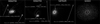 |
Fig. 1 3D visualization of the initial conditions. Moonlets are displayed six times bigger than they actually are, whereas Earth is displayed with its true radius and indicates the scale. The red cross is the center of mass of the system and is inside Earth. The masses and orbital elements of notable moonlets are indicated. Some have highly eccentric orbits and are quickly lost. |
2.4 Collisions and fragmentation
A difficulty in N-body disk simulations lies in the search and resolution of collisions. As for mutual gravity computation, a bruteforce collision search yields a O(N2) method, and NcorpiON adapts FalcON to rapidly locate collisions (Couturier et al. 2025). Once collisions are detected, their resolution influences the degree of realism of the simulation. Previous works resolve collisions from inelastic rebounds, and the relative velocity after impact determines if the colliding particles should be merged or not (Ida et al. 1997; Kokubo et al. 2000; Salmon & Canup 2012). However, the possible fragmentation of moonlets following a violent collision has not yet been considered in an N-body Moon-forming simulation.
Although Kokubo et al. (2000) argue that fragmentations should not play an important role because they do not change the overall disk density, we prefer to take fragmentations into account in our model as they hinder accretion, which is an essential aspect of the Moon formation. Our fragmentation model is the one described in Couturier et al. (2025), that relies on the works of Housen & Holsapple (2011) for crater scaling and ejecta models, Leinhardt & Stewart (2012) for fragment sizes and super-catastrophic collisions, and Suetsugu et al. (2018) for dependency on impact angles. While we do not delve deeply into the model here (we refer the reader to Sect. 5.3. of Couturier et al. 2025, for details), we shall recall that when a collision between two moonlets of masses m1 and m2 occurs, we write
 (14)
(14)
where m̃ is the mass of the largest remnant and m̌ is the mass of the debris tail, defined as the set of fragments unbounded to the largest remnant. Some parameters of NcorpiON are decision thresholds about the values of m̃ and m̌ that we set in this way:
If m̌ < 0.0002 (m1 + m2), the colliding moonlets are merged.
If m̌ ≥ 2.25 × 10⁻⁷M⊕ or if m̌ > m̃, then the tail is divided into 15 moonlets whose mass distribution is given by Leinhardt & Stewart (2012) and speed distribution by Housen & Holsapple (2011). See (Couturier et al. 2025, Sect. 5.3.5) for details. Otherwise, the tail is reunited into one single moonlet.
If m̃ < (m1 + m2)/10 (super-catastrophic collision), then the tail is too fragmented to be handled with individual moon-lets. We discard it from the simulation but its mass is added to the inner fluid disk for conservation. The largest remnant is kept in the simulation.
These thresholds are a compromise between the degree of realism and keeping the total number N of moonlet reasonable. They are parameters of NcorpiON. Due to the assumptions made to its elaboration, the realism of NcorpiON’s fragmentation model could be altered when the colliding moonlet are roughly of the same mass, but we still expect it to be superior to a simple merging criterion based on rebound velocity. Super-catastrophic collisions produce arbitrarily small moonlets when m̃ ≪ m1 + m2. In order to prevent tiny moonlets from slowing down the simulation, the largest remnant of a super-catastrophic collision was removed from the N-body code and added to the inner fluid disk when m̃ < 5.625 × 10⁻⁸ M⊕.
3 Results
In this work, we only present in details four simulations, three starting from initial conditions obtained by previous SPH simulations, and one starting from a randomly generated disk. These four sets of initial conditions are presented in Table 1. Because of chaos, simulations with arbitrarily close initial conditions or parameters yield drastically different outcomes (e.g., Laskar & Gastineau 2009). Given the large amount of work associated with a statistical study, we decided to focus on four simulations that act as possible scenarios of Moon formation.
3.1 Chaos
In order to evaluate how chaotic the simulated systems are, we estimated their Lyapunov timescale by measuring the growth of initially close distances in the phase space. Starting from the initial condition “500b073S”, we first integrated for ten days to reach some arbitrary point in the phase space (called C0), with N ~ 18 000, that we used as starting point. From C0, we generated six very close initial conditions C1 to C6 by changing the positions of every moonlet by 10−11 R⊕ (∼6 μm) and the speeds by 10−11 R⊕/T⊕ (∼13 nm/s) in a random direction. From those points, we integrated the system for nine hours and we resolved collisions elastically in order to keep N constant. At each timestep, we measured the distance δ(t) in the phase space and position space between the two farthest simulations and fit it with
 (15)
(15)
Speeds and lengths were first both converted to km using R⊕ = T⊕ = 1 and the distance in the phase space between two points was then computed using the regular expression in Euclidean space. In Fig. 2, we show the distance δ(t) and the best exponential fit. Because no pair of the points C1 to C6 is separated by a vector collinear to the eigenmode associated with the largest Lyapunov exponent, the value of τ that we computed is not the Lyapunov time but only an estimate of it, that we call Lyapunov timescale. It should still give the order of magnitude of the Lyapunov time. We found a Lyapunov timescale
 (16)
(16)
showing that beyond a few hours and outside a statistical study, a Moon forming simulation can only be interpreted as a possible scenario, regardless on our confidence in the initial conditions.
3.2 Collisions and accretion
An interesting result that can be analyzed from a statistical point of view and should not be greatly affected by the chaotic nature of the system is how collisions distribute throughout the formation of the Moon. In particular, we are interested in how destructive or accreting collisions are, and we now define the catastrophicity C of a collision. A sensible definition is C = 1 - m̃/(m1 + m2) that yields a catastrophicity between 0 for a merger and 1 for a complete destruction. For visualization purposes though, it is better for the catastrophicity to take values in R+, and we define it instead as
![Mathematical equation: \mathcal{C}=\tan\left[\frac{\pi}{2}\left(1-\frac{\tilde{m}}{m_1+m_2}\right)\right].](/articles/aa/full_html/2026/04/aa58833-25/aa58833-25-eq26.png) (17)
(17)
With this definition, the catastrophicity of collisions assumed merged in our simulations is C ≈ 0.000314. Catastrophic collisions, defined as 2m̃ ≤ m1 + m2 (e.g., Benz & Asphaug 1999; Jutzi et al. 2009), correspond to C ≥ tan π/4 = 1. Finally, super-catastrophic collisions, defined as 10m̃ < m1 + m2, correspond to C ≳ 6.31, and are interesting in the sense that they are collisions for which m̃/(m1 + m2) is no longer proportional to the kinetic energy  of the collision but is instead proportional to
  (Stewart & Leinhardt 2009).
In Fig. 3, we show the distribution of catastrophicities of all the collisions that occurred in the 11 000 years of our simulations. The discontinuity at the threshold of super-catastrophicity is due to m̃ becoming proportional to  instead of QR. Indeed, as a result of this change of regime, we use Eq. (48) of Couturier et al. (2025) instead of Eq. (45) to compute m̃, and a collision is unlikely to be barely on the left of the threshold. A smoother change of regime, where the dependency progressively goes from m̃ × QR to
  would prevent the discontinuity.
Interestingly, some ∼30% of collisions were catastrophic, with about 25% being super-catastrophic. Some collisions even had catastrophicities C ≥ 50000, which corresponds to m̃ ≲ 10−5 (m1 + m2). This goes against Kokubo et al. (2000) argument that fragmentation of lunar seeds once formed outside the Roche radius is unlikely. Very disruptive collisions often happen when two small moonlets encounter. Indeed, their characteristic orbital speeds do not depend on their masses, but their mutual escape velocity does. Therefore, when two very small moon-lets collide, the ratio between their relative velocity and their escape velocity is generally high, resulting is a very disruptive collision. On the other side of the figure, collisions with catastrophicities C ≤ 10−8 generally occur when a very small moonlet collides with the largest moonlet. In that case, the large escape velocity coupled with the small mass m1 of the impactor does not allow for a disruptive collision. We concur with the remark of Kokubo et al. (2000) that since disruptive collisions involve small moonlets, whereas accreting collisions involve large ones, the formation of the Moon is not too much hindered by fragmentations. Disruptions of large moonlets occur as well, and taking fragmentations into account improves the model without being an absolutely necessary feature of a Moon forming model.
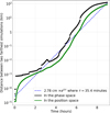 |
Fig. 2 Distance between the two farthest simulations in the phase space and in the position space and best exponential fit. The discontinuities in the black curve come from elastic collisions. The exponential fits the green curve. |
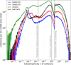 |
Fig. 3 Distribution of the catastrophicities of all collisions that occurred in our four runs. Run “500b073S”, “500b075S”, “half-Earth” and “random” had 163 202, 283 957, 539 143 and 1 000 405 collisions, respectively. Links to logs of all collisions for the four simulations are given in Table 4. |
3.3 First stage of the formation: Collisions
A generic scenario of formation breaks down into two stages where different mechanisms are involved. In the first stage, that lasts from soon after the giant impact to a few years after, collisions are numerous, and the subsequent accretion allows for typically one to three moonlets to grow significantly. During that time, fragmentations are first responsible for a quick increase in the number N of moonlets, before scattering allows most of the smallest moonlets to either escape the system or merge with either the inner fluid disk or a larger moonlet, making N decrease. In the second stage, most collisions involve a large submoons, and catastrophicities tend to be low, favoring mergers over disruptive collisions, and N keeps decreasing. However, this decrease is not monotonous, as N can sometimes temporarily grow back due to chain reactions of fragmentations, as can be seen from the spikes in Fig. 4, where we show the number N of moonlets and the frequency of collisions as a function of time.
Often enough, the first stage of the formation leads to the significant growth of more than one moonlet. Typically, a closein submoon emerges from material that spawned from the inner fluid disk, whereas another submoon comes from accretion at a larger distance from Earth. Cases where only one significant submoon emerges from the first stage are probably rare. These large submoons generally end up on well-separated orbits and do not collide during the first stage.
In Fig. 5, we plot the mass of the two most massive moonlets, of the inner fluid disk and the lost mass (mass fallen onto Earth or escaped) as a function of time for the four simulations. Escapes of large moonlets are visible through discontinuities in the green curve, while collisions involving either of the two most massive moonlets are visible from discontinuities in the black curves. We present the characteristics of some notable collisions in Table 2.
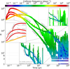 |
Fig. 4 Number N of moonlets as a function of time. The color is the frequency of collisions in collisions per day. It takes into account all moonlets. Simulations ran until t = 11 000 years. All simulations reach N < 10 but fragmentations can then temporarily grow N back to a few hundreds, as is seen by the spikes. Zoom-in of unclear parts of the figure are shown. |
3.4 Second stage of the formation: MMR
A well-known consequence of tides, important for our simulations, is the slow drift in semi-major axis that they provoke (Lainey et al. 2020). For an almost circular orbit, the semi-major axis increases (resp. decreases) when the mean motion is less (resp. more) than the sidereal rotation of Earth.
In the second stage of the formation, that starts a few years after the giant impact and lasts for thousands of years, the submoons that were formed during the first stage undergo tidal forces. Provided that their mean motion is less than the sidereal rotation of Earth, which is generally the case, they migrate away from Earth until they cross MMR or secular resonances. In the case of capture, these resonances lead either to the collisions of the submoons (e.g., Canup et al. 1999), and then to a completion of the formation of the Moon, or to the ejection of one or several of them from the system (capture by the solar system). It is also possible that resonance chains could be created, similar to Jupiter’s moons. Capture by a resonance are probably necessary to end up with a system that only contains one significant Moon. Indeed, unless two submoons have a close encounter early on, they end up on stable orbits and their mutual interactions average out without a MMR.
An example of two simulations that were affected by a MMR are “500b073S” and “500b075S”. In simulation “500b075S”, the two largest submoons entered the 2 : 1 MMR and the subsequent eccentricity increase allowed them to collide and complete the formation of the Moon. In simulation “500b073S” however, the two largest submoons entered the 5:1 MMR, leading to the ejection of one of them, preventing the growth of a full-size Moon.
Overall, when two submoons enter a MMR of the form p : q, the capture by the resonance is more likely to hinder the formation (by ejection) rather than to help it (by collision) when p/q is large. Indeed, in the p : q MMR, Kepler’s third law shows that the ratio between the semi-major axes is a2/a1 = (p/q)2/3. For the two submoons to collide and accrete, it is necessary that the apoapsis a1 (1 + e1) of the innermost gets beyond the periapsis a2 (1 - e2) of the outermost. When p/q is large, the semi-major axes are very different and it is unlikely that the submoons meet before one of them is ejected or disrupted by Earth’s tidal forces.
For example, in the 5 : 1 MMR, we have a2/a1 = 52/3 ≈ 2.924. Even if the capture in the 5 : 1 MMR leads to an eccentricity increase instead of an inclination increase, it is very unlikely that it would lead to the collision of the submoons. On one hand, if the eccentricity of the inner submoon increases significantly, then its periapsis goes below the Roche radius and it is disrupted by tidal forces. On the other hand, the eccentricity of the outer one would need to reach at least e2 = 0.658 for a close encounter to become possible. Even then, the close encounter can easily lead to the ejection of the already eccentric outer submoon by gravitational slingshot instead of a collision.
In Appendix B, we show an annex simulation, not in Table 1, where the capture in the 5 : 1 MMR led to the outer submoon leaving the equatorial plane. In this annex simulation, the two largest submoons ended up with a mutual inclination of ∼20°. This large mutual inclination, coupled with very different semimajor axes, made it very unlikely for the two submoons to collide before one of them is ejected from the system. Indeed, in this annex simulation, the outer one was ejected, preventing the formation of a full-size Moon and showing how MMR of the form p : q with a large value of p/q can hinder the formation of the Moon. In this appendix, we also study the 5 : 1 MMR from a more analytical point of view, and we refer the reader to Appendix B for a short overview of this MMR.
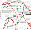 |
Fig. 5 Masses of the two most massive moonlets (black), of the inner fluid disk (red), and lost mass (green) as a function of time for all simulations. Some notable collisions (resp. escapes) are visible and can be related to Table 2 (resp. Fig. 1). |
4 Final state of our simulations
All four simulations mentioned in Table 1 led to the formation of at least a dwarf-size moon, and “500b075S” and “half-Earth” led to a fully grown moon. In these two simulations, the reason why a full-size moon was formed is different. In “half-Earth”, it is because there was only one major lunar seed initially (two are visible on Fig. 1 but one is quickly lost due to extreme orbital elements) on a close-in orbit. Therefore, all the material (coming from the inner fluid disk or from the N-body disk) accreted on that large seed and this simulation never featured two submoons of significant size. In “500b075S” however, a full-size moon was formed when the two largest submoons collided.
In Fig. 6, we plot the semi-major axis and mass of the largest submoon as a function of time. The collision that allowed a full-size moon to form in “500b075S” is visible, where a discontinuity in mass and semi-major axis is observed at time t ~ 500 years. In simulation “random”, although a collision between the largest submoon and a minor submoon occurred (visible at time t ~ 50 years), the second-largest submoon was lost around t ~ 580 years when it exited Earth’s Hill sphere. The associated loss of mass prevented a full-size moon to form.
In Sect. 3.4, we explained why MMR of the form p : q are more likely to hinder the formation of the Moon rather than to help it when p/q is large. This fact is visible in Fig. 7 where we plot the eccentricity of the largest submoon and the ratio between the mean motions of the two largest submoons as a function of time. On one hand, we can see that the collision that led to the formation of a full-size moon at time t ~ 500 years in simulation “500b075S” was due to the proximity to the low-order MMR 2:1. On the other hand, Fig. 7 shows that the formation of a full-size moon in simulation 500b073S was prevented by the high-order MMR 5 : 1.
In both Figs. 6 and 7, the capture of the dwarf moon of simulation “500b073S” by the evection resonance is visible. In Fig. 7, the capture is noticeable at time t ~ 2000 years when the eccentricity of the dwarf moon increased significantly until it reached 0.6 a thousand years later. In Fig. 6, the escape of the evection resonance is visible around t ~ 3000 years when the semi-major axis briefly decreased instead of increasing. This decrease in semi-major axis is because the eccentricity was high enough so that at periapsis, the instantaneous angular velocity of the dwarf moon exceeded the angular rotation of Earth and the dwarf moon was in front of the tidal bulge it raises on Earth. Since the dwarf moon was in front of its tidal bulge, it applied a positive torque on Earth’s rotation, and by conservation of the angular momentum, the dwarf moon semi-major axis decreased. When the dwarf moon was at apoapsis, the contrary happened, but then tides were very weak. Simulation “500b073S” is the only one with a capture by the evection resonance.
In Fig. 7, besides short-term variations due to close encounters, steady increases of the eccentricity are visible in all four simulations. These eccentricity increases are due to tidal forces. Indeed, when Ω/n > 18/11, where Ω is Earth’s sidereal rotation and n is the submoons’ mean motion, tides are responsible for an increase in eccentricity (e.g., Correia et al. 2012, Eq. (18)).
In Table 3, we present the state of the system at the end of each simulation (at time t = 11 000 years after the giant impact). The characteristics of the two submoons massive enough to be at hydrostatic equilibrium6 are presented in Table 4. Simulation “500b073S” features only one submoon at hydrostatic equilibrium and only that submoon is presented. The 12° inclination of the 0.069M☾ submoon of “half-Earth” is due to a capture into the 3:1 MMR with the 1.2M☾ Moon (teal color near the end of “half-Earth” in Fig. 7).
As expected, the mass of the proto-Earth increased slightly with respect to Table 1 due to material that fell onto it. Similarly, its length of day increased due to tides and the fact that almost all moonlets had periods larger than the length of day. For all simulations, the total mass in orbit around Earth decreased significantly between 40 hours after the giant impact (Mdisk in Table 1) and 11000 years after the giant impact (Mdisk in Table 3).
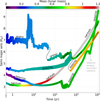 |
Fig. 6 Semi-major axis of the most massive submoon as a function of time for the simulations of Table 1. The color indicates the mass of the most massive submoon. |
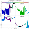 |
Fig. 7 Eccentricity of the most massive submoon as a function of time for the simulations of Table 1. The color shows the period ratio between the two most massive submoons. Notable MMR are indicated. Sudden color changes are ejections or collisions, whereas spikes correspond to close encounters. |
State of the system 11 000 years after the giant impact.
Two submoons at hydrostatic equilibrium.
5 Discussion
Because of the large mass loss throughout the evolution of the disk, we believe that the initial orbiting mass most likely to lead to a full-size Moon is ∼2M☾. However, SPH simulations of the canonical impact typically produce disks of mass ∼1.5M☾ or less, which is probably not enough. Simulation “500b075S” still led to an almost full-size moon, but we believe that it was not the most likely scenario7. With an orbiting mass of ∼1.5M☾ a few hours after the giant impact, a final moon of mass ∼0.65M☾, as is the case in simulation “500b073S”, is probably more likely. In simulation “500b075S”, the two most massive submoons were “lucky” enough to get captured in a low-order MMR (see Fig. 7). A statistical study of hundreds of simulations that combine SPH (for the first few hours after giant impact) and N -body (for the remaining thousands of years) would provide a more definite answer.
This contrasts with results of Canup et al. (1999) who found that when several submoons remain in the proto-lunar disk, they often merge via collision and an initial orbiting mass of ∼1.5 M☾ is enough to form a full-size Moon. However, in their work, submoons are captured in low-order MMR only (2:1, 3:2, or 3:1). As we showed in Sect. 3.4, captures in low-order MMR are less likely to lead to an ejection than captures in high-order MMR. Since MMR p : q is of order p - q in eccentricity, capture in high-order MMR require high eccentricity. As they use the results of Ida et al. (1997), who considered initially homogeneous and circular disks, it is possible that their submoons were formed less eccentric and therefore less prone to a capture into high-order MMR.
While more energetic, we do not find that the half-Earth model is, per se, more adapted to the formation of the Moon than the canonical model. However, we find that a giant impact yielding a disk mass larger than ∼2M☾ is the most adapted to the growth of a full-size Moon, because a lot of mass is lost through captures in high-order MMR and subsequent ejections, and ending up with a single object of mass ∼1 M☾ when the initial disk mass was less than 2M☾ is unlikely.
Since all canonical runs of Hull et al. (2024) generated disks of masses between 0.83 M☾ and 1.85 M☾ (see their Table 2), it is tempting to conclude that the canonical model is unadapted to the formation of a 1 M☾ Moon. However, it should be noted that in all of their runs, the impact velocity between the protoEarth and Theia is set exactly to the escape velocity of the pair. This velocity is only the lower bound of the actual velocity of the collision. Indeed, if υ∞ denotes the relative velocity between Theia and the proto-Earth before they enter each other’s Hill spheres, then the actual impact velocity is  . If the proto-Earth and Theia were on different orbits before the encounter, which was probably the case, then v∞ was a few km/s and the collision occurred with a velocity larger than vesc = 9.1 km/s chosen by Hull et al. (2024). Therefore, they are probably underestimating the amount of material put into Earth orbit8. As an example, if the proto-Earth was on a circular orbit with a = 1 AU and Theia on a slightly eccentric orbit with a = 1.25 AU and e = 0.2, then the encounter happened at Theia’s periapsis with v∞ = 2.85 km/s and the relative velocity at impact was 9.54 km/s, leading to an underestimation of the impact energy of ∼9%.
Previous N-body simulations of the Moon formation (e.g., Ida et al. 1997; Salmon & Canup 2012) suggest that in most cases, a single large Moon is formed within a few hundreds of years, and a second stage shaped by MMR is generally not needed. On the contrary, our work suggests that a second stage is often needed, because several significant submoons emerge from the first stage, one growing mainly with material from the inner fluid disk and another growing mainly from the N-body disk.
Unlike previous works, we find that the formation of the Moon is inefficient, in the sense that a large proportion of the proto-lunar disk’s mass is lost and not accreted onto the Moon. High-order MMR explain part of this inefficiency due to escapes of large submoons (discontinuities of the green curve in Fig. 5). The large number of moonlets featured in our simulations also favors the inefficiency, because small moonlets tend to acquire extreme orbital elements due to gravitational slingshot and are ejected more easily throughout the formation process. This is visible in Fig. 5 by the smooth increase of the green curve.
Overall, we still support the idea that the Moon likely formed from a disk subsequent to a giant impact involving the protoEarth. Despite not explaining the similar isotopic composition of Earth and the Moon, the canonical model remains the Ockham’s razor of the Moon’s presence around Earth. Furthermore, a canonical model with an impact velocity larger than 9.1 km/s, as aforementioned, would not only make the proto-lunar disk more massive, which favors a massive Moon, but would also mix better material from the upper layers of Earth with the disk, making the isotopic similarity between Earth and the Moon less problematic. Lastly, we will show in a coming paper that the Moon was probably not captured by the evection resonance. Since the canonical model forms the Earth-Moon system with the correct angular momentum, a capture by the evection resonance is not needed anymore to remove the excess, which is to be preferred.
6 Conclusion
In this work, we used the software NcorpiON to run N-body simulations of the formation of the Moon from a protolunar disk. The protolunar disk was subsequent to a giant impact between a Mars-sized Theia and the proto-Earth or between two half Earths, and our work was the first to consider initial conditions that are outputs of previous SPH simulations of the giant impact. We also considered randomly generated disks. In this paper, we presented in details four simulations, with very different outcomes.
Our model takes into account gravity between the moonlets, with Earth and with the Sun, the presence of an inner fluid disk below the Roche radius where tidal forces disrupt the moonlets, the equatorial bulge of Earth through the second zonal harmonic J2, and tides raised by the moonlets on Earth. In order to be able to consider disks with a large number N of moonlets, we computed the gravity between the moonlets using NcorpiON’s FalcON module that relies on fast multipole expansions. We chose FalcON parameters in such a way that 99% of moonlets had their acceleration computed with a relative error less than ∼0.04%. Secular resonances, such as the evection resonance, are taken into account in our work due to the Solar perturbations, and affect simulation “500b073S”. While the evection resonance is not investigated in this work, this is the purpose of a coming paper where we analyze the evection resonance with a novel analytical framework that we apply to the early Earth-Moon system.
More notably, our work on the Moon formation is the first to take into account fragmentations upon violent collisions between moonlets. NcorpiON and our simulations rely on the literature about crater scaling and ejecta models to develop a realistic model of fragmentation. Our simulations ran from a few hours after the giant impact up to 11 000 years, and featured 105 to 106 collisions in total. The catastrophicity of collisions in our simulations, defined in Sect. 3.2, spans over 15 orders of magnitude, from C ~ 10−10 (the colliding moonlets merge almost completely) up to C ~ 105 (the largest remnant has a mass ∼6 × 10⁻⁶ that of the total colliding mass).
Our simulations tend to suggest that the formation of the Moon likely happened in two distinct stages. The first stage started a few hours after the giant impact, when the protolunar disk had resolved into individual and probably liquid moon-lets. It lasted for a few years up to a few tens of years and was dominated by collisions (fragmentating or accreting) and gravitational scattering of moonlets. It was followed by a much longer second stage, that lasted 103 to 105 years, when several significant submoons, that formed during the first stage, migrated away from Earth due to tidal effects. This migration allowed them to encounter MMR, leading to collisions or ejections of submoons. At the end of the second stage, only one Moon remains and the inner fluid disk has been depleted.
In particular, we showed that during the second stage, highorder MMR are more likely to hinder the formation of the Moon by ejections, whereas low-order MMR are more likely to help it via collisions. The duration of the second stage is dependent on the submoons’ drift rate and thus on Earth’s tidal parameters after the impact, which are poorly known.
Several physical effects are not taken into account in our work, or lack realism. Gas drag, for instance, is disregarded as we assumed that all material in the disk is liquid. Considering drag should favor the fall of moonlets into the inner fluid disk and therefore contribute to make the innermost submoon bigger, at the detriment of farther submoons. Indeed, the innermost submoon mostly grows with material spawning from the inner fluid disk. We do not know how the overall formation of the Moon would be affected. As for our fragmentation model, it suffers from approximations and arbitrary decisions (Couturier et al. 2025, Sect. 5.3.) and should be refined to improve its degree of realism. Despite earlier works who showed that this effect is important (Meyer-Vernet & Sicardy 1987; Charnoz et al. 2011), gravitational interactions between the inner fluid disk and the moonlets, and subsequent torques, are also neglected in our work. A future attempt at a statistical study, as we roughly outline below, should consider taking into account this effect on top of fragmentations and a large number N of moonlets.
Finally, we showed the extreme chaoticity of the protolunar disk, with a Lyapunov timescale on the order of half an hour only. This justifies that regardless on our confidence on the initial conditions, a single simulation can only be interpreted as a possible scenario among others. Therefore, a solid future study of the formation of the Moon in the canonical model could be structured as follows:
Some ten SPH simulations of the impact between the proto-Earth and Theia with impact velocities in the range [9.1,10.4] km/s (0 ≤ v∞ ≤ 5 km/s) are run for ∼40 hours. Each SPH output is converted into an initial condition of N-body simulation (see Sect. 2.3), called parent initial condition;
From each parent initial condition, 100 children initial conditions are created by changing the speeds and positions of all moonlets by a tiny amount (Sect. 3.1).
Each child initial condition is simulated on NcorpiON for a few thousands years. Using FalcON with reasonable fragmentation thresholds (Sect. 2.4), each child simulation takes a few hours to a day on a single core;
With a ∼100 core cluster, each parent initial condition is therefore treated in a day and only ten days are needed to simulate all 1000 initial conditions.
From there, a statistical work can be carried out, revealing which parameters of the giant impact are more likely to form the Moon. Despite lacking a statistical study, our work suggests that an initial disk mass less than 2M☾ is unadapted to grow a full-size Moon. We favor the canonical model over others to explain the presence of the Moon.
Acknowledgements
J.C. carried out the numerical and analytical work, whereas A.Q. and M.N. provided ideas and insight. The authors declare that they do not have competing interests. J.C. thanks Scott D. Hull for providing output files of his SPH simulations. This work was partly supported by The National Aeronautics and Space Administration (NASA) grant numbers 80NSSC19K0514 and 80NSSC21K1184. M.N. thanks funding supports from the National Science Foundation (NSF) EAR-2237730 as well as the Center for Matter at Atomic Pressures (CMAP), an NSF Physics Frontier Center, under Award PHY-2020249. Any opinions, findings, conclusions or recommendations expressed in this material are those of the authors and do not necessarily reflect those of the National Science Foundation. M.N. acknowledges partial support by the Alfred P. Sloan Foundation under grant G202114194. J.C. acknowledges support of the Swiss National Science Foundation under grant number TMSGI2_211697.
References
- Barnes, J., & Hut, P. 1986, Nature, 324, 446 [NASA ADS] [CrossRef] [Google Scholar]
- Benz, W., & Asphaug, E. 1999, Icarus, 142, 5 [NASA ADS] [CrossRef] [Google Scholar]
- Boué, G., Correia, A. C. M., & Laskar, J. 2019, Astro Fluid 2016, 82, 91 [Google Scholar]
- Cameron, A. G. W., & Ward, W. R. 1976, LPSC, 7, 120 [Google Scholar]
- Canup, R. M. 2012, Science, 338, 1052 [NASA ADS] [CrossRef] [Google Scholar]
- Canup, R. M., & Asphaug, E. 2001, Nature, 412, 708 [Google Scholar]
- Canup, R. M., Levison, H. F., & Stewart, G. R. 1999, AJ, 117, 603 [Google Scholar]
- Canup, R. M., Righter, K., Dauphas, N., et al. 2023, Rev. Mineral. Geochem., 89, 53 [Google Scholar]
- Charnoz, S., Crida, A., Castillo-Rogez, J. C., et al. 2011, Icarus, 216, 535 [NASA ADS] [CrossRef] [Google Scholar]
- Correia, A. C. M., Boué, G., & Laskar, J. 2012, ApJ, 744, L23 [NASA ADS] [CrossRef] [Google Scholar]
- Couturier, J. 2022, PhD thesis, Observatoire de Paris, https://theses.hal.science/tel-04197740 [Google Scholar]
- Couturier, J., Quillen, A. C., & Nakajima, M. 2025, New Astron., 114, 102313 [Google Scholar]
- Cuk, M., & Stewart, S. T. 2012, Science, 338, 1047 [CrossRef] [Google Scholar]
- Dehnen, W. 2002, J. Computat. Phys., 179, 27 [CrossRef] [Google Scholar]
- Dehnen, W. 2014, Comput. Astrophys. Cosmol., 1, 1 [NASA ADS] [CrossRef] [Google Scholar]
- Gastineau, M., & Laskar, J. 2011, ACM Commun. Comput. Algebra, 44, 194 [Google Scholar]
- Goldreich, P., & Ward, W. R. 1973, ApJ, 183, 1051 [Google Scholar]
- Hartmann, W. K., & Davis, D. R. 1975, Icarus, 24, 504 [NASA ADS] [CrossRef] [Google Scholar]
- Housen, K. R., & Holsapple, K. A. 2011, Icarus, 211, 856 [NASA ADS] [CrossRef] [Google Scholar]
- Hull, S. D., Nakajima, M., Hosono, N., Canup, R. M., & Gassmöller, R. 2024, Planet. Sci. J., 5, 9 [Google Scholar]
- Hull, S. D., Nakajima, M., Canup, R. M., Visscher, C., & Sossi, P. A. 2026, Icarus, 450, 116940 [Google Scholar]
- Ida, S., Canup, R. M., & Stewart, G. R. 1997, Nature, 389, 353 [NASA ADS] [CrossRef] [Google Scholar]
- Jutzi, M., Michel, P., Benz, W., & Richardson, D. C. 2009, Icarus, 41, 50.06 [Google Scholar]
- Kokubo, E., & Ida, S. 2000, Icarus, 143, 15 [Google Scholar]
- Kokubo, E., Ida, S., & Makino, J. 2000, Icarus, 148, 419 [NASA ADS] [CrossRef] [Google Scholar]
- Lainey, V., Casajus, L. G., Fuller, J., et al. 2020, Nat. Astron., 4, 1053 [Google Scholar]
- Laskar, J., & Gastineau, M. 2009, Nature, 459, 817 [NASA ADS] [CrossRef] [Google Scholar]
- Laskar, J., & Robutel, P. 1995, Celest. Mech. Dyn. Astron., 62, 193 [Google Scholar]
- Leinhardt, Z. M., & Stewart, S. T. 2012, ApJ, 745, 79 [NASA ADS] [CrossRef] [Google Scholar]
- Lock, S. J., Stewart, S. T., Petaev, M. I., et al. 2018, J. Geophys. Res.: Planets, 123, 910 [Google Scholar]
- Meyer-Vernet, N., & Sicardy, B. 1987, Icarus, 69, 157 [Google Scholar]
- Mignard, F. 1979, Moon Planets, 20, 301 [Google Scholar]
- Nakajima, M., Genda, H., Asphaug, E., & Ida, S. 2022, Nat. Commun., 13, 568 [Google Scholar]
- Nakajima, M., Atkins, J., Simon, J. B., & Quillen, A. C. 2024, Planet. Sci. J., 5, 145 [Google Scholar]
- Nduka, A. 1971, ApJ, 170, 131 [Google Scholar]
- Rein, H., & Liu, S.-F. 2012, A&A, 537, A128 [NASA ADS] [CrossRef] [EDP Sciences] [Google Scholar]
- Roberts, J. H., & Nimmo, F. 2008, Icarus, 194, 675 [Google Scholar]
- Rufu, R., & Canup, R. M. 2020, J. Geophys. Res.: Planets, 125, e2019JE006312 [Google Scholar]
- Rufu, R., Aharonson, O., & Perets, H. B. 2017, Nat. Geosci., 10, 89 [NASA ADS] [CrossRef] [Google Scholar]
- Saillenfest, M., Rogoszinski, Z., Lari, G., et al. 2022, A&A, 668, A108 [NASA ADS] [CrossRef] [EDP Sciences] [Google Scholar]
- Salmon, J., & Canup, R. M. 2012, ApJ, 760, 83 [Google Scholar]
- Singer, S. F. 1968, Geophys. J. Roy. Astron. Soc., 15, 205 [Google Scholar]
- Sossi, P. A., Nakajima, M., & Khan, A. 2024, Composition, Structure and Origin of the Moon [Google Scholar]
- Stewart, S. T., & Leinhardt, Z. M. 2009, ApJ, 691, L133 [NASA ADS] [CrossRef] [Google Scholar]
- Suetsugu, R., Tanaka, H., Kobayashi, H., & Genda, H. 2018, Icarus, 314, 121 [NASA ADS] [CrossRef] [Google Scholar]
- Touma, J., & Wisdom, J. 1998, AJ, 115, 1653 [NASA ADS] [CrossRef] [Google Scholar]
- Wahr, J. 1996, Geodesy and Gravity (Samizdat Press) [Google Scholar]
- Ward, W. R., Canup, R. M., & Rufu, R. 2020, J. Geophys. Res.: Planets, 125, e2019JE006266 [Google Scholar]
- Zahnle, K. J., Lupu, R., Dobrovolskis, A., & Sleep, N. H. 2015, Earth Planet. Sci. Lett., 427, 74 [CrossRef] [Google Scholar]
- Zhang, J., Dauphas, N., Davis, A. M., Leya, I., & Fedkin, A. 2012, Nat. Geosci., 5, 251 [NASA ADS] [CrossRef] [Google Scholar]
The equatorial bulge invalidates this hypothesis.
This quantity determines how far apart cells must be for their mutual gravity to be treated via a multipole expansion.
Semi-major axis, eccentricity, inclination; true anomaly, argument of the periapsis, longitude of the ascending node.
NcorpiON uses REBOUND's 3D viewer (Rein & Liu 2012).
We considered Mimas’ mass as a threshold.
To be proven by a statistical study in a future work.
Although the additional material is not necessarily bounded to Earth.
Appendix A Notations
We gather for convenience all the notations used throughout this work in Table A.1.
Appendix B The 5 : 1 MMR
The 5 : 1 MMR is a high-order MMR that could have played a role during the second stage of the Moon formation (see Sect. 3.4). We elaborate here the framework of a Hamiltonian description of this resonance.
We consider two submoons of mass m1 (inner) and m2 (outer) orbiting Earth. The Hamiltonian is H = HK + HP, where the perturbative part HP is due to gravitational interactions between the submoons, and the Keplerian part, due to submoon-Earth interactions, reads
 (B.1)
(B.1)
with μj = G(M⊕ + mj and βj = M⊕mj/(M⊕ + mj). We define λj the mean longitude of submoon j, ϖj the longitude of its periapsis, and Ωj the longitude of its ascending node. We work with Poincaré’s canonical variables (Λj, Dj, Zj; λj, -ϖj, -Ωj), where λj is conjugated to the circular angular momentum  is conjugated to the angular momentum deficit (AMD)
  and -Ωj is conjugated to the third component of the angular momentum
  .
.
Considering that the system is close to the 5 : 1 MMR, we only retain terms in the Fourier decomposition of the Hamiltonian that depend on a multiple of the slow angle λ1 - 5λ2. Using Laskar & Robutel (1995) and truncating to fourth order in eccentricity and inclination, d’Alembert rule shows that HP can be written
 (B.2)
(B.2)
where  and
and  . The coefficients Cl(α) depend on the Laplace coefficients. In Table B.1, we give for reference the 19 coefficients appearing in Eq. (B.2). We obtained their expression as a function of the Laplace coefficients using the algebraic manipulator TRIP (Gastineau & Laskar 2011). Since the system is in the 5:1 MMR, a good approximation is to evaluate them at α = (1/5)2/3 and to consider them constant.
The system currently has 6 degrees of freedom, which are (Λj, Dj, Zj; λj, -ϖj, -Ωj) for 1 ≤ j ≤ 2. Since the system stays close to the resonance 1 : 5, a suitable change of variable is
 (B.3)
(B.3)
This transformation is canonical with the new actions Φ1 = (5Λ1 + Λ2)/4 conjugated to φ1 and Φ2 = Σj(Λj - Dj - Zj) conjugated to ϕ2. The actions Dj and Zj are unchanged, and Dj (resp. Zj) is conjugated to σj (resp. ςj). Since the Hamiltonian has been averaged over the fast angle φ1 (by only keeping contributions depending on λ1 - 5λ2 in the perturbation), the action Φ1 is a first integral of the averaged problem. Furthermore, since Φ2 is the third component of the total angular momentum and is also a first integral, its conjugated angle φ2 does not appear in the Hamiltonian. The problem is reduced to the four degrees of freedom (Dj, Zj; σj, ςj). This change of variable is easily applied to the Hamiltonian, since a generic cosine term now reads
 (B.4)
(B.4)
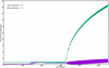 |
Fig. B.1 Inclination of the two largest moonlets of an annex simulation. The capture into the 1 : 5 MMR leads to a large increase of the mutual inclination. |
In Fig. (B.1), we show the mutual inclination between the two largest submoons of an annex simulation similar to "500b073S". This simulation is not part of Table 1 but it shows how a highorder MMR can hinder the formation of the Moon. In Fig. (B.1), the submoons enter the 5 : 1 MMR, leading to a significant increase in the inclination of the outermost submoon, while the innermost submoon is locked to the equatorial plane due to the J2 (Saillenfest et al. 2022, Eq. (2)) and only experiences a moderate inclination increase. In this annex simulation, as in simulation "500b073S", the outer submoon was eventually ejected. In Fig. B.2, we show the time evolution of the four angles (σ1, σ2, ς1,ς2).
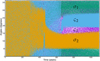 |
Fig. B.2 Four angles (σ1,σ2,ς1,ς2) of the 5:1 MMR for the annex simulation presented in Fig. B.1. At time t = 650 years, the significant increase in the inclination of the outer submoon corresponds to the moment when the angle ς2, conjugated to the inclination of the outer submoon, starts to librate. |
Notations used in this paper
We know that the inclination increase is due to a capture by the 5 : 1 MMR because at time t = 650 years, right when the outermost submoon’s inclination started to increase, the angle ς2 = −λ1/4 + 5λ2/4 − Ω2, conjugated to the inclination of the outermost submoon, started to librate (light blue in Fig. B.2).
All Tables
All Figures
|
Fig. 1 3D visualization of the initial conditions. Moonlets are displayed six times bigger than they actually are, whereas Earth is displayed with its true radius and indicates the scale. The red cross is the center of mass of the system and is inside Earth. The masses and orbital elements of notable moonlets are indicated. Some have highly eccentric orbits and are quickly lost. |
| In the text | |
|
Fig. 2 Distance between the two farthest simulations in the phase space and in the position space and best exponential fit. The discontinuities in the black curve come from elastic collisions. The exponential fits the green curve. |
| In the text | |
|
Fig. 3 Distribution of the catastrophicities of all collisions that occurred in our four runs. Run “500b073S”, “500b075S”, “half-Earth” and “random” had 163 202, 283 957, 539 143 and 1 000 405 collisions, respectively. Links to logs of all collisions for the four simulations are given in Table 4. |
| In the text | |
|
Fig. 4 Number N of moonlets as a function of time. The color is the frequency of collisions in collisions per day. It takes into account all moonlets. Simulations ran until t = 11 000 years. All simulations reach N < 10 but fragmentations can then temporarily grow N back to a few hundreds, as is seen by the spikes. Zoom-in of unclear parts of the figure are shown. |
| In the text | |
|
Fig. 5 Masses of the two most massive moonlets (black), of the inner fluid disk (red), and lost mass (green) as a function of time for all simulations. Some notable collisions (resp. escapes) are visible and can be related to Table 2 (resp. Fig. 1). |
| In the text | |
|
Fig. 6 Semi-major axis of the most massive submoon as a function of time for the simulations of Table 1. The color indicates the mass of the most massive submoon. |
| In the text | |
|
Fig. 7 Eccentricity of the most massive submoon as a function of time for the simulations of Table 1. The color shows the period ratio between the two most massive submoons. Notable MMR are indicated. Sudden color changes are ejections or collisions, whereas spikes correspond to close encounters. |
| In the text | |
|
Fig. B.1 Inclination of the two largest moonlets of an annex simulation. The capture into the 1 : 5 MMR leads to a large increase of the mutual inclination. |
| In the text | |
|
Fig. B.2 Four angles (σ1,σ2,ς1,ς2) of the 5:1 MMR for the annex simulation presented in Fig. B.1. At time t = 650 years, the significant increase in the inclination of the outer submoon corresponds to the moment when the angle ς2, conjugated to the inclination of the outer submoon, starts to librate. |
| In the text | |
Current usage metrics show cumulative count of Article Views (full-text article views including HTML views, PDF and ePub downloads, according to the available data) and Abstracts Views on Vision4Press platform.
Data correspond to usage on the plateform after 2015. The current usage metrics is available 48-96 hours after online publication and is updated daily on week days.
Initial download of the metrics may take a while.