| Issue |
A&A
Volume 708, April 2026
|
|
|---|---|---|
| Article Number | A309 | |
| Number of page(s) | 10 | |
| Section | Planets, planetary systems, and small bodies | |
| DOI | https://doi.org/10.1051/0004-6361/202558649 | |
| Published online | 21 April 2026 | |
Solar System material reaching neighboring star systems
1
Astronomical Institute, Slovak Academy of Sciences,
05960
Tatranská Lomnica,
Slovakia
2
Faculty of Mathematics, Physics, and Informatics, Commenius University,
Bratislava,
Slovakia
3
Astronomical Institute, Slovak Academy of Sciences,
Bratislava,
Slovakia
★ Corresponding author: This email address is being protected from spambots. You need JavaScript enabled to view it.
Received:
18
December
2025
Accepted:
10
March
2026
Abstract
Context. In our Solar System, few macroscopic objects have been observed to be moving in hyperbolic orbits and, thus, they must have originated from interstellar space. Some meteoroids are also suspected to have an interstellar origin. Analogously, some cometary nuclei have left the Solar System and a similar behavior can be expected for a number of meteoroids.
Aims. We investigate whether meteoroids ejected from the Solar System have the capacity to reach neighboring stars in the future. We also study the minimum distances between these stars and real comets that have managed to escape the Sun’s potential.
Methods. The trajectories of hypothetical meteoroid particles and real cometary nuclei were integrated numerically. To estimate the precision of the integration, we simultaneously used two integration algorithms: the Runge-Kutta method and the symplectic integrator known as Leapfrog. We employed the CNS5 catalog of neighboring stars and the CODE catalog of future orbits of comets.
Results. Since the heliocentric speeds of the meteoroids leaving the Solar System are relatively low, only 5 of the 3893 considered stars can be approached by these meteoroids within 10 au. The other stars are too fast and end up escaping from the vicinity of the system before any particle approaches their innermost region. Of the 123 considered comets, 14 are predicted to approach a star within 50 000 au during the next 5 Myr, but none of them will end up closer than 4633 au. Because of the relatively large uncertainty of the determination of input parameters of considered stars, our result unfortunately suffers from a large uncertainty.
Conclusions. Our results indicate that only a very small amount of material from the Solar System can be delivered to the systems of neighboring stars.
Key words: comets: general / meteorites, meteors, meteoroids / stars: general / ISM: kinematics and dynamics
© The Authors 2026
 Open Access article, published by EDP Sciences, under the terms of the Creative Commons Attribution License (https://creativecommons.org/licenses/by/4.0), which permits unrestricted use, distribution, and reproduction in any medium, provided the original work is properly cited.
This article is published in open access under the Subscribe to Open model. This email address is being protected from spambots. You need JavaScript enabled to view it. to support open access publication.
1 Introduction
The motion of the Sun through the galactic environment inevitably results in the presence of interstellar material in the Solar System. The presence of interstellar dust from the Local Interstellar Cloud (LIC) has been confirmed by detections made with dust instruments on board spacecrafts (from several NASA and ESA missions) at distances of only a few astronomical units (au) from the Sun (Grün et al. 1993; Krüger et al. 2007). The dust may even be present around Earth’s orbit (Altobelli et al. 2003; Strub et al. 2019). Interstellar dust has been measured both at high ecliptic latitudes (e.g., Gruen et al. 1994; Sterken et al. 2015) and in the ecliptic plane (Baguhl et al. 1995; Colwell et al. 1998).
Larger interstellar particles, not coupled to the LIC, but originating from other stellar systems, have also been reported to enter the Earth’s atmosphere as meteoroids (e.g., Baggaley et al. 1993; Hawkes & Woodworth 1997; Meisel et al. 2002; Peña-Asensio et al. 2022). However, none of these cases can be regarded as unambiguously confirmed due to the limited accuracy of meteor observations (Musci et al. 2012; Hajduková et al. 2020; Barghini et al. 2025). Therefore, the proportion of interstellar particles relative to the local population remains unknown (Hajduková et al. 2019; Wiegert et al. 2025), with their flux estimated to be very low (e.g., Landgraf et al. 2000; Weryk & Brown 2004; Hajduková & Hajduk 2006; Froncisz et al. 2020; Wiegert et al. 2025). This makes it unclear whether their absence reflects the properties of the interstellar environment, results from size-dependent limited lifetimes, or is merely a consequence of measurement constraints.
The presence of free-floating bodies in the interstellar space is, however, a natural byproduct of planetary system formation. Likely forming denser streams (Portegies Zwart 2021), they orbit within the Galaxy and may encounter neighboring stars. Such moving groups, however, represent a transient location in velocity space rather than the origin of the objects (Hopkins et al. 2025a). Thus, due to radial migration, interstellar objects observed in the Solar System are expected to originate from stars of all ages, reflecting their formation throughout the Galactic disk (Hopkins et al. 2025a). Three such objects ejected from distant stellar systems were distinctly identified as they passed through our Solar System (Meech et al. 2017; Guzik et al. 2020; Seligman et al. 2025). Their dynamical paths back to their original stellar systems are, however, unknown because of limitations in current observational data and in numerical integration methods, which lead to large uncertainties (Zhang 2018; Bailer-Jones et al. 2018; Hallatt & Wiegert 2020). Nevertheless, there are dynamical studies that have proposed plausible candidate source systems for them (e.g., Gaidos et al. 2017; Dybczyński & Królikowska 2018).
Given the uncertainty in the data, only a few attempts have been made to characterize possible meteoroid streams arriving from specific interstellar directions (Baggaley & Neslušan 2002). The existence of an interstellar stream from Beta Pictoris was suggested by Baggaley (2000), but the reported parameters were later shown to be incorrect (Murray et al. 2004). More recently, Gregg & Wiegert (2025a) studied several known nearby debris-disk stars, including Beta Pictoris, and concluded that material from these systems can reach the Solar System. Their models have provided the characteristics of the resulting interstellar streams, which could aid in identifying interstellar meteors. The authors also reported a possible influx of meteoroids from the Alpha Centauri system (Gregg & Wiegert 2025b).
In this work, we address the opposite scenario. Our aim is to determine whether material ejected from the Solar System can reach other stellar systems in the Sun’s vicinity. We consider (1) a hypothetical sample of meteoroids and (2) a sample of known hyperbolic comets whose orbits have been determined with a higher level of accuracy. Here, we model their ejections from the Solar System at present and track their dynamical evolution to reveal their eventual close approaches to nearby stars.
The paper is organized as follows. In Sect. 2 we discuss dynamical properties of stars used in our analysis, introducing the sample of nearby stars (Sect. 2.1), the Galactic potential (Sect. 2.2), and the numerical integration of stellar orbits (Sect. 2.3). In Sect. 3, we present the sample of hyperbolic comets (Sect. 3.1) and the straight-line approximation of trajectories of small bodies escaping the Solar System (Sect. 3.2). In Sect. 4, we analyze future close approaches between small bodies leaving the Solar System and nearby stars, focusing on theoretical meteoroids (Sect. 4.1) and real hyperbolic comets (Sect. 4.2). We discuss the impact of measurement uncertainties on our work in Sect. 5 and summarize the obtained results in Sect. 6.
2 Dynamical properties of nearby stars
2.1 Adopted database of stars
To investigate the approach of a particle to a neighboring star, we need to know the dynamical characteristics of the star. These characteristics include the heliocentric radius and velocity vectors. In some cases, the focusing effect of the stellar gravity may be important and, therefore, we also need to know the mass of the star.
To obtain the complete set of the dynamical characteristics, we used the updated CNS5 catalog1 (Golovin et al. 2023), which provides the most complete sample of all known stars and brown dwarfs within 25 parsecs of the Sun (5 931 objects). From this sample, we selected only stars with the complete dynamical characteristics (i.e., position on the sky, stellar parallax, proper motion in right ascension, proper motion in declination, and radial velocity), leaving us with a final sample of 3 893 objects. The determination errors of parallaxes, proper motions and radial velocities are also given.
The inputs into the integration are the rectangular Galactocentric position and velocity vectors. To calculate these vectors for the stars, we firstly transformed the parameters to the rectangular heliocentric vectors. Since the directional parameters in the catalog are given in equatorial coordinate frame, the rectangular components x*o, y*o, and z*o of the radius-vector of star will also be given, in the first step, in this frame.
In the catalog, the parameters characterizing the stars are referred to four various epochs: 1991.25 (2 stars), 2000.0 (5 stars), 2015.5 (5 stars), and 2016.0 (the remaining 3881 stars). The epoch is related to the time for which the observational characteristics were determined. A given star, however, would have possessed these characteristics in time to = r*/c before the epoch (r* is the distance of the star and c is the speed of light). Given this circumstance, we unified the stellar data calculating the heliocentric radius and velocity vectors characterizing a given star in common time, whereby we chose the time on January 1.0, 2000 (JD=2451544.5). In particular, we performed the numerical integration for the time equal to JD2451544.5 − JD(epoch) + r*/c. The final radius and velocity vectors were regarded as the true vectors in the common nominal epoch of JD2451544.5. We note that when referring to the particular star throughout this paper, we quote the CNS5 designation (cns5_id) throughout.
To assign stellar masses for those objects, we cross-matched this sample with the TESS input catalog (Stassun et al. 2018) version 8.2 (Paegert et al. 2021), obtaining masses for 3517 objects. The Gaia FLAME masses (Creevey et al. 2023) were available only for 565 objects. In total, this left us with 3 545 objects with both full dynamical characteristics and mass estimates. We followed the motion of stars and Sun in the Galaxy via a numerical integration of their trajectories (see Sect. 2.3).
2.2 Gravitational potential of the Galaxy in solar neighborhood
It is widely known that all nearby stars currently pass the Solar System in straight-line (or nearly straight-line) trajectories. This condition was used in a calculation of the stellar perturbations on the cometary nuclei in the Oort Cloud (Rickman 1976; Dybczynski 1994). However, a stellar trajectory can be well approximated by a straight line only in close vicinity to the Sun, on a scale comparable with the diameter of the Oort Cloud (about a half a parsec). The length of the trajectory when its bending due to the gravity of the Milky Way becomes significant is not known; however, we do know that it is not unique, as it depends on the speed of given star. Since our aim is to study a motion of material also beyond the region of the Sun’s domination, we need to know the stellar trajectory better than approximated by a straight line. This knowledge can be gained only by a following of the stellar motion in the Galaxy.
In this work, we employ the description of the Milky Way large-scale gravitational potential first described by García-Sánchez et al. (2001). It comprises three components of net gravity: the Galactic bulge, halo, and disk. We do not include the gravity from the spiral arms in our integration, as it spans a relatively short time and, thus, it is not required. We assume that the differential action on a star and Sun from the neighboring arm is negligible. An uncertainty of knowledge of gravitationally effective distance from the arm would probably be larger than the effect of the differential action.
To describe a motion of star as well as the Sun in the Galaxy, we can consider the modified rectangular Galactocentric coordinate frame (see Fig. 1), with its x-axis oriented away from the Galactic center and passing through the projection point of the Sun on the Galactic mid-plane at the start of a time period (t = 0). The y-axis is oriented in the sense of Galactic rotation and z-axis oriented toward the South Galactic Pole to retain the right-handed system. We denote the distance of the projection point of the Sun to the Galactic mid-plane from the center of the Galaxy in t = 0 as R⊙ and the Sun’s distance from the mid-plane of the Galactic disk as z⊙. Since the Sun is currently situated above the plane and the positive orientation of the coordinate z-axis is directed toward the South Pole, the value of z⊙ is negative.
Based on the characteristics of stars in the catalog, we know the heliocentric common-galactic coordinates of stellar radius-vector, x*o, y*o, z*o, and velocity-vector, v*x, v*y, and v*z. We transformed these vectors to the used modified Galactocentric coordinates and velocities. The test particles representing the hypothetical meteoroids or cometary nuclei are also characterized in this coordinate frame. In this section, we employ a general denotation of the radius vector as r = (x, y, z) and velocity vector as v = (vx, vy, vz) in this frame. The components of the velocity-vector of the Sun in the Local Standard of Rest are denoted as v⊙x, v⊙y, and v⊙z. The angular speed of the Galaxy rotation in the region of the current Sun’s position is denoted by Ω⊙. The numerical values characterizing the position and velocity of the Sun, taken from (García-Sánchez et al. 2001), are given in Table 1.
The components of the Milky Way’s gravitational potential were given in the cylindrical coordinate frame with the radial component, ![Mathematical equation: $\[R~\left(R=\sqrt{x^{2}+y^{2}}\right)\]$](/articles/aa/full_html/2026/04/aa58649-25/aa58649-25-eq4.png) , and component, z, being perpendicular to the Galactic mid-plane and oriented toward the Galactic South Pole.
, and component, z, being perpendicular to the Galactic mid-plane and oriented toward the Galactic South Pole.
For the spherically symmetric halo and bulge components, we adopted Plummer’s model (Plummer 1911). For the halo, the potential is given as
![Mathematical equation: $\[\Phi_h=\frac{G M_h}{\sqrt{R^2+z^2+b_h^2}},\]$](/articles/aa/full_html/2026/04/aa58649-25/aa58649-25-eq5.png) (1)
(1)
where G is the gravitational constant, Mh is the mass of halo within the radius, R, and bh is a constant. The same formula is valid for the potential of bulge when the subscript h in the denotation of mass and constant parameter is replaced with the subscript b; then, Mb is the mass of the bulge and bb is a constant related to this entity. The numerical values of the masses and constant parameters, again taken from (García-Sánchez et al. 2001), are given in Table 1.
For the axisymmetric Galactic disk, the Miyamoto & Nagai (1975) form of the Kuzmin model (Kuzmin 1956) was adopted in accordance with the García-Sánchez et al. considerations. In this model, the gravitational potential of the disk is given as
![Mathematical equation: $\[\Phi_d=\frac{G M_d}{\sqrt{R^2+\left(a_d+\sqrt{z^2+b_d^2}\right)^2}}.\]$](/articles/aa/full_html/2026/04/aa58649-25/aa58649-25-eq6.png) (2)
(2)
In this relation, Md is the mass of the disk, while ad and bd are constant parameters characterizing the disk. We recall that the numerical values of all these constants, presented by García-Sánchez et al. (2001), can be found in Table 1.
 |
Fig. 1 Position of a star characterized in the heliocentric (x*, y*, z*) and modified-galactic (x, y, z) coordinate frames. Abbreviation GC denotes the Galactic center. |
Parameters of the used model of Galactic gravitational potential.
2.3 Numerical integration of stellar orbits
We used a relatively fast, symplectic, integration algorithm known as Leapfrog (Duncan et al. 1998). Since we had no information about the reliability of this integration in an application similar to ours, we checked the result by an independent integration method. Specifically, we also used, in some demonstrative cases, the Runge-Kutta integration algorithm. It is highly improbable that two independent methods would result in the same erroneous values. Therefore, if the results of both methods are the same, we can regard them as reliable.
At the beginning of Sect. 2.2, we stated that the stellar trajectories can be well approximated by a straight line, when the perturbations of the passing stars on the cometary nuclei in the Oort Cloud are investigated. To find when the difference between a position of a star in the straight-line trajectory and along its actual trajectory influenced by Galactic gravity becomes significant, we compared the positions of all stars in our sample as calculated (i) considering the uniform, straight-line motion and (ii) trajectories influenced by the Galaxy.
The largest difference in the position as well as in the velocity occurred for star No. 1475. The increase in the differences over 1 Myr is shown in Figs. 2a, b. As expected, the difference mostly increased in the x-component that was initially oriented outward from the Galactic center (i.e., in the radial direction in respect to the Galaxy).
In the context of our investigation, we are interested in the heliocentric distances and velocities of the stars. Since the Galactic gravity also influences the motion of the Sun, the differences in the heliocentric position and heliocentric velocity are not the same as those related to the absolute galactic coordinate frame. The differences relative to the Sun are much smaller, as documented in plots c and d of Fig. 2. However, the maximum heliocentric differences were not those reported for star No. 1475; rather, the maximum heliocentric distance was found for star No. 2857 (Fig. 2e) and the maximum heliocentric velocity was found for star No. 5497 (Fig. 2f).
In any case, the differences in the maximum heliocentric distance, as well as the maximum heliocentric speed seem to be significant already on a time scale of several hundred millennia, which is the subject of our investigation. Hence, we are forced to follow the motion of the stars and Sun as influenced by the gravity of the Milky Way; in particular, the straight-line trajectories are not a sufficient approximation, although the straight-line approximation can still be useful in providing us with the initial velocity vector in an iteration (see Sect. 4).
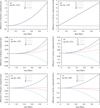 |
Fig. 2 Difference in the position (panels a, c, and e) and velocity (b, d, and f) when the stellar trajectory is calculated as (i) a trajectory of uniformly moving object along a straight line and (ii) a trajectory of the object gravitationally perturbed by the Milky Way. Panels a and b: Maximum detected differences in the galactic coordinate frame. The maximum occurred as for the distance as velocity in the case of star No. 1475. Panels c and d: Differences in the heliocentric coordinate frame of this star. In this frame, the maximum was not detected for this star and, instead, the heliocentric distance maximum for star No. 2857 (e) and the heliocentric velocity maximum for star No. 5497 (f) were detected. The modified galactic coordinate system, with the x-axis oriented outward from the Galactic center, is adopted. |
3 Dynamical properties of small bodies escaping the Solar System
3.1 Sample of hyperbolic comets
In meteor databases, many particles appear to move on hyperbolic orbits. However, a prevailing majority of these particles (and possibly all of them) are considered to be in hyperbolic orbits due to a poor accuracy of the determination of their heliocentric orbits (Hajduková et al. 2019). These hyperbolic orbits do not provide any relevant information about interstellar material or about material that actually ends up escaping the Solar System. In fact, it is only a negligible fraction of meteoroids locally accelerated to hyperbolic orbits that end up approaching the Earth’s orbit and that might, thus, be observed as meteors (Wiegert 2014).
The orbits of comets are determined with a much better precision. Królikowska & Dybczyński (2023) published the catalog named CODE, containing the future orbits of 123 hyperbolic comets. The future orbits in this catalog are osculating orbits of the objects in the heliocentric distance of 250 au, when they leave the Solar System. Those authors determined some orbits under various assumptions. Hence, there are two or more orbits for some comets. The solutions are labeled as: pa, pc, pd, bt, ra, and so we refer to their paper for more details. The resulting orbits were not, however, significantly different and the authors did not discriminate between the quality of these solutions. Therefore, we simply considered the first hyperbolic solution for given comet in their table when constructing the directional distribution of outbound asymptotes and distribution of heliocentric speed in a large heliocentric distance (Figs. 3 and 4).
This catalog can be used to map a directional distribution of the escaping comets and the hyperbolic excess of their velocity (i.e., the heliocentric speed they had at an infinite heliocentric distance when travelling on the current hyperbolic orbit). In Fig. 3, we can see that the comets leave the Solar System randomly in all directions. The velocity excess is typically small, lower than ~1.6 km s−1, but mostly (in 90%) lower than 0.9 km s−1 (Fig. 4). The extraordinarily fast comet, C/1980 E1, having a velocity excess of 3.8 km s−1 is not shown in Fig. 4. There are several peaks in the speed distribution. These could occur due to a statistical fluctuation or perhaps due to the effects of some action exerted by a giant planet (or several giant planets).
There is no reason to assume a different directional or speed distribution of meteoroids in comparison with those of the cometary nuclei, since we can expect that the meteoroids that are able to leave the Solar System end up gaining their hyperbolic velocity due to the same mechanism (i.e., gravitational perturbations by the giant planets) as the hyperbolic comets. A significant part of them is obviously released just from the hyperbolic comets during their passage through the inner region of our planetary system. In our modeling, we thus considered a random distribution of the direction of modeled test particles and set of discrete, equidistant values of escaping speeds: vi = 0.25, 0.50, 0.75, 1.00, 1.25, and 1.50 km s−1 for i = 1, 2, 3, 4, 5, and 6.
Some microscopic meteoroids are likely to move faster due to non-gravitational acceleration. However, they must be affected by the non-gravitational forces also in interstellar space. Since, these forces are practically impossible to predict, we did not consider any of the unknown dynamics of such small particles. In any case, their contribution to the total delivered material to an alien stellar system can be expected negligible.
 |
Fig. 3 Directions of the outbound asymptotes of the hyperbolic orbits of 123 comets leaving the Solar System in the Hammer projection of celestial sphere. The ecliptic coordinate frame is used. |
 |
Fig. 4 Distribution of the speed in an infinite heliocentric distance of the hyperbolic orbits of 122 comets leaving the Solar System. The speed of comet C/1980 E1 was 3.8 km s−1 and exceeds the shown interval. |
3.2 Straight-line approximation
The trajectory of a star or test particle in the galactic coordinate frame can be roughly approximated by a straight line during the predicted time of encounter, which was found to be lower than ~4 Myr (and predominantly lower than ~1.4 Myr). Hence, the velocity vector of a meteoroid, that is expected to approach a given star in a near future, can be roughly estimated (in an analytical way) when we consider the motion of the meteoroid and star along the straight-line trajectories with a constant velocity. In the following, we describe the calculation of the appropriate velocity vector of the meteor.
We can consider a star in the position characterized at the time, t = 0, with the heliocentric radius-vector of r*o = (x*o, y*o, z*o). The star moves with the constant velocity, which is characterized with v*o = (v*ox, v*oy, v*oz) in the considered heliocentric galactic coordinate frame. Since we are using the modified galactic coordinates in the calculation of the perturbed motion, the stellar radius and velocity vectors in the latter coordinate system would then be r* = (x*, y*, z*) = (−x*o, y*o, z*o) and v* = (v*x, v*y, v*z) = (−v*ox, v*oy, −v*oz). The position of the star at the time, t, will obviously be
![Mathematical equation: $\[\boldsymbol{r}_*=\boldsymbol{r}_{* O}+\boldsymbol{v}_* t.\]$](/articles/aa/full_html/2026/04/aa58649-25/aa58649-25-eq7.png) (3)
(3)
The test particle, representing the meteoroid that will approach the star, is initially located in the center of the considered heliocentric coordinate frame: ro = (xo, yo, zo) = (0, 0, 0). The particle will approach the star when its velocity will be characterized with the appropriate velocity vector v = (vx, vy, vz) in the heliocentric modified galactic coordinate system. Moving with the velocity characterized by this vector, the position of the particle at t is
![Mathematical equation: $\[\boldsymbol{r}=\boldsymbol{v} t.\]$](/articles/aa/full_html/2026/04/aa58649-25/aa58649-25-eq8.png) (4)
(4)
In the moment of the closest approach, it is obviously valid that r = r*, namely,
![Mathematical equation: $\[\boldsymbol{r}_{* O}+\boldsymbol{v}_* t=\boldsymbol{v} t,\]$](/articles/aa/full_html/2026/04/aa58649-25/aa58649-25-eq9.png) (5)
(5)
or
![Mathematical equation: $\[x_{* o}+v_{* x} t=v_x t,\]$](/articles/aa/full_html/2026/04/aa58649-25/aa58649-25-eq10.png) (6)
(6)
![Mathematical equation: $\[y_{* o}+v_{* y} t=v_y t,\]$](/articles/aa/full_html/2026/04/aa58649-25/aa58649-25-eq11.png) (7)
(7)
![Mathematical equation: $\[z_{* o}+v_{* z} t=v_z t.\]$](/articles/aa/full_html/2026/04/aa58649-25/aa58649-25-eq12.png) (8)
(8)
If each of the last three equations is then squared and their sum calculated, we would obtain
![Mathematical equation: $\[r_{* o}^2+2\left(x_{* o} v_{* x}+y_{* o} v_{* y}+z_{* o} v_{* z}\right) t+v_*^2 t^2=v^2 t^2,\]$](/articles/aa/full_html/2026/04/aa58649-25/aa58649-25-eq13.png) (9)
(9)
when we denote ![Mathematical equation: $\[r_{* o}^{2}=x_{* o}^{2}+y_{* o}^{2}+z_{* o}^{2}, v_{*}^{2}=v_{* x}^{2}+v_{* y}^{2}+v_{* z}^{2}\]$](/articles/aa/full_html/2026/04/aa58649-25/aa58649-25-eq14.png) , and
, and ![Mathematical equation: $\[v^{2}=v_{x}^{2}+v_{y}^{2}+v_{z}^{2}\]$](/articles/aa/full_html/2026/04/aa58649-25/aa58649-25-eq15.png) . Equation (9) can be rewritten to the quadratic form for time, t, as
. Equation (9) can be rewritten to the quadratic form for time, t, as
![Mathematical equation: $\[\left(v_*^2-v^2\right) t^2+2\left(x_{* o} v_{* x}+y_{* o} v_{* y}+z_{* o} v_{* z}\right) t+r_{* o}^2=0.\]$](/articles/aa/full_html/2026/04/aa58649-25/aa58649-25-eq16.png) (10)
(10)
The equation has a real-valued solution, if its discriminant, D, is non-negative, namely, if we have D ≥ 0. Specifically,
![Mathematical equation: $\[D=4\left(x_{* o} v_{* x}+y_{* o} v_{* y}+z_{* o} v_{* z}\right)^2-4\left(v_*^2-v^2\right) r_{* o}^2 \geq 0.\]$](/articles/aa/full_html/2026/04/aa58649-25/aa58649-25-eq17.png) (11)
(11)
From the condition D ≥ 0, we can delimit the speed of the particle to be able to reach a vicinity of given star,
![Mathematical equation: $\[v \geq \frac{1}{r_{* o}} \sqrt{r_{* o}^2 v_*^2-\left(x_{* o} v_{* x}+y_{* o} v_{* y}+z_{* o} v_{* z}\right)^2}.\]$](/articles/aa/full_html/2026/04/aa58649-25/aa58649-25-eq18.png) (12)
(12)
Specifically, if the speed of the particle is too slow relative to that of the star, the latter can escape from the vicinity of the Solar System earlier than the particle can arrive in its vicinity; the particle will never approach the star if it is moving with a speed slower than the condition (12) implies.
If the particle is moving with a speed, v, that is fast enough, the time of its closest approach can be calculated from Eq. (10) as
![Mathematical equation: $\[t_{1,2}=\frac{-2\left(x_{* o} v_{* x}+y_{* o} v_{* y}+z_{* o} v_{* z}\right) \pm \sqrt{D}}{2\left(v_*^2-v_2\right)}.\]$](/articles/aa/full_html/2026/04/aa58649-25/aa58649-25-eq19.png) (13)
(13)
The two values of the time obviously correspond to two trajectories along which the particle can approach the star. The appropriate velocity vector of the particle to reach the star can be calculated using Eq. (5), from which we have
![Mathematical equation: $\[\boldsymbol{v}=\boldsymbol{v}_*+\frac{\boldsymbol{r}_{* o}}{t}.\]$](/articles/aa/full_html/2026/04/aa58649-25/aa58649-25-eq20.png) (14)
(14)
4 Search for close approaches
4.1 Theoretical meteoroids leaving the Solar System
In Sect. 5, we demonstrate that the precision with respect to the position and velocity of nearby stars is not sufficient to reliably calculate the plausible dynamical characteristics of a particle leaving the Solar System for it to be able to enter the close (planetary region) vicinity of any star. To clarify the context of such an approach further, we nevertheless assume that the positional and velocity characteristics of the star in the catalog are exact and try to find if a small body from the Solar System is able to come in close vicinity to any neighboring star.
In Sect. 3.2, we found that a particle can approach a star if its speed is larger than a certain minimum speed. Since the heliocentric speed of a prevailing part of the meteoroid particles and cometary nuclei is relatively small when they leave the Solar System, it can be expected that they will make a close approach to only a limited number of stars. To find stars that could feasibly be approached, we considered a set of test particles leaving the Solar System in all directions with the speed at the upper border of realistic interval, 1.5 km s−1. We know that the cometary nuclei and meteoroid particles leave from the Solar System with a speed that is typically lower than about 1.5 km s−1, as shown in Sect. 3.1.
The direction of the particle’s motion is characterized based on the right ascension and declination. The angular distance of four closest neighbors is demanded to be 1° in right ascension and 1° in declination. Retaining this assumption, we created a set of 41 437 particles.
Then, we integrated the motion of this set as well as all CNS5-catalog stars in the Galactic potential for the period of 5 Myr. This period was estimated empirically; a particle either approached a star within this period or it did not approach any given star at all. The output from this integration was made with a time step of 1000 years. A shorter output interval would result in output files that would end up being too large. We made a compromise between the length of the step and size of output files. The uncertainty of the determination of the closest approach can be estimated as Δr = vrelt, where vrel is the encounter speed of the particle and star and t = 1000 yr is the considered time interval of output. If the speed, vrel, is given in km s−1 and Δr in au, then Δr = 211 vrel after 1000 yr. Hence, the uncertainty due to the finite output interval is Δr ≈ 4219, 6329, and 8438 au for vrel = 20, 30, and 40 km s−1, respectively. It means that a particle can still pass through the planetary region of star, if its closest approach resulted from the above-mentioned integration was lower than Δr.
We found it reasonable to list all the closest approaches within 10 000 au that were revealed in the above-mentioned integration. This list contains only five stars, marked with CNS5-catalog numbers 1535, 1947, 1998, 2679, and 4536.
Interestingly, the radius and velocity vectors of only this set of five stars satisfies relation (12) in the straight-line approximation for speed lower than 1.5 km s−1; namely, the speed, v, on the left-hand side of the inequality (12) is smaller than 1.5 km s−1. The selection of the candidate stars for the approach can also be done on the basis of relation (12).
In the subsequent step, we tuned the velocity vector (based on its direction) of a suitable particle to achieve the approach to each candidate star within its inner planetary region, defined by an ad hoc star-centric distance of 10 au. We proceeded with the following iteration.
We considered the velocity vector of the particle with the closest approach to given star from the set of the test particles generated at the beginning. Alternatively, we could calculate this “initial” vector using relation (14).) Then we created a grid of cloned velocity vectors. These vectors are all possible combinations of three generated values of the rectangular x-component of initial vector as well as three generated values of y-component and three generated values of z-component. The three values of the x-component are: vox − Δv, vox, and vox + Δv. Similarly, three y-components are voy − Δv, voy, and voy + Δv, while the three z-components are voz − Δv, voz, and voz + Δv. Overall, Δv is a small addition to the velocity component. Initially, its value was set a Δv = 100 m s−1. In the process of iteration, it was suitably reduced. The addition of Δv does change not only the direction of the velocity vector, but also its magnitude. Since we wanted to retain the original magnitude, |vi|, the cloned vector was gauged to have the same magnitude as the original vector. All possible combinations of the above-mentioned nine values of the velocity components give 27 slightly different vectors, one of which is identical to the initial vector.
The set of the trajectories of the cloned particle, trajectory of the star, and trajectory of the Sun are then numerically integrated, taking the Galactic perturbations into account, for a time slightly (about ~10%) longer than the time of the encounter of particle and star predicted by the straight-line approximation. This time was predicted to range from 1.132 to 3.367 Myr. The Leapfrog integrator was used to perform this integration. It appeared that this integrator was about 2.5 times faster than the Runge-Kutta algorithm.
Since we needed a very frequent output from the integration, which would have been enormously memory-consuming when recorded for the whole integration period, we recorded the output only during a short interval beginning a short time before the predicted time of encounter and ending a short time after the encounter. We chose the initial time step for the output of 100 yr, but was reduced, typically, to 0.01 yr at the end of iteration.
After the end of the integration, we selected the cloned particle with the closest approach to the star. Its velocity vector became the initial velocity vector to the next step of the iteration and the time of its closest encounter was regarded as the expected time of the actual approach. If this time was at the border of the time interval for output, the interval was appropriately shifted. Then, we again created a new set of 27 cloned vectors and performed the numerical integration again. The procedure was repeated until the particle passed the supposed inner planetary region of star with a radius of 10 au.
The results for five candidate stars are listed in Table 2. Four of them were approached by the particles with the initial escaping speed larger than v5 = 1.25 km s−1. Only a single star, No. 4536, can be approached by a particle moving with whatever of the considered six values of the speed; its minimum speed was only vmin = 0.04 km s−1. This star, known as Gliese 710, is a well-known future close-encounter star, which has been discussed in many papers (Bailer-Jones 2022; Bobylev & Bajkova 2022; de la Fuente Marcos & de la Fuente Marcos 2022; Dybczyński et al. 2022).
In Table 2, the encounter speed at the closest approach, Vsc, and time from the present to the moment of the encounter are also given. We give only the speed resulted from the integration that ignored the gravity of the star. An actual speed of the closest approach, Venc, would be larger. In distance r from the star, it can be calculated as
![Mathematical equation: $\[V_{e n c}=\sqrt{V_{s c}^2+V_r^2},\]$](/articles/aa/full_html/2026/04/aa58649-25/aa58649-25-eq21.png) (15)
(15)
where ![Mathematical equation: $\[V_{r}=\sqrt{2 G M_{*} / r}\]$](/articles/aa/full_html/2026/04/aa58649-25/aa58649-25-eq22.png) is the escape speed of a particle from this distance from the star. We denoted the Newton gravitational constant by G and the mass of star by M*.
is the escape speed of a particle from this distance from the star. We denoted the Newton gravitational constant by G and the mass of star by M*.
In Table 2, we can see that speed Venc is about one order of magnitude larger than the hyperbolic velocity excess of the particle when left the Solar System. The time of traveling of the particles from the Solar System to the given star, t − to, ranges from 1.086 (star No. 1998) to 3.975 Myr (star No. 1947).
Approaches of test particles to stars.
4.2 Real cometary nuclei approaching the neighboring stars
Alongside the theoretical meteoroid particles described above, we also investigated the motion of the cometary nuclei leaving the Solar System. The aim was to find out whether some of them would end up approaching a star from the considered sample in the future.
We considered all comets from the CODE catalog (see Sect. 3.1) moving in a hyperbolic orbit. There are 123 hyperbolic comets. Some of them have more than a single orbital solution, from two to nine; therefore we dealt with 255 orbits altogether. We note that, in more detail, a comet can have some solutions resulting in the ecliptic and some in the hyperbolic orbit. Here, we considered only the hyperbolic solutions. In the first step, we calculated their heliocentric radius and velocity vectors in the common epoch. This epoch was chosen to be the middle of the intervals of epochs of individual objects in the CODE catalog, which was JD=2556137.5.
The motion of the employed sample of 3893 stars was also integrated into this epoch. Then, the stars and cometary nuclei were integrated for the period of 5 Myr into the future. This value was chosen in respect of the maximum time of 3.975 Myr needed for the approach of theoretical particle to a star (see Sect. 4.1). The output from this integration was done with the time step of 1000 years. At each output the distance of all nuclei to all stars was calculated and a list of approaches within 50 000 au was created. Then we repeated the integration with the output of each 1 year, but only for the interval around the time of the closet approach found in the previous integration. In this way, the search for the closest approach was tuned. The result of our search for comets having the closest approach within 50 000 au is given in the first part of Table 3 (with the exception of the approach to star No. 2037).
In the case of star No. 2037, we confirmed the earlier result by Bailer-Jones (2022), who studied the close approaches of the stars to the Solar System using the Gaia DR3 data. As Bailer-Jones as in this work, it was found that star No. 2037 will pass through the cometary Oort Cloud of the Solar System after about 29 kyr from now. The minimum distance will be about 24 600 au (0.12 pc) and the heliocentric speed more than 370 km s−1. In Gaia DR3, CNS5 star No. 2037 has the identification code 554474392521264832 (whereas, earlier, the UPM J0812-3529 or WD 810-353 were used). It is a white dwarf discovered by Finch et al. (2018).
However, Landstreet et al. (2023) inspected the measurement of the radial velocity of this star and found that the Gaia DR3 value of radial speed −373.7 ± 8.2 km s−1 is definitely spurious. The star posses a strong magnetic field. The measurement of the magnitude of this field is uncertain. Assuming a possible lower and upper value of the magnetic field, Landstreet et al. estimated radial velocities of 183 ± 200 km s−1 and −17 ± 200 km s−1, corresponding to the assumed lower and upper limits of the magnetic field strength, respectively. This large uncertainty raises a question about a reality of Bailer-Jones and our prediction of the encounter between star No. 2037 and the Solar System in the future.
The approach of the comets leaving the Solar System to star No. 2037 is not unique. Later, some comets are predicted to approach also other stars. The closet approach is predicted to occur in the case of comet C/2009 O4 to star No. 301 (Table 3). The encounter distance is 4633 au and heliocentric speed in the moment of the encounter, Vsc = 27.6 km s−1. The minimum encounter speed was found for comet C/2004 B1 to star No. 1731, Vsc = 7.0 km s−1.
Of the 13 stars predicted to be approached by Solar System comets within 50 000 au, two deserve particular attention, as they are similar to the Sun and both have known companions. Star No. 1925 (designated HD 63433) is significantly younger than the Sun and hosts at least three exoplanets, one of which is the size of Earth (Capistrant et al. 2024). It will be approached by comet C/2017 K5. Star No. 5669 (HD 217107), which is older star than the Sun, has at least two exoplanets (Giovinazzi et al. 2025), and will be approached by comet C/2018 W2.
The values of minimum distance, time, and speed at the moment of the closest approach only slightly depend on the solution for the cometary orbit presented by Królikowska & Dybczyński (2023) in the CODE catalog (see Table 3). These differences are much smaller than the uncertainty in the determination of the stellar parallax (see Sect. 5).
Close approaches of real comets and the three interstellar objects to the considered stars.
Uncertainty of the position of five stars at time when a particle from the Solar System approached the given star.
4.3 Future motion of the three known interstellar objects
The three interstellar objects, 1I/’Oumuamua (Meech et al. 2017), 2 I/Borisov (Guzik et al. 2020), and 3I/Atlas (Seligman et al. 2025), passing through the Solar System originated from different, albeit as-yet-unidentified, sources (Hopkins et al. 2025b). We included them in this study to reveal their possible near-future dynamical evolution.
No close approach by any of them (within 50 000 au) to a CNS5 catalog star during the next 5 Myr occurred. We give the characteristics of the closest approaches to the stars of objects 1I, 2I, and 3I in the second part of Table 3. Interestingly, the relative speed of 1I/’Oumuamua will be 392 km s−1 at the close encounter to star No. 1475. If it passed through its planetary system, it would be much faster than during the passage through the Solar System.
5 Discussion of the accuracy
The parallax of the considered stars, their proper motions, and radial velocities were determined with an uncertainty, which influences their final calculated position. To evaluate this uncertainty, at least in the case of five stars that can be approached by the particles from the Solar System, we created a set of cloned position and velocity vectors, as described below.
Fortunately, the applied catalog contains the determination errors of all important parameters, standard deviations of the parallax, σΠ, proper motion in right ascension, σα, and proper motion in declination, σδ, as well as the radial velocity, σvr. We consider three values of each of these parameters: Y − σY, Y, and Y + σY, where Y is the value of given parameter in the catalog. The combinations of these three parameters for all four parameters provide us with 81 cloned initial characteristics of given star (one of them corresponds to the original characteristics of the star).
The cloned characteristics of five stars, which were found within the reach of the particles escaping from the Solar System (stars in Table 2), were integrated up to time, tapp, of the approach of particle from the Solar System. After the time of tapp, the given star came to a certain heliocentric position when moving along the nominal orbit. The star’s position in this time was different, when we considered the cloned orbit that was calculated with a value of a specific input parameter changed about its standard deviation. For the individual input parameters, these differences are given in Table 4. The largest difference was found when the radial velocity, Vr, was changed. This difference exceeds 100% of the heliocentric distance of stars No. 1947 and No. 2679 in tapp. It obviously reflects the large relative determination error of the radial velocity in the catalog, which is 55.5% for star No. 1947 and 24.7% for star No. 2670. On the other hand, the lowest difference in the position, 7.2%, occurred for the star No. 1998, with the lowest relative determination error of catalog radial velocity being only 1.2%. The absolute as well as relative differences in the position are much smaller due to the uncertainty in the proper motion or parallax.
Our evaluation of the accuracy summarized in Table 4 brought us to the conclusion that the determination of radial velocity is critical to answer the question of whether a meteoroid or other small body from the Solar System can reach the system of a star passing in the vicinity of the Solar System. The above-described evaluation concerned the statistical errors in the determination of observed input parameters. A further uncertainty can occur due to some systematic errors (see our discussion on the problematic radial velocity of star No. 2037 in Gaia DR3 in Sect. 4.2).
6 Summary and conclusion
We attempted to answer the question whether some meteoroids and cometary material can escape from the Solar System to a neighboring star; the stars listed in the CNS5 catalog were considered. A rigorous answer is impossible due to the uncertainty in the determination of the initial parameters characterizing the position and velocity of the considered stars (in particular, the radial velocity).
If it was possible to regard the catalog values of the input parameters as accurate, then we would have found that the meteoroid particles can approach within 10 au of only five considered stars, Nos. 1535, 1947, 1998, 2679, and 4536. The heliocentric speed of the particles leaving the Solar System is much smaller than the typical heliocentric speed of passing stars, therefore the stars usually pass the Solar System sooner than any particle can come to their vicinity. We note that it is likely that other, more distant stars than those considered here could arrive in the Solar System region and be approached by some particles.
We also investigated the close approaches of known real cometary nuclei leaving the Solar System to the stars listed in the CNS5 catalog. The future period of 5 Myr was considered. Assuming again the catalog characteristics of the considered stars to be correct, we found 14 of the 123 studied comets to approach a star within a distance of 50 000 au. The minimum encounter distance would be 4633 au between comet C/2009 O4 and star No. 301. The encounter speeds ranged from 7.0 to 53.1 km s−1, but were smaller than 30 km s−1 for 79% of these 14 comets.
In conclusion, our results indicate that only a tiny amount of material from the Solar System can be delivered in the close vicinity of other stars, even over relatively long timescales. Since the quantity is not zero, it allows for speculation that prebiotic material could be transferred to exoplanetary systems, potentially affecting the emergence of life.
Reciprocally, we cannot expect much meteoroid material from alien stars to reach our planetary region and be observed as interstellar meteors (at least from stars and their systems with conditions similar to those of our planetary system). The fraction of the interstellar meteoroid population reaching the Solar System depends on the characteristics of its source system and the ejection mechanism. Higher production is expected for meteoroids ejected from young stellar systems during the planetary formation phase or during a phase of system instability (Raymond et al. 2018), while higher ejection velocities are expected for objects scattered in binary star systems (Jackson et al. 2018; Bailer-Jones et al. 2018). In the Sun’s vicinity, binary stars are as common as single stars (e.g., Chen et al. 2024), but planetary systems in close binary environments are only about 25–30% as common as those around single stars (Haghighipour 2008; González-Payo et al. 2024).
Apart from Solar System meteoroids and comets ejected into interstellar space, we examined the three interstellar objects that passed through our planetary system and no close approach to the considered stars was predicted for them. 1I/’Oumuamua, 2I/Borisov, and 3I/ATLAS will pass at minimum distances of 67 840, 80 706, and 94 422 au, with relative speeds of 39.5, 392.4, and 103.3 km s−1 around the stars with Nos. 1406, 1475, and 5844, respectively. Notably, the encounter speed of 2I with star No. 1475 will be extremely high.
Acknowledgements
This work was supported, in part, by VEGA – the Slovak Grant Agency for Science, grants Nos. 2/0041/26 (MH and LN) and 1/0089/25 (MH and RN). RN was funded by the EU NextGenerationEU through the Recovery and Resilience Plan for Slovakia under the project No. 09103-03-V04-00137. This work was supported in part through the Comenius University in Bratislava This email address is being protected from spambots. You need JavaScript enabled to view it. high performance computing facilities, services and staff expertise of Centre for Information Technology2.
References
- Altobelli, N., Kempf, S., Srama, R., et al. 2003, Astron. Nachr. Suppl., 324, 88 [Google Scholar]
- Baggaley, W. J. 2000, J. Geophys. Res., 105, 10353 [NASA ADS] [CrossRef] [Google Scholar]
- Baggaley, W. J., & Neslušan, L. 2002, A&A, 382, 1118 [NASA ADS] [CrossRef] [EDP Sciences] [Google Scholar]
- Baggaley, W. J., Taylor, A. D., & Steel, D. I. 1993, in Meteoroids and their Parent Bodies, eds. J. Stohl, & I. P. Williams, 53 [Google Scholar]
- Baguhl, M., Grün, E., Hamilton, D. P., et al. 1995, Space Sci. Rev., 72, 471 [Google Scholar]
- Bailer-Jones, C. A. L. 2022, ApJ, 935, L9 [NASA ADS] [CrossRef] [Google Scholar]
- Bailer-Jones, C. A. L., Farnocchia, D., Meech, K. J., et al. 2018, AJ, 156, 205 [Google Scholar]
- Barghini, D., Durišová, S., Koten, P., et al. 2025, A&A, 701, A135 [NASA ADS] [CrossRef] [EDP Sciences] [Google Scholar]
- Bobylev, V. V., & Bajkova, A. T. 2022, Astron. Lett., 48, 542 [NASA ADS] [CrossRef] [Google Scholar]
- Capistrant, B. K., Soares-Furtado, M., Vanderburg, A., et al. 2024, AJ, 167, 54 [NASA ADS] [CrossRef] [Google Scholar]
- Chen, X., Liu, Z., & Han, Z. 2024, Progr. Part. Nucl. Phys., 134, 104083 [Google Scholar]
- Colwell, J. E., Horanyi, M., & Gren, E. 1998, Science, 280, 88 [NASA ADS] [CrossRef] [Google Scholar]
- Creevey, O. L., Sordo, R., Pailler, F., et al. 2023, A&A, 674, A26 [NASA ADS] [CrossRef] [EDP Sciences] [Google Scholar]
- de la Fuente Marcos, R., & de la Fuente Marcos, C. 2022, RNAAS, 6, 136 [NASA ADS] [Google Scholar]
- Duncan, M. J., Levison, H. F., & Lee, M. H. 1998, AJ, 116, 2067 [Google Scholar]
- Dybczynski, P. A. 1994, Celest. Mech. Dyn. Astron., 58, 139 [Google Scholar]
- Dybczyński, P. A., & Królikowska, M. 2018, A&A, 610, L11 [EDP Sciences] [Google Scholar]
- Dybczyński, P. A., Berski, F., Tokarek, J., et al. 2022, A&A, 664, A123 [NASA ADS] [CrossRef] [EDP Sciences] [Google Scholar]
- Finch, C. T., Zacharias, N., & Jao, W.-C. 2018, AJ, 155, 176 [NASA ADS] [CrossRef] [Google Scholar]
- Froncisz, M., Brown, P., & Weryk, R. J. 2020, Planet. Space Sci., 190, 104980 [Google Scholar]
- Gaidos, E., Williams, J., & Kraus, A. 2017, RNAAS, 1, 13 [Google Scholar]
- García-Sánchez, J., Weissman, P. R., Preston, R. A., et al. 2001, A&A, 379, 634 [NASA ADS] [CrossRef] [EDP Sciences] [Google Scholar]
- Giovinazzi, M. R., Blake, C. H., Robertson, P., et al. 2025, AJ, 170, 52 [Google Scholar]
- Golovin, A., Reffert, S., Just, A., et al. 2023, A&A, 670, A19 [NASA ADS] [CrossRef] [EDP Sciences] [Google Scholar]
- González-Payo, J., Caballero, J. A., Gorgas, J., et al. 2024, A&A, 689, A302 [NASA ADS] [CrossRef] [EDP Sciences] [Google Scholar]
- Gregg, C., & Wiegert, P. 2025a, in EPSC-DPS Joint Meeting 2025, 2025, EPSC-DPS2025-41 [Google Scholar]
- Gregg, C. R., & Wiegert, P. A. 2025b, Planet. Sci. J., 6, 56 [Google Scholar]
- Gruen, E., Gustafson, B., Mann, I., et al. 1994, A&A, 286, 915 [NASA ADS] [Google Scholar]
- Grün, E., Zook, H. A., Baguhl, M., et al. 1993, Nature, 362, 428 [Google Scholar]
- Guzik, P., Drahus, M., Rusek, K., et al. 2020, Nat. Astron., 4, 53 [Google Scholar]
- Haghighipour, N. 2008, in Exoplanets, ed. J. W. Mason, 223 [Google Scholar]
- Hajduková, M., & Hajduk, A. 2006, Contrib. Astron. Obs. Skaln. Pleso, 36, 15 [Google Scholar]
- Hajduková, M., Sterken, V., & Wiegert, P. 2019, in Meteoroids: Sources of Meteors on Earth and Beyond, eds. G. O. Ryabova, D. J. Asher, & M. J. Campbell-Brown, 235 [Google Scholar]
- Hajduková, M., Sterken, V., Wiegert, P., & Kornoš, L. 2020, Planet. Space Sci., 192, 105060 [NASA ADS] [CrossRef] [Google Scholar]
- Hallatt, T., & Wiegert, P. 2020, AJ, 159, 147 [Google Scholar]
- Hawkes, R. L., & Woodworth, S. C. 1997, JRASC, 91, 218 [Google Scholar]
- Hopkins, M. J., Bannister, M. T., & Lintott, C. 2025a, AJ, 169, 78 [Google Scholar]
- Hopkins, M. J., Dorsey, R. C., Forbes, J. C., et al. 2025b, ApJ, 990, L30 [Google Scholar]
- Jackson, A. P., Tamayo, D., Hammond, N., Ali-Dib, M., & Rein, H. 2018, MNRAS, 478, L49 [Google Scholar]
- Królikowska, M., & Dybczyński, P. A. 2023, arXiv e-prints [arXiv:2311.04063] [Google Scholar]
- Krüger, H., Landgraf, M., Altobelli, N., & Grün, E. 2007, in The Composition of Matter, 130, eds. R. von Steiger, G. Gloeckler, & G. M. Mason, 401 [Google Scholar]
- Kuzmin, G. 1956, Astron. Z., 33, 27 [Google Scholar]
- Landgraf, M., Baggaley, W. J., Grün, E., Krüger, H., & Linkert, G. 2000, J. Geophys. Res., 105, 10343 [NASA ADS] [CrossRef] [Google Scholar]
- Landstreet, J. D., Villaver, E., & Bagnulo, S. 2023, ApJ, 952, 129 [NASA ADS] [CrossRef] [Google Scholar]
- Meech, K. J., Weryk, R., Micheli, M., et al. 2017, Nature, 552, 378 [Google Scholar]
- Meisel, D. D., Janches, D., & Mathews, J. D. 2002, ApJ, 567, 323 [NASA ADS] [CrossRef] [Google Scholar]
- Miyamoto, M., & Nagai, R. 1975, PASJ, 27, 533 [NASA ADS] [Google Scholar]
- Murray, N., Weingartner, J. C., & Capobianco, C. 2004, Astrophys. J., 600, 804 [Google Scholar]
- Musci, R., Weryk, R. J., Brown, P., Campbell-Brown, M. D., & Wiegert, P. A. 2012, ApJ, 745, 161 [NASA ADS] [CrossRef] [Google Scholar]
- Paegert, M., Stassun, K. G., Collins, K. A., et al. 2021, arXiv e-prints [arXiv:2108.04778] [Google Scholar]
- Peña-Asensio, E., Trigo-Rodríguez, J. M., & Rimola, A. 2022, AJ, 164, 76 [Google Scholar]
- Plummer, H. C. 1911, MNRAS, 71, 460 [Google Scholar]
- Portegies Zwart, S. 2021, A&A, 647, A136 [NASA ADS] [CrossRef] [EDP Sciences] [Google Scholar]
- Raymond, S. N., Armitage, P. J., Veras, D., Quintana, E. V., & Barclay, T. 2018, MNRAS, 476, 3031 [NASA ADS] [CrossRef] [Google Scholar]
- Rickman, H. 1976, Bull. Astron. Inst. Czech., 27, 92 [Google Scholar]
- Seligman, D. Z., Micheli, M., Farnocchia, D., et al. 2025, ApJ, 989, L36 [Google Scholar]
- Stassun, K. G., Oelkers, R. J., Pepper, J., et al. 2018, AJ, 156, 102 [Google Scholar]
- Sterken, V. J., Strub, P., Krüger, H., von Steiger, R., & Frisch, P. 2015, ApJ, 812, 141 [NASA ADS] [CrossRef] [Google Scholar]
- Strub, P., Sterken, V. J., Soja, R., et al. 2019, A&A, 621, A54 [NASA ADS] [CrossRef] [EDP Sciences] [Google Scholar]
- Weryk, R. J., & Brown, P. 2004, Earth Moon Planets, 95, 221 [Google Scholar]
- Wiegert, P. A. 2014, Icarus, 242, 112 [NASA ADS] [CrossRef] [Google Scholar]
- Wiegert, P., Tran, V., Gregg, C., Vida, D., & Brown, P. 2025, ApJ, 984, 151 [Google Scholar]
- Zhang, Q. 2018, ApJ, 852, L13 [Google Scholar]
The Fifth Catalogue of Nearby Stars-Continuously Updated Version: https://dc.g-vo.org/cns5update/q/cone/form
All Tables
Close approaches of real comets and the three interstellar objects to the considered stars.
Uncertainty of the position of five stars at time when a particle from the Solar System approached the given star.
All Figures
|
Fig. 1 Position of a star characterized in the heliocentric (x*, y*, z*) and modified-galactic (x, y, z) coordinate frames. Abbreviation GC denotes the Galactic center. |
| In the text | |
|
Fig. 2 Difference in the position (panels a, c, and e) and velocity (b, d, and f) when the stellar trajectory is calculated as (i) a trajectory of uniformly moving object along a straight line and (ii) a trajectory of the object gravitationally perturbed by the Milky Way. Panels a and b: Maximum detected differences in the galactic coordinate frame. The maximum occurred as for the distance as velocity in the case of star No. 1475. Panels c and d: Differences in the heliocentric coordinate frame of this star. In this frame, the maximum was not detected for this star and, instead, the heliocentric distance maximum for star No. 2857 (e) and the heliocentric velocity maximum for star No. 5497 (f) were detected. The modified galactic coordinate system, with the x-axis oriented outward from the Galactic center, is adopted. |
| In the text | |
|
Fig. 3 Directions of the outbound asymptotes of the hyperbolic orbits of 123 comets leaving the Solar System in the Hammer projection of celestial sphere. The ecliptic coordinate frame is used. |
| In the text | |
|
Fig. 4 Distribution of the speed in an infinite heliocentric distance of the hyperbolic orbits of 122 comets leaving the Solar System. The speed of comet C/1980 E1 was 3.8 km s−1 and exceeds the shown interval. |
| In the text | |
Current usage metrics show cumulative count of Article Views (full-text article views including HTML views, PDF and ePub downloads, according to the available data) and Abstracts Views on Vision4Press platform.
Data correspond to usage on the plateform after 2015. The current usage metrics is available 48-96 hours after online publication and is updated daily on week days.
Initial download of the metrics may take a while.