| Issue |
A&A
Volume 708, April 2026
|
|
|---|---|---|
| Article Number | A372 | |
| Number of page(s) | 17 | |
| Section | Planets, planetary systems, and small bodies | |
| DOI | https://doi.org/10.1051/0004-6361/202558332 | |
| Published online | 27 April 2026 | |
A simulation study of detecting exomoons using the Earth 2.0 (ET) mission
1
School of Physics and Astronomy, Sun Yat-sen University,
Zhuhai
519082,
China
2
CSST Science Center for the Guangdong-Hong Kong-Macau Great Bay Area, Sun Yat-sen University,
Zhuhai
519082,
China
3
Shanghai Astronomical Observatory, Chinese Academy of Sciences,
Shanghai
200030,
China
★ Corresponding author: This email address is being protected from spambots. You need JavaScript enabled to view it.
Received:
1
December
2025
Accepted:
14
March
2026
Abstract
We investigate the feasibility of detecting exomoon candidates using the Earth 2.0 (ET) mission, a space-based telescope designed for detecting Earth-like planets using high-precision photometry. We employed a photodynamical simulation framework to model both three-body star-planet-moon systems and two-body star-planet systems, generating synthetic light curves for a variety of exomoon configurations under the assumption of idealized white-noise-dominated observations. These light curves were analyzed using the PyTransit package to extract key transit parameters, including mid-transit times, transit depths, and transit durations. We then assessed exomoon detectability by comparing the metrics from three-body systems with two-body models, focusing on transit timing variations (TTVs). When the TTVs from the two models are statistically distinguishable, we are able to conclude that the exomoon signal is detectable. Our results show that, in this idealized noise regime, while the detection probabilities for Galilean-like exomoons are very low, larger exomoons with short orbital periods around gas giants exhibit significantly higher detection probabilities. In particular, our simulations demonstrate that ET could detect exomoon candidates similar to the well-known exomoon candidate around Kepler-1625 b. While we also investigate the use of transit duration variations (TDVs), transit radius variations (TRVs), flat-bottomed transit duration variations (TFVs), and impact parameter variations (TbVs), TTVs remain the most effective method. These findings highlight the potential of the ET mission to detect exomoon candidates, with its high photometric precision enabling the identification of subtle dynamical signatures induced by the existence of exomoons orbiting exoplanets. We emphasize, however, that these results represent the theoretical best-case performance, as stellar variability, instrumental systematics, and other unknown noise sources are not included in this analysis. The simulated ET exomoon light curve dataset will also be made publicly available to the community.
Key words: methods: numerical / techniques: photometric / planets and satellites: detection / planets and satellites: dynamical evolution and stability / planets and satellites: general
© The Authors 2026
 Open Access article, published by EDP Sciences, under the terms of the Creative Commons Attribution License (https://creativecommons.org/licenses/by/4.0), which permits unrestricted use, distribution, and reproduction in any medium, provided the original work is properly cited.
This article is published in open access under the Subscribe to Open model. This email address is being protected from spambots. You need JavaScript enabled to view it. to support open access publication.
1 Introduction
Given the prevalence and diversity of natural satellites in our Solar System, the rapid advancement in exoplanet detection has generated significant interest in the potential existence of detectable exomoons. This interest has stimulated comprehensive studies addressing fundamental questions regarding exomoon formation mechanisms, orbital dynamics, long-term evolution, compositional properties, and detection methodologies (Szabó et al. 2024; Teachey 2024). While multiple candidate systems have been proposed through various detection techniques (Kipping et al. 2012; Teachey & Kipping 2018; Miyazaki et al. 2018; Johnson & Huggins 2006; Oza et al. 2019; Gebek & Oza 2020; Limbach et al. 2021; Fox & Wiegert 2021; Cassese & Kipping 2022; Kipping & Yahalomi 2023; Yahalomi et al. 2024), no exomoon detection has achieved conclusive verification. The most notable cases – the Neptune-sized satellite candidates orbiting Kepler-1625 b (Teachey & Kipping 2018) and Kepler-1708 b (Kipping et al. 2022) – remain particularly contentious, with ongoing debates about whether these signals represent genuine exomoons or data analysis artifacts (Rodenbeck et al. 2018; Heller et al. 2019; Kreidberg et al. 2019; Timmermann et al. 2020; Sucerquia et al. 2022; Heller & Hippke 2024; Kipping et al. 2025).
Several exomoon detection methods have been proposed, with the transit method currently regarded as the most observationally viable approach (Hinkel & Kane 2013). This technique relies on detecting subtle photometric anomalies induced by the mutual occultation of an exomoon and its host planet during transits. The primary detection strategies include the direct modeling of planet-moon transits (Szabó et al. 2006), transit timing variations (TTVs) (Sartoretti & Schneider 1999; Simon et al. 2007; Kipping 2009a,b; Teachey & Kipping 2018), transit duration variations (TDVs) (Kipping 2009a), transit depth variations (TRVs) (Rodenbeck et al. 2020), and the Rossiter-McLaughlin effect (Simon et al. 2010). Alternative detection methods, such as radio emissions (Noyola et al. 2014, 2016), direct imaging (Peters-Limbach & Turner 2013), spectroastrometry (Agol et al. 2015), radial velocity searches (Ruffio et al. 2023), microlensing (Liebig & Wambsganss 2010), and astrometry (Winterhalder et al. 2026; Kral et al. 2026), have also been studied. Among them, the transit method remains the most established and effective technique for detecting exomoons.
Detecting exomoons is significantly more challenging than detecting exoplanets, due to their smaller masses and radii and the stochastic distribution of their transit signals around the host planet’s centroid. Nevertheless, the enhanced capabilities of space high-precision photometric telescopes, combined with optimized observational strategies and multi-method analysis, make it possible to detect sub-Earth-sized objects via transit observations. The effectiveness of detection depends not only on photometric precision but also on temporal sampling and the combination of multiple detection methods.
This study is based on the transit photometer of the ET space mission led by the Shanghai Astronomical Observatory of the Chinese Academy of Sciences (Ge et al. 2022b,a,c, 2024a,b). The ET space mission is designed to operate for at least four years in a halo orbit around the Sun-Earth L2 point. It is equipped with six identical transit telescopes whose fields of view fully overlap, rather than being offset as in the PLATO mission. This configuration was adopted in order to increase the effective collecting area and lower the cost of the mission. With this design, ET provides a total field of view of about 550 square degrees and will continuously monitor the original Kepler field and its surrounding regions, covering more than three million FGKM-type main-sequence stars. The primary scientific goal is to search for transiting exoplanets, including Earth analogs with radii of 0.8-1.25 Earth radii around solar-type stars (F5V-K5V). A key advantage of the ET mission lies in its superior photometric precision across a broad magnitude range, which is higher precision than the current and upcoming space-based photometric missions – including Kepler (Borucki et al. 2010; Borucki 2016), TESS (Ricker et al. 2015), CHEOPS (Benz et al. 2021), and PLATO (Rauer et al. 2014) – with the same exposure time on the same magnitude star (Ge et al. 2024a).
The ET mission will cover all kinds of exoplanet science topics, including the detection of exomoons. While previous studies have primarily focused on analyzing observational data, in this work, we focus on simulating ET data and evaluating the detectability of exomoons using the simulated ET mission data under different observational settings. This paper is the fourth work in the Exoplanet Ephemerides Change Observations (ExoEcho) project (Zhang et al. 2024; Ma et al. 2025; Wang et al. 2025), which aims to study the dynamical properties of transiting exoplanet systems using high-precision TTV measurements from space- and ground-based telescopes. We performed a series of photodynamical simulations to generate synthetic transit light curves for star-planet-moon systems, and quantified the detection limits and assessed the feasibility of identifying exomoons via TTVs and related observables. We plan to provide a theoretical basis for future candidate detection using real ET data. However, it is important to note that our simulations focus on the fundamental sensitivity limits imposed by photon noise. Consequently, we assume stationary Gaussian white noise throughout this work and do not model time-correlated noise sources such as stellar variability or instrumental systematics, or other unmodeled factors. Our findings therefore represent the theoretical best-case detection scenarios. The simulated dataset will also be shared with the community, and can be used for future data challenge study aiming to develop exomoon detection algorithm for the ET mission.
2 Data and simulation
2.1 ET photometric performance
The ET mission is equipped with six 28 cm wide-field transit telescopes, designed to deliver high-precision photometry. The ET mission is designed to conduct a 4-year survey of the Kepler field and its surrounding regions (Ge et al. 2024a), which can be extended to 8 years. Similar to the Kepler mission, the photometric system of the transit telescopes employs a broad optical bandpass spanning 465–940 nm, which is defined by the combined spectral response of the telescope optics and the CCD detector quantum efficiency. The peak quantum efficiency exceeds 90% in the 500–700 nm range. This bandpass design, analogous to a wide gri-equivalent filter, is optimized to balance photon-collection efficiency with the chromatic performance of the refractive optics, while maximizing sensitivity to solar-type stars. The expected ET photometric precision as a function of stellar magnitude is shown in Figure 1.
In this study, we focus on two representative stellar magnitudes to account for the varying photometric precision of the mission:
Bright stars (6 ≤ V ≤ 10.5): the photometric precision is constant at 138 ppm for a 2-minute exposure cadence and 88 ppm for a 5-minute exposure. This constant precision reflects the onset of CCD saturation for the ET mission. We conservatively assume that photometric precision does not further improve for brighter stars once the saturation happens.
Faint stars (V = 13.5): the precision is 620 ppm for a 2-minute exposure and 392 ppm for a 5-minute exposure.
These precision values define the noise levels in our simulated light curves (see Sect. 3.1). Unless otherwise specified, our primary analysis utilizes light curves with a 120-second (2-minute) exposure cadence. Note that noise from stellar activity is excluded in this study.
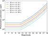 |
Fig. 1 Expected photometric precision of the ET transit module (comprising six 28 cm wide-field telescopes) as a function of target magnitude. The discontinuity at V ≃ 10.5 reflects the assumed onset of detector saturation for the nominal 10 s exposure time, above which we conservatively adopt a constant precision floor rather than further improvement with stellar brightness. |
2.2 Photodynamical modeling: Star-planet-moon configuration
In our simulations, we modeled three-body systems with the Sun as the typical central star. The host planets were chosen to be either Jupiter-like (gas giants) or Earth-like (terrestrial planets). For the exomoon configurations, we considered three categories of moons:
Actual Solar System satellites, including the Moon and the Galilean moons (Io, Europa, Ganymede, and Callisto);
Earth-like moons, with radii between 1.0 and 1.5 R⊕, adopting a mass–radius relation based on a 33% iron + 67% silicate composition (Earth-like model; Zeng & Sasselov 2013);
Sub-Neptune-sized moons, with radii between 2.0 and 4.0 R⊕, using the empirical mass-radius relation from (Wolfgang et al. 2016).
We deliberately excluded exomoons with radii between 1.5 and 2.0 R⊕, as this range corresponds to the “radius valley” (Fulton et al. 2017; Van Eylen et al. 2018), a region where the observed frequency of planets – and by extension, likely exomoons – dips sharply. This gap separates rocky planets (with radii <1.5 R⊕) from sub-Neptunes (with radii >2.0 R⊕). As a result, our chosen exomoon radius regimes correspond to the two distinct populations on either side of this gap. A summary of the parameter selections for all simulated systems is provided in Table 1.
Before simulating the light curves, we first assessed whether the star-planet-moon systems could sustain long-term orbital stability. Moons that cannot survive for a significant fraction of their planet’s lifetime are unlikely to be detectable. Orbital stability is primarily constrained by the Roche limit (the inner boundary) and the Hill radius (the outer boundary). While these provide first-order constraints, additional system parameters, such as the orbital eccentricity and inclination, also influence the actual stable region. Analytical and numerical studies show that retrograde moons tend to have broader stable orbits, while prograde moons are typically confined to orbits within 40% of the Hill radius (Rosario-Franco et al. 2020). Consequently, we adopted 0.4 times the Hill radius as a conservative upper limit for prograde satellite orbits during our simulation.
Based on the orbital period of the host planet, Pb, we classified the planetary systems into two distinct regimes: systems with Pb > 100 d were designated as cold planets, while those with Pb ≤ 100 d were categorized as warm planets. Given ET’s four-year nominal observational baseline, the barycentric orbital periods, Pb, are sampled between 30 and 365 days, while the moon’s orbital periods, Pm, range from 1 to 30 days. To ensure a statistically representative and uniform exploration across these parameter ranges, we constructed a 20 × 20 grid in (log Pm, log Pb) space. This choice ensures a sufficient number of observable transits for robust timing analysis while covering diverse dynamical regimes. For each host-planet configuration, these grid points are further constrained by the Roche limit and 0.4 RHill to guarantee long-term dynamical stability. For every stable pair within the grid, the corresponding semimajor axes (am, ab) are computed via Kepler’s third law. Consequently, no single unique period or semimajor axis is assigned to any system ID; instead, each system comprises an ensemble of discrete orbital realizations sampled from this logarithmic grid.
Table 2 summarizes the adopted orbital parameters for the simulated star-planet-moon systems. These values were selected to represent typical three-body system configurations, ensuring orbital stability while facilitating reproducibility of our simulations.
Parameter selection for the three-body system simulations, categorized based on the choice of the host planet.
2.3 Light curve simulation
Several photodynamical tools have been developed to simulate transit light curves for star-planet-moon systems, including LUNA (Kipping 2011), TLCM (Csizmadia 2020), Gefera (Gordon & Agol 2022), and Pandora (Hippke & Heller 2022). In this study, we adopted Pandora due to its ability to fully account for three-body gravitational interactions and generate synthetic light curves with high fidelity.
Figure 2 presents a representative example from our simulations, showing the light curve of a single transit event from a system with a Jupiter-sized planet on a 30-day orbital period and a 3 R⊕ exomoon on a 1-day orbital period (system ID: simu 21). The light curve exhibits characteristic shadowing modulations caused by the moon’s orbital motion around the planet. This example highlights how Pandora generates detailed transit signatures, which are used as input data for our subsequent analysis of exomoon detectability.
Adopted orbital parameters for the simulated star-planet-moon systems.
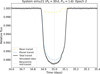 |
Fig. 2 Example of a synthetic light curve generated with Pandora. The shown system (system ID: simu 21) consists of a Jupiter-sized planet with a 30-day orbital period and a 3 R⊕ exomoon on a 1-day orbital period. The simulation assumes a target star with 6 ≤ mV ≤ 10.5 and white Gaussian noise of 138 ppm per 2-minute cadence. The plot displays the flux variation during one planetary transit event, clearly showing the modulation induced by the moon’s orbit. |
3 Detection method
In this section, we describe the methodology for extracting transit variation signals (T×Vs, such as TTVs, TRVs, TDVs, etc.) and evaluating exomoon detectability using these signals.
3.1 T×Vs from light-curve analysis
For each simulated system, we generated noisy transit light curves using Pandora and divided them into individual planet transit epochs. The light curve noise is modeled as stationary white Gaussian noise, with amplitudes scaled to match the expected photometric performance of ET as described in Sect. 2.1. Specifically, we evaluated four representative noise levels: 138 ppm and 88 ppm per cadence for bright targets (6 ≤ V ≤ 10.5) with 2-minute and 5-minute exposures, respectively, and 620 ppm and 392 ppm per cadence for fainter targets (V = 13.5) with 2-minute and 5-minute exposures, respectively. Each simulated system was therefore evaluated under observational conditions spanning ET’s full photometric capability range. We emphasize that our noise model primarily accounts for photon-counting (Poisson) noise, implemented as additive white Gaussian noise via the built-in functionality of Pandora. This approach, however, neglects complex noise sources inherent to real space missions, such as stellar activity (e.g., spots and flares), instrumental systematics, and other unmodeled factors. Consequently, the resulting exomoon detectability should be interpreted as best-case performance under ideal, well-behaved noise conditions, providing a theoretical upper limit for ET’s exomoon sensitivity.
Each epoch was then analyzed using the Transit Analysis module of PyTransit (Parviainen 2015). PyTransit uses the Mandel-Agol model to fit transit light curves, combining global optimization with Markov Chain Monte Carlo (MCMC) sampling to obtain robust posterior distributions of stellar and orbital parameters. In this analysis, we fit each transit epoch (whether or not the system includes a moon) using a single-planet model. Figure 3 presents the light curve fitting for the second transit epoch (Epoch 2) of the representative system simu 21 (Pb = 30 d, Pm= 1 d). The simulated data, which include the exomoon perturbation, are fitted using a planet-only model in PyTransit. The corresponding corner plot from the MCMC fitting of this transit event is shown in Figure 4.
This consistent fitting approach enables us to quantify the differences arising from the presence of an exomoon (in the three-body simulations) versus its absence (as in the two-body simulations). The following key transit-shape parameters were extracted from the light curve fitting for each epoch:
tc : mid-transit time (photometric transit center)
k2 : transit depth
tT : total transit duration (first to fourth contact)
tF : flat-bottomed transit duration (second to third contact)
b : impact parameter
Epoch-to-epoch variations of these parameters define the T×V series: TTVs, TRVs, TDVs, flat-bottomed transit duration variations (TFVs), and impact parameter variations (TbVs). These signals provide the basis for detecting dynamical perturbations induced by potential exomoons.
3.2 Exomoon detectability criteria
We employed a hypothesis-testing framework to distinguish between two-body (planet-only) and three-body (planet-moon) systems – specifically, between simulated two-body and three-body configurations. The core idea was to compare the observed parameter variance in the three-body simulations (var3) against the expected noise distribution derived from two-body simulations (var2).
For the three-body simulations (star-planet-moon), we calculated var3 as the residual variance of the fitted transit parameters. For the mid-transit time (tc), linear trends are first removed via regression (tc = t0 + P • epoch), and then var3, which quantifies scattering in the residual, is calculated as,
 (1)
(1)
where N is the number of epochs (transit events), tci denotes the mid-transit time extracted from the simulated three-body light curve (for epoch i), and  is the predicted mid-transit time from the linear regression model fitted to these tci values. The denominator (N – 2) corrects for two degrees of freedom lost to estimating the regression parameters: t0 (initial mid-transit time) and P (orbital period).
For other transit parameters – including k2, tT, tF, and b – var3 uses one degree of freedom (due to mean subtraction),
 (2)
(2)
where pi denotes the value of the transit parameter extracted from the simulated three-body light curve at epoch i, and  is the mean of these parameter values across all epochs.
To estimate the noise floor in the absence of an exomoon, we generated synthetic variance values (var2) through Monte Carlo bootstrap (MCB) resampling of two-body simulations. For each parameter, the following steps were performed:
Fit the simulated two-body light curves (star-planet only) with a single-planet model using PyTransit’s MCMC sampler, yielding parameter values (pi) and their 1σ uncertainties (σp,i) for each epoch i. Here, σp,i corresponds to the standard deviation of the posterior distribution for parameter p at epoch i, as output by the MCMC chain.
Resample nboot = 5000 synthetic parameter series by adding Gaussian noise to the grand mean of all epoch parameters (
 with N epochs):
  , where ϵi ~ 𝒩(0, σp,i).
For each synthetic series, compute var2 using the same formula as var3 (matching degrees of freedom for consistency).
This process produced a distribution of var2 values, representing the expected variance due to measurement noise alone. An exomoon (extra-body) detection is claimed in the planetary system if var3 exceeds the 99.7th percentile of this distribution. For 5000 bootstrap samples, this threshold corresponds to the 15th largest value (5000 × 0.003 = 15), corresponding to a false positive rate of approximately 0.3%, which aligns with a 3σ significance level in Gaussian statistics. This approach ensures robust rejection of noise-induced false positives.
To quantify the global yield of our simulations, we defined the detection rate as the ratio of the number of systems identified as exomoon candidates (satisfying the 3σ threshold above) to the total number of dynamically stable systems within a given orbital configuration. For example, the warm detection rate was calculated by dividing the number of exomoon candidates detected in warm planetary systems by the total number of simulated warm systems, rather than by all systems combined. This ensures that the detection rate accurately reflects the detectability within the specific parameter regime under consideration, accounting for the unique characteristics of cold and warm planets.
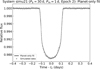 |
Fig. 3 Light curve fitting analysis for the second transit epoch (Epoch 2) of system simu 21. The system consists of a Jupiter-sized planet with a 30-day orbital period and a 3 R⊕ exomoon on a 1-day orbital period. The gray points represent the synthetic photometric data generated by Pandora, which includes the perturbation from a 3 R⊕ exomoon. The solid line indicates the best-fit planet-only model derived from PyTransit. |
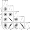 |
Fig. 4 Corner plot derived from the MCMC fitting of the second transit epoch (Epoch 2) of system simu 21. The system parameters are Pb = 30 d and Pm = 1 d. Parameters shown are mid-transit time (tc), transit depth (k2), total transit duration(fT), flat-bottomed transit duration(tF), and impact parameter (b). |
4 Results
In this section, we present the exomoon detection performance of the ET mission across different planetary systems and observing strategies. It is important to emphasize that the results presented herein are derived under the assumption of idealized, white-noise dominated photometry. As discussed in Sect. 3.1, our simulations do not account for time-correlated noise sources, including stellar variability (e.g., spots, flares), instrumental systematics, and other astrophysical or technical noise contributions. Consequently, the detection rates and sensitivity limits reported in the following subsections represent the theoretical baseline performance of the mission in the photon-noise limited regime. Real-world detection efficiencies may be lower depending on the severity of systematic effects, stellar activity levels, and other unmodeled factors.
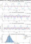 |
Fig. 5 Extracted parameter variation series and MCB detection analysis for system simu 21 (Pm = 1.196 d, Pb = 30 d) over a four-year baseline (49 epochs), (a–c) Residual series for the mid-transit time (tc,TTV), total transit duration (tT, TDV), and flat-bottom duration (tF, TFV). The vertical axes display the deviations in minutes (for tc and tT) or the residual value (for tF). Blue dots connected by solid lines represent the T×Vs from the three-body simulation, exhibiting clear periodic modulations induced by the presence of exomoon. Gray dots represent 100 random T×V series generated from the two-body MCB resamples. The red dashed line denotes zero variation, (d) Histogram of 5000 var2 values (variance of the two-body residuals for tF) with a Gaussian fit (red curve). The vertical solid blue line indicates the observed variance (var3) from the three-body simulation, which lies far beyond the 99.7th percentile threshold (orange dashed line), confirming a robust detection. Black dotted and green dash-dotted lines denote the mean and median of the distribution, respectively. |
4.1 Illustrative case and benchmark analysis
We begin by demonstrating the detection procedure on a specific case study. Figure 5 presents the extracted parameter variation series and the corresponding detection analysis for a 3 R⊕ sub-Neptune-sized exomoon in system simu 21 (Pm = 1.196 d, Pb = 30 d). This simulation covers a four-year observational baseline, resulting in 49 planetary transit epochs.
Panels a through c display the simulated T×V series, including TTV (O – C), TDV (ΔtT), and TFV (ΔtF) respectively. The blue dots and connecting lines represent the T×Vs derived from the three-body simulation (with exomoon), while the gray dots show only 100 T×V series randomly generated from two-body model (without exomoon). Notably, despite the geometric cancellation effects often associated with exomoons (Rodenbeck et al. 2020), panels a and b reveal clear quasi-periodic structures in the TTV and TDV series, confirming that the dynamical signal is preserved and recoverable. For the formal detection criterion, we focus on the tF parameter shown in panel c. As illustrated in the histogram in panel d, the residual variance of tF from the three-body simulation (denoted as var3, vertical blue line) significantly exceeds the 99.7% threshold derived from the null hypothesis distribution (orange dashed line), thereby successfully flagging the detection of an exomoon candidate.
To further explore detectability trends, we evaluated three benchmark systems spanning different exomoon sizes, with the detection maps summarized in Figures 6–8. It is important to note that the detection maps may occasionally display isolated non-detections within otherwise well-detected regions. These irregularities are most likely not physically meaningful but instead reflect stochastic noise realizations, minor fitting uncertainties, or the sensitivity of the adopted 3cr detection threshold. Therefore, the maps are best interpreted statistically, emphasizing overall trends rather than individual outliers.
The key detectability patterns for the star-planet-moon system are summarized as follows:
Moon-sized exomoon (simu 7): Signals are extremely weak. Only one system is flagged as a candidate via the tT parameter (TDVs method), with its var3 barely exceeding the 3σ threshold. No significant signals are detected for other parameters;
Earth-sized exomoon (simu 11): Signals strengthen notably. Over half of the three-body systems are identified as candidates via the tc parameter (TTVs method). In contrast, detectability via other parameters remains limited: no candidates are found using the impact parameter b (TbVs method), with only sporadic detections for the remaining parameters;
3 R⊕ sub-Neptune-sized exomoon (simu 21): Detections are widespread, with recognition rates exceeding 60% for all five parameters. The TTVs (via tc) and TDVs (via tT) methods stand out, exhibiting significantly higher performance than the others.
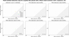 |
Fig. 6 Detection map for a Jupiter-like planet hosting a Moon-sized exomoon (system ID: simu 7), simulated with 120 s exposures and evaluated using a 3σ significance threshold. Gray-shaded regions denote dynamically unstable configurations (within the Roche limit or beyond the Hill radius). The map illustrates exomoon detectability across multiple transit parameter diagnostics (TTVs, TRVs, TDVs, TFVs, TbVs). |
4.2 Exomoon detection around Earth-like planets
We begin by conducting a series of tests on Earth-like host planet systems, each with corresponding exomoons, including Moon-like and Galilean-like satellites (simu 1–5), to assess their detectability. In these simulations, the barycentric orbital periods (Pb) range from 30 to 365 days, with moon periods (Pm) spanning 1–30 days. Assuming a 4-year mission baseline, this corresponds to approximately 5–49 transit events per system. Figure 9a illustrates a representative light curve for this scenario, highlighting the shallow transit depth typical of Earth-sized planets. As an illustrative example, we consider the Earth–Moon analog observed with a 120-second exposure cadence. In this case, the expected moon transit depth is (RMoon/R⊙)2 ≈10 ppm, which is significantly lower than the photometric precision of ET (~138 ppm for bright stars at a 120-second exposure). Consequently, the Moon’s transit signal is effectively buried in the light curve noise, making it undetectable with the ET mission.
Our simulations further indicate that the detection rate of exomoons around Earth-like planets is effectively zero, even when employing T×V analysis. This is primarily because the transit depth of an Earth-sized planet itself (~84 ppm) is comparable to or even lower than the nominal photometric noise floor of ET. Under these low signal-to-noise ratio (S/N) conditions, the measurement uncertainties for transit parameters (e.g., tc) become too large and prevent the detection of exomoon signals using T×V signals. Therefore, we focus our subsequent analysis on Jupiter-like host systems, where their deep transits (~1%) allow for the high-precision T×V measurements required to detect exomoons.
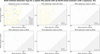 |
Fig. 7 Detection map for a Jupiter-like planet hosting an Earth-sized exomoon (system ID: simu 11), following the same setup as Figure 6 (120 s exposures, 3σ threshold). The map demonstrates the multiparameter T×Vs framework applied to a larger exomoon. |
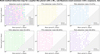 |
Fig. 8 Detection map for a Jupiter-like planet hosting a 3 R⊕ sub-Neptune-sized exomoon (system ID: simu 21), using the same methodology as Figure 6 (120 s exposures, 3σ threshold). Gray-shaded regions indicate dynamically unstable configurations, and the map illustrates the systematic application of T×Vs methods for evaluating larger exomoons with ET-like photometry. |
4.3 Exomoon detection around warm Jupiters
Preliminary tests revealed that Earth-like host systems (simu 1–5) yielded no detectable signals and were thus excluded from further analysis. This left 18 Jupiter-hosted systems (simu 6–23) for detailed investigation. These systems are characterized by short orbital periods (Pb ≈ 30–100 d) and moon periods of 1–12 d. This configuration yields a high number of observable transits, approximately 15 to 49 events over the mission lifetime. A representative transit is shown in Figure 9b, which exhibits a deep (~1%) signal with a relatively short duration. All simulations were conducted using the nominal 120-second cadence of the ET telescope, with results for deeper 300-second exposures discussed in Sect. 5.1. Two stellar magnitude bins were considered: mV = 6–10.5 and mV = 13.5, with results for each case presented separately. This subsection focuses on detection of exomoons in warm Jupiter-like planetary systems, while the detection performance for cold systems is discussed in Sect. 4.4.
Figure 10 summarizes the detection performance of warm Jupiter-like planetary systems at the 3σ significance threshold. As seen from the plot, for bright host stars (mV = 6–10.5; photometric precision ~ 138 ppm), Moon-sized exomoons are effectively undetectable, Earth-sized exomoons are marginally detected by 2–4 methods depending on the system parameters, and sub-Neptune-sized exomoons are easily detectable. For example, more than 93% of candidate systems are identified by at least two methods across the entire simulated sub-Neptune-sized parameter space. For exomoons with radii ≥2.5 R⊕, at least 60% of the stable simulated systems are successfully recognized by all five MCB-based methods. In contrast, for faint host stars (mV = 13.5; photometric precision ~620 ppm), detection rates are lower. Only about 70% of sub-Neptune-sized exomoons are detected by a single method, and none are detected by all five methods.
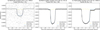 |
Fig. 9 Example transit light curves for the three test cases simulated in this work, (a) An Earth-like planet (Sect. 4.2) showing a shallow transit depth (~100 ppm). We selected Transit #10 from a median system configuration with Pm ≈ 6 d and Pb ≈ 98 d (system ID: simu 2). (b) A warm Jupiter (Sect. 4.3) showing a deep transit with short duration. We selected Transit #17 from a representative system with Pm ≈ 3 d and Pb ≈ 51 d (system ID: simu 20). (c) A cold Jupiter (Sect. 4.4) exhibiting a significantly wider transit duration due to the wider orbit. We selected Transit #5 from a system with Pm ≈ 5 d and Pb ≈ 246 d (system ID: simu 22). The solid black line represents the total flux model, while the gray points show the simulated data with noise. The approximate number of observable transits (Ntr) for each scenario over the 4-year mission baseline is indicated in each panel. |
4.4 Exomoon detection around cold Jupiters
Following the analysis of warm Jupiter-like planetary systems, we now examine the detection performance for cold Jupiter-like systems, adopting the same modeling framework and parameter grid described in Sect. 4.3. These systems correspond to planetary orbital periods Pb spanning 100 to 365 days (with Pm ranging from 1 to 30 days). Due to the wider orbits, the number of transits is lower, ranging from approximately 5 to 14 events, but the transit duration is significantly longer. Figure 9c demonstrates this effect, where the wider transit shape reflects the slower orbital velocity at larger semimajor axes. All other settings (cadence, photometric precision, and significance threshold) remain unchanged. Figure 11 summarizes the detection performance at the 3σ threshold for both bright (mV = 6–10.5; photometric precision ~ 138 ppm) and faint (mV = 13.5; photometric precision ~ 620 ppm) host stars.
Overall, the detection rate exhibits a similar increasing trend with exomoon radius as seen in the warm systems, though with generally lower absolute values. For bright host stars, Moon-sized exomoons remain undetectable, while Earth-sized exomoons show irregular detection rate variations, where it fluctuates non-monotonically with radius. This behavior, consistent with the findings discussed in Sect. 3.2, is most likely due to stochastic noise, fitting uncertainties, or the sensitivity of the adopted 3σ threshold. While minor physical or numerical effects cannot be fully excluded, stochastic noise and uncertainties remain the most likely explanations.
For sub-Neptune-sized exomoons, detection remains relatively efficient, although the completeness is lower compared to the warm regime. Across the parameter space, fewer than 80% of stable systems are identified by at least one detection method. This reduction can be attributed to orbital geometry effects: within the dynamically stable region, systems with larger moon orbital periods are often associated with longer planetary periods, which tend to yield weaker or undetectable combined transit signals. These systems, which are included in the overall cold sample, can reduce the mean detection rate.
For faint host stars, detection performance declines further. Sparse detections are observed, mainly for sub-Neptune-sized exomoons and a few Earth-sized configurations. Most of these detections are flagged by a single method, predominantly TTVs, and systems detected by multiple methods are rare.
4.5 Comparative performance of transit variation metrics
Synthesizing the results from the warm (Sect. 4.3) and cold (Sect. 4.4) Jupiter regimes, we identify a clear and consistent ordering of the five detection methods from most to least efficient: TTVs > TDVs > TRVs > TFVs ≈ TbVs. TTVs exhibit the highest sensitivity across all orbital configurations, particularly for large exomoons with short orbital period. This dominance arises because TTVs directly probe the combined effect of barycentric and photometric contributions from the moon (Szabó et al. 2006). The two effects tend to cancel each other for small high density exomoons (Rodenbeck et al. 2020). However, for close-in large exomoons, the photometric contributions produce coherent and large-amplitude timing shifts that are robustly measurable with high precision photometry data. TDVs rank second, reflecting their shared origin with TTVs, with somewhat reduced amplitude. TRVs primarily trace apparent radius changes induced by overlapping planet-moon transits. TFVs and TbVs show the lowest detection rates; however, they occasionally identify systems missed by higher-ranked methods, underscoring their value as complementary diagnostics.
Detection efficiencies are systematically lower in the cold Jupiter regime compared to warm systems. This reduction primarily reflects the decreased number of observable transits for longer-period planets, rather than an intrinsic degradation of per-transit sensitivity. Notably, the qualitative dependence on exomoon size and the method ranking remain the same across regimes, reinforcing the robustness of our detection framework.
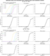 |
Fig. 10 Detection rates for warm Jupiter-like planetary systems at the 3σ significance threshold (120 s cadence), derived from all simulated three-body systems. Top panels a: systems with bright host stars (mV = 6–10.5; photometric precision ~ 138 ppm). Bottom panels b: systems with faint host stars (mV = 13.5; photometric precision ~620 ppm). In each case, the top-left panel shows the fraction of systems identified as potential exomoon candidates by at least n methods (n = 1–5) as a function of exomoon radius. The other panels present the detection rates of five individual MCB-based methods (TTVs, TRVs, TDVs, TFVs, TbVs). Note that in all panels, the detection rate is plotted against the exomoon radius on a logarithmic scale. |
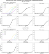 |
Fig. 11 Detection rates for cold Jupiter-like planetary systems at the 3σ significance threshold (120 s cadence), derived from all simulated three-body systems. Top panels a: systems with bright host stars (mV = 6–10.5; photometric precision ~138 ppm). Bottom panels b: systems with faint host stars (mV = 13.5; photometric precision ~620 ppm). In each case, the top-left panel shows the fraction of systems identified as potential exomoon candidates by at least n methods (n = 1–5) as a function of exomoon radius. The other panels present the detection rates of five individual MCB-based methods (TTVs, TRVs, TDVs, TFVs, TbVs). Note that in all panels, the detection rate is plotted against the exomoon radius on a logarithmic scale. |
4.6 Prospects for detecting analogs of the Kepler-1625 b and Kepler-1708 b exomoon candidates
Given the historical importance of the Kepler mission, it is natural to examine whether ET would be capable of detecting exomoon candidates similar to these identified by Kepler. Among all claimed exomoon candidates from Kepler, the most widely discussed ones are the exomoon candidate associated with Kepler-1625 b (Teachey & Kipping 2018; Hamers & Portegies Zwart 2018; Heller et al. 2019; Kreidberg et al. 2019; Teachey et al. 2020; Heller & Hippke 2024; Patel et al. 2025; Kipping et al. 2025) and the exomoon candidate orbiting Kepler-1708 b (Kipping et al. 2022; Cassese & Kipping 2022; Heller & Hippke 2024; Patel et al. 2025; Kipping et al. 2025). For the former, Kepler-1625 b is a Jupiter-sized planet, likely a few times the mass of Jupiter, orbiting a roughly solar-mass star at ~ 1 AU.
The proposed moon, with a radius of ≃4 R⊕ and a mass consistent with a Neptune-like composition, is inferred to orbit at ~40 planetary radii-well inside the planet’s Hill sphere (~200PP). The Kepler-1708 b system hosts another Neptune-sized exomoon candidate. This candidate, with a radius of ≈2.6 R⊕, is inferred to reside at ≈12 planetary radii in an approximately coplanar configuration. The host planet itself is a long-period gas giant orbiting at ~ 1.6 AU from a Sun-like star.
To assess ET’s capability to detect exomoon candidates analogous to those around Kepler-1625 b and Kepler-1708 b, we conducted simulation studies using two different observing baselines: a nominal 4-year mission and an extended 8-year mission scenario, both using the optimal exposure cadence of 120 s. For each simulation, the full MCB-based diagnostic pipeline (TTVs, TDVs, TRVs, TFVs, TbVs) was applied, and detection significance was evaluated following the 3σ statistical framework introduced in Sect. 3.2. The host stars of Kepler-1625 b and Kepler-1708 b have Kepler magnitudes of 15.75 and 15.72, respectively, which are too faint for ET to detect the two exomoon candidates with meaningful significance. We therefore generated a suite of system analogs (hereafter referred to as Kepler-1625 b-like and Kepler-1708 b-like exomoon candidates) by retaining the orbital and physical parameters of the planets and moons, but placing them around brighter host stars with magnitudes mV = 10, 11, 12, 13, and 14.
First, we simulated the Kepler-1625 b-like exomoon candidates using the linear-model system parameters listed in Table 2 of Teachey & Kipping (2018). Under our adopted system configuration, the 4-year and 8-year observing time baselines cover 6 and 11 transit epochs, respectively, given the ~287 day orbital period of Kepler-1625 b. Our results show that, except for the exomoon candidates in the 4-year mission cases with mV = 13 and 14, which are undetected by any of the T×V methods, we are able to detect all remaining simulated exomoon candidates in both the 4-year (mV = 10/11/12) and 8-year (mV = 10/11/12/13/14) mission cases through the TTV method.
Secondly, we simulated the Kepler-1708 b system using the orbital and physical parameters reported in Table 1 of Kipping et al. (2022). Owing to its long orbital period (~737 days), only two transit epochs were observable within a 4-year mission time baseline. As a result, we excluded this scenario from our analysis due to the limited data. Under an 8-year mission baseline, four transit epochs become available. Our simulations show that the exomoon candidates can be identified in at least two TxVs methods for bright host stars, consistent with the detection sensitivity trends found in our earlier simulations. However, the detectability of the TFVs method in the mV = 11 case and the TDVs method in the mV = 12/13 cases remains uncertain, due to the stochastic nature of the simulation.
The simulated prospects for detecting analogs of the Kepler-1625 b and Kepler-1708 b exomoon candidates with the ET mission are summarized in Table 3. In this table, we list the specific methods (among TTVs, TDVs, TRVs, TFVs, and TbVs) that successfully recovered the exomoon signal with a significance greater than 3σ. Our results indicate that the nominal 4-year ET mission has the potential to detect Kepler-1625 b-like exomoon candidates around relatively bright stars using T×V methods, while Kepler-1708 b-like exomoon candidates are likely to remain undetectable.
Detection prospects for Kepler-1625 b-like and Kepler-1708 b-like exomoon candidates with the ET mission.
5 Discussion
5.1 Exomoon detection with different exposure cadence
To identify the optimal observational strategy for detecting exomoon candidates with the ET mission, we compare detection rates obtained under two different exposure cadences: 120 s and 300 s. This comparison focuses on bright host stars (mV = 6-10.5) and faint host stars (mV = 13.5) to evaluate how each exposure setting impacts exomoon detectability.
Figure 12 presents the 3σ detection performance for both warm and cold Jupiter-like planetary systems under 120 s and 300 s exposure cadences, showing results for two stellar brightness regimes (mV = 6-10.5 and mV = 13.5). For single-method detections (n = 1), the sensitivity is comparable between the two exposure durations. However, when multiple detection methods are applied (n ≥ 2), the 120 s exposure consistently outperforms the 300 s exposure, especially for Earth- and sub-Neptune-sized exomoons. In contrast, Moon- and Galilean-like exomoons remain largely undetectable regardless of the exposure cadence.
These results indicate that a 120 s exposure cadence is amore effective strategy for detecting exomoons with the ET mission. From an information-theoretic perspective, shorter cadences always yield superior S/N for transit model fitting (Kipping 2010), despite with reduced photometric precision per exposure. However, the ET mission faces strict constraints on onboard data storage and downlink bandwidth: the 550 square degree field of view and continuous 4-year baseline observation generate data volumes that preclude cadences significantly shorter than 120-s for the primary survey. Within these practical limits, the 120-s mode preserves more dynamical information than the 300-s mode, albeit with reduced photons per exposure. For stars with newly identified exoplanet candidates, we recommend prioritizing the 120-s mode as the finest practical sampling rate, rather than defaulting to longer exposures that would degrade TTV/TDV sensitivity through temporal smearing. This improves the detectability of exomoons, particularly those in the Earth- and sub-Neptune-sized categories.
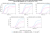 |
Fig. 12 Comparison of 3σ exomoon detection rates in warm (blue) and cold (pink) planetary systems for 120 s (solid lines) and 300 s (dashed lines) exposure cadence. Each panel corresponds to a different minimum number of confirming methods (n ≥ 1 to n ≥ 5), with detection rates shown as a function of exomoon radius. Results are presented for two stellar magnitude ranges: mV = 6–10.5, represented by solid-colored lines, and mV = 13.5, represented by faded lines. |
5.2 Contamination from other effects
The five different transit parameter based methods discussed in this study (TTV, TDV, TRV, TFV, and TbV) exhibit a clear sensitivity hierarchy, among which TTV is the most sensitivity one. However, a statistically significant TTV signal alone is not sufficient, as many unrelated processes can produce contaminating TTV signals. Next we discuss possible contamination sources for TTVs from additional planet in the same system, stellar activity, and secular dynamical effects.
Additional planets represent the primary confusion source. Planet-planet interactions can generate TTVs comparable in amplitude to exomoon-induced signals, especially near mean-motion resonances. However, their characteristic timescales differ significantly. Resonant TTVs oscillate on a super-period (Pj) determined by the distance from resonance,
 (3)
(3)
where P and P′ are the periods of the inner and outer planets, respectively (Lithwick et al. 2012). This super-period depends on the proximity to resonance and is generally tens to hundreds of times longer than the planetary orbital period. In contrast, exomoons must reside within the planetary Hill radius to remain dynamically stable, constraining their orbital periods to be much shorter than that of the host planet. In this work, we consider exomoon configurations with orbital periods spanning approximately 0.003–0.12 × Pplanet. Moreover, planetary perturbations generally lack the accompanying TDV signals characteristic of exomoons, and high precision radial velocity follow-up ata can also be applied to rule out additional planets in the system.
Stellar activity is another significant contaminant (Apai et al. 2018). Starspots and faculae can distort transit shapes and shift best-fitted mid-transit times, introducing apparent TTVs at the stellar rotation period. Although these effects are typically small, they can complicate the interpretation of weak exomoon signals (Ioannidis et al. 2016). Diagnostics for identifying stellar activity include inspecting transit morphology and using multi-wavelength photometry, as spot-induced distortions are strongly chromatic whereas dynamical signals from exomoons are not.
Secular dynamical effects, primarily including tidal orbital decay, apsidal precession, and light-travel time effects induced by wide companions, can introduce TTVs, yet their distinct timescales distinguish them from exomoon signals. Tidal orbital decay produces a monotonie, quadratically growing timing offset that is typically limited to tens of seconds over a long time base-line(tens of years), reaching ~1–3 minutes only in rare extreme systems (e.g., WASP-12 b; (Patra et al. 2017; Maciejewski et al. 2018; Turner et al. 2021; Wang et al. 2024)). Apsidal precession, driven by tidal bulges and general relativity, generates long-term periodic TTVs (Miralda-Escudé 2002; Heyl & Gladman 2007; Ragozzine & Wolf 2009). Importantly, without extended observational baselines or secondary eclipse data, the signal from apsidal precession can be difficult to distinguish from orbital decay (Yee et al. 2020; Barker et al. 2024; Biswas et al. 2024; Winn & Stefánsson 2025). Light-travel time signals similarly evolve on timescale from years to tens of years (Borkovits et al. 2015). Generally, these slowly varying or monotonie signals, together with the lack of accompanying TDV signals, are readily distinguishable from the short-period, high-frequency phase-coherent TTVs expected from close-in exomoon perturbations.
Instrumental and observational systematics (pointing jitter, detector behavior, thermal drifts) may introduce additional timing or depth fluctuations. Although largely mitigable through detrending and cross-validation methods, their contributions should be assessed carefully when evaluating exomoon candidates.
In the purely dynamical limit, exomoon-induced TTVs and TDVs are expected to exhibit a strict π/2 phase offset, with TDVs lagging TTVs by one quarter of the moon’s orbital period (Kipping 2009a; Heller et al. 2016). However, recent studies demonstrate that this relationship is often more complex in realistic observing scenarios. As shown by Rodenbeck et al. (2020), the interplay between the dynamical (barycentric) motion and the photometric (geometric) distortion can alter the shape and phase of the variations in transit timing and duration. Consequently, a strict phase offset of π/2 may not always be observable, particularly for short-period large exomoons where photometric effects dominate. Therefore, a robust exomoon detection should satisfy the following validation criteria: (1) a statistically significant TTV signal exceeding the 3σ threshold; (2) evidence of coupled quasi-periodic variability in both of the TTV and TDV series which indicates a common source, even if the phase relationship is distorted; (3) consistency with other photometric indicators, such as apparent TRVs as suggested by Rodenbeck et al. (2020); and (4) statistically significant preference for a planet-moon dynamical model over competing explanations, including planetary perturbations or stellar activity, using transit-folding technique (Kipping 2021). Satisfying these criteria collectively, rather than relying on phase coherence alone, provides reliable discrimination between genuine exomoon signatures and astrophysical contaminants.
5.3 Comparison with out-of-planetary-transit folding technique
Alternative techniques have been proposed to detect exomoons that differ from the dynamical TTV/TDV framework employed in this work. Notably, Kipping (2021) proposed a transit-folding algorithm (termed “Transit Origami”) that isolates the photometric signature of the exomoon by masking out the planetary transit and searching only for residual in-transit data from the satellite. This technique was motivated by the recognition that high-cadence photometry from missions such as Kepler enables the identification of fine-scale ingress and egress features that are smeared out in standard folding procedures.
However, Heller & Hippke (2022) demonstrated that this approach incurs a substantial cost for close-in exomoons. Because the transit-folding algorithm discards data points contaminated by the planetary transit, the fraction of usable in-transit data decreases dramatically for close-in exomoons. For an Io-like satellite (Pm ≈1.8 days) orbiting a Jupiter-mass planet, Heller & Hippke (2022) calculated that only ~14% of the total in-transit data remains uncontaminated, reducing the effective S/N to approximately 38% of that achievable with full photodynamical modeling. This data loss penalty is particularly severe for the short-period, large-radius exomoons that our simulations identify as the most detectable population using TTV technique with the ET mission.
The TTV-based detection framework presented in this work exhibits advantages in this close-in exomoon regime, which are directly reflected in our detection map (Figure 8). Rather than relying on the direct photometric signature of the exomoon, TTVs exploit the apparent variations of the mid-transit times of the host planet. For the sub-Neptune-sized exomoon benchmark (simu 21, Pm = 1 day), our TTV method achieves detection efficiencies exceeding 60% for warm and cold Jupiter systems, whereas a folding approach would face severe S/N limitations due to the high probability of planet-moon transit overlap at such short orbital separations. Similarly, for Earth-sized satellites (simu 11), the TTV method recovers >50% of warm systems, while folding algorithms would be restricted to a small subset of transits with favorable geometric configurations.
It is important to emphasize that these methods are complementary rather than competing. The transit-folding technique retains advantages for wide-separation satellites, where the geometric probability of overlapping transits is low and the satellite’s direct photometric signal may be resolvable without dynamical modeling (Heller & Hippke 2022). Conversely, TTVs excel for dynamically hot, close-in satellite populations. The ET mission’s high photometric precision and flexible cadence mode enable the application of both techniques, and a combined analysis – searching for phase-coherent TTV/TDV signals while independently vetting candidates with folding diagnostics – would provide the most robust path to exomoon validation. The simulated ET dataset that we release can facilitate such future analyses by the broader exoplanet community.
6 Conclusion
In this study, we explored the detectability of exomoons using the ET mission by employing a detailed simulation framework to model a wide range of exomoon systems. By simulating transit light curves for dynamically stable star-planet-moon configurations, we assessed the feasibility of detecting exomoons around both Earth-like and Jupiter-like host planets. Our results demonstrate that while detection of exomoons around Earth-like planets is largely impractical due to the low transit depths relative to ET’s photometric precision, large exomoons orbiting giant planets show promising detection rates.
For bright stars, sub-Neptune-sized exomoons around warm Jupiters are easily detectable, with detection rates exceeding 60% for systems with moon radii ≥2.5 R⊕. Detection is still possible for Earth-sized exomoons, though with lower efficiency, and Moon-sized exomoons are effectively undetectable. The performance drops for faint stars (mV = 13.5), where detection rates are generally lower and primarily limited to sub-Neptune-sized exomoons. Our analysis reveals that the detection performance is strongly influenced by the size of the exomoon, the orbital period of the host planet, and the photometric precision of the observations. The use of multiple detection methods, such as TTVs and TRVs, further enhances the reliability of exomoon identification, underscoring the complementary value of these techniques in identifying exomoons. However, we emphasize that these results are derived under the assumption of stationary white Gaussian noise. As real observations will inevitably be affected by stellar variability, instrumental systematics, and other unmodeled factors, the detection rates reported here represent the theoretical best-case performance of the ET mission.
Overall, this study highlights the potential of the ET mission to detect exomoons around giant planets, such as Kepler-1625 b-like exomoon candidates. These results provide valuable insights into the detection capabilities of space-based high-precision photometric telescopes and contribute to our understanding of exomoon systems, paving the way for future observations and the discovery of exomoons in exoplanetary systems. The simulated ET mission exomoon dataset will also be made publicly available within the community, and can be used for future data challenge study aiming at developing exomoon detection algorithms for the ET mission.
Acknowledgements
We sincerely thank the anonymous referee for the thorough, insightful, and highly constructive comments, which have significantly improved the manuscript. The work was supported by the National Key R&D Program of China (2024YFA1611801), the NSFC grant 12073092, the science research grants from the China Manned Space Project (No. CMS-CSST2025-A16), and the Earth 2.0 Space Mission program from SHAO for their financial support. The ET mission is funded by China’s Space Origins Exploration Program. We also thank the developers of the open-source software packages Pandora and PyTransit for their contributions to the scientific community.
References
- Agol, E., Jansen, T., Lacy, B., Robinson, T. D., & Meadows, V. 2015, ApJ, 812, 5 [NASA ADS] [CrossRef] [Google Scholar]
- Apai, D., Rackham, B. V., Giampapa, M. S., et al. 2018, ARXiv e-prints [arXiv:1803.08708] [Google Scholar]
- Barker, A. J., Efroimsky, M., Makarov, V. V., & Veras, D. 2024, MNRAS, 527, 5131 [Google Scholar]
- Benz, W., Broeg, C., Fortier, A., et al. 2021, Exp. Astron., 51, 109 [Google Scholar]
- Biswas, S., Bisht, D., Jiang, I.-G., Sariya, D. P., & Parthasarathy, K. 2024, AJ, 168, 176 [Google Scholar]
- Borkovits, T., Rappaport, S., Hajdu, T., & Sztakovics, J. 2015, MNRAS, 448, 946 [NASA ADS] [CrossRef] [Google Scholar]
- Borucki, W. J. 2016, Rep. Prog. Phys., 79, 036901 [Google Scholar]
- Borucki, W. J., Koch, D., Basri, G., et al. 2010, Science, 327, 977 [Google Scholar]
- Cassese, B., & Kipping, D. 2022, MNRAS, 516, 3701 [Google Scholar]
- Csizmadia, S. 2020, MNRAS, 496, 4442 [Google Scholar]
- Fox, C., & Wiegert, P. 2021, MNRAS, 501, 2378 [NASA ADS] [CrossRef] [Google Scholar]
- Fulton, B. J., Petigura, E. A., Howard, A. W., et al. 2017, AJ, 154, 109 [Google Scholar]
- Ge, J., Zhang, H., Deng, H., Howell, S. B., & the ET Team 2022a, Innovation, 3, 100271 [Google Scholar]
- Ge, J., Zhang, H., Zang, W., et al. 2022b, ARXiv e-prints [arXiv:2206.06693] [Google Scholar]
- Ge, J., Zhang, H., Zhang, Y., et al. 2022c, SPIE Conf. Ser., 12180, 1218015 [Google Scholar]
- Ge, J., Chen, W., Chen, Y., et al. 2024a, Chinese J. Space Sci., 44, 400 [Google Scholar]
- Ge, J., Zhang, H., Zhang, Y., et al. 2024b, SPIE Conf. Ser., 13092, 1309218 [Google Scholar]
- Gebek, A., & Oza, A. V. 2020, MNRAS, 497, 5271 [Google Scholar]
- Gordon, T. A., & Agol, E. 2022, AJ, 164, 111 [NASA ADS] [CrossRef] [Google Scholar]
- Hamers, A. S., & Portegies Zwart, S. F. 2018, ApJ, 869, L27 [NASA ADS] [CrossRef] [Google Scholar]
- Heller, R., & Hippke, M. 2022, A&A, 657, A119 [NASA ADS] [CrossRef] [EDP Sciences] [Google Scholar]
- Heller, R., & Hippke, M. 2024, Nat. Astron., 8, 193 [Google Scholar]
- Heller, R., Hippke, M., Placek, B., Angerhausen, D., & Agol, E. 2016, A&A, 591, A67 [NASA ADS] [CrossRef] [EDP Sciences] [Google Scholar]
- Heller, R., Rodenbeck, K., & Bruno, G. 2019, A&A, 624, A95 [NASA ADS] [CrossRef] [EDP Sciences] [Google Scholar]
- Heyl, J. S., & Gladman, B. J. 2007, MNRAS, 377, 1511 [NASA ADS] [CrossRef] [Google Scholar]
- Hinkel, N. R., & Kane, S. R. 2013, ApJ, 774, 27 [Google Scholar]
- Hippke, M., & Heller, R. 2022, A&A, 662, A37 [NASA ADS] [CrossRef] [EDP Sciences] [Google Scholar]
- Ioannidis, P., Huber, K. F., & Schmitt, J. H. M. M. 2016, A&A, 585, A72 [NASA ADS] [CrossRef] [EDP Sciences] [Google Scholar]
- Johnson, R. E., & Huggins, P. J. 2006, PASP, 118, 1136 [Google Scholar]
- Kipping, D. M. 2009a, MNRAS, 392, 181 [NASA ADS] [CrossRef] [Google Scholar]
- Kipping, D. M. 2009b, MNRAS, 396, 1797 [NASA ADS] [CrossRef] [Google Scholar]
- Kipping, D. M. 2010, MNRAS, 408, 1758 [Google Scholar]
- Kipping, D. M. 2011, MNRAS, 416, 689 [NASA ADS] [Google Scholar]
- Kipping, D. 2021, MNRAS, 507, 4120 [NASA ADS] [CrossRef] [Google Scholar]
- Kipping, D., & Yahalomi, D. A. 2023, MNRAS, 518, 3482 [Google Scholar]
- Kipping, D. M., Bakos, G. Á., Buchhave, L., Nesvorný, D., & Schmitt, A. 2012, ApJ, 750, 115 [NASA ADS] [CrossRef] [Google Scholar]
- Kipping, D., Bryson, S., Burke, C., et al. 2022, Nat. Astron., 6, 367 [NASA ADS] [CrossRef] [Google Scholar]
- Kipping, D., Teachey, A., Yahalomi, D. A., et al. 2025, Nat. Astron., 9, 795 [Google Scholar]
- Kral, Q., Wang, J., Kammerer, J., et al. 2026, A&A, 705, A217 [NASA ADS] [CrossRef] [EDP Sciences] [Google Scholar]
- Kreidberg, L., Luger, R., & Bedell, M. 2019, ApJ, 877, L15 [NASA ADS] [CrossRef] [Google Scholar]
- Liebig, C., & Wambsganss, J. 2010, A&A, 520, A68 [NASA ADS] [CrossRef] [EDP Sciences] [Google Scholar]
- Limbach, M. A., Vos, J. M., Winn, J. N., et al. 2021, ApJ, 918, L25 [CrossRef] [Google Scholar]
- Lithwick, Y., Xie, J., & Wu, Y. 2012, ApJ, 761, 122 [Google Scholar]
- Ma, X., Wang, W., Zhang, Z., et al. 2025, AJ, 169, 169 [Google Scholar]
- Maciejewski, G., Fernández, M., Aceituno, F., et al. 2018, Acta Astron., 68, 371 [NASA ADS] [Google Scholar]
- Miralda-Escudé, J. 2002, ApJ, 564, 1019 [Google Scholar]
- Miyazaki, S., Sumi, T., Bennett, D. P., et al. 2018, AJ, 156, 136 [Google Scholar]
- Noyola, J. P., Satyal, S., & Musielak, Z. E. 2014, ApJ, 791, 25 [Google Scholar]
- Noyola, J. P., Satyal, S., & Musielak, Z. E. 2016, ApJ, 821, 97 [Google Scholar]
- Oza, A. V., Johnson, R. E., Lellouch, E., et al. 2019, ApJ, 885, 168 [Google Scholar]
- Parviainen, H. 2015, MNRAS, 450, 3233 [Google Scholar]
- Patel, S. D., Quarles, B., & Cuntz, M. 2025, MNRAS, 537, 2291 [Google Scholar]
- Patra, K. C., Winn, J. N., Holman, M. J., et al. 2017, AJ, 154, 4 [Google Scholar]
- Peters-Limbach, M. A., & Turner, E. L. 2013, ApJ, 769, 98 [NASA ADS] [CrossRef] [Google Scholar]
- Ragozzine, D., & Wolf, A. S. 2009, ApJ, 698, 1778 [Google Scholar]
- Rauer, H., Catala, C., Aerts, C., et al. 2014, Exp. Astron., 38, 249 [Google Scholar]
- Ricker, G. R., Winn, J. N., Vanderspek, R., et al. 2015, J. Astron. Telesc. Instrum. Syst., 1, 014003 [Google Scholar]
- Rodenbeck, K., Heller, R., Hippke, M., & Gizon, L. 2018, A&A, 617, A49 [NASA ADS] [CrossRef] [EDP Sciences] [Google Scholar]
- Rodenbeck, K., Heller, R., & Gizon, L. 2020, A&A, 638, A43 [NASA ADS] [CrossRef] [EDP Sciences] [Google Scholar]
- Rosario-Franco, M., Quarles, B., Musielak, Z. E., & Cuntz, M. 2020, AJ, 159, 260 [Google Scholar]
- Ruffio, J.-B., Horstman, K., Mawet, D., et al. 2023, AJ, 165, 113 [NASA ADS] [CrossRef] [Google Scholar]
- Sartoretti, P., & Schneider, J. 1999, A&AS, 134, 553 [Google Scholar]
- Simon, A., Szatmáry, K., & Szabó, G. M. 2007, A&A, 470, 727 [NASA ADS] [CrossRef] [EDP Sciences] [Google Scholar]
- Simon, A. E., Szabó, G. M., Szatmáry, K., & Kiss, L. L. 2010, MNRAS, 406, 2038 [NASA ADS] [Google Scholar]
- Sucerquia, M., Alvarado-Montes, J. A., Bayo, A., et al. 2022, MNRAS, 512, 1032 [NASA ADS] [CrossRef] [Google Scholar]
- Szabó, G. M., Szatmáry, K., Divéki, Z., & Simon, A. 2006, A&A, 450, 395 [NASA ADS] [CrossRef] [EDP Sciences] [Google Scholar]
- Szabó, G. M., Schneider, J., Dencs, Z., & Kálmán, S. 2024, Universe, 10, 110 [Google Scholar]
- Teachey, A., & Kipping, D. M. 2018, Sci. Adv., 4, eaav1784 [Google Scholar]
- Teachey, A., Kipping, D., Burke, C. J., Angus, R., & Howard, A. W. 2020, AJ, 159, 142 [NASA ADS] [CrossRef] [Google Scholar]
- Teachey, A. 2024, ARXiv e-prints [arXiv:2401.13293] [Google Scholar]
- Timmermann, A., Heller, R., Reiners, A., & Zechmeister, M. 2020, A&A, 635, A59 [NASA ADS] [CrossRef] [EDP Sciences] [Google Scholar]
- Turner, J. D., Ridden-Harper, A., & Jayawardhana, R. 2021, AJ, 161, 72 [NASA ADS] [CrossRef] [Google Scholar]
- Van Eylen, V., Agentoft, C., Lundkvist, M. S., et al. 2018, MNRAS, 479, 4786 [Google Scholar]
- Wang, W., Zhang, Z., Chen, Z., et al. 2024, ApJS, 270, 14 [NASA ADS] [CrossRef] [Google Scholar]
- Wang, W., Ma, X., Chen, Z., et al. 2025, ApJ, 986, 121 [Google Scholar]
- Winn, J. N., & Stefánsson, G. 2025, Planet. Sci. J., 6, 300 [Google Scholar]
- Winterhalder, T. O., Mérand, A., Kammerer, J., et al. 2026, A&A, 705, A216 [NASA ADS] [CrossRef] [EDP Sciences] [Google Scholar]
- Wolfgang, A., Rogers, L. A., & Ford, E. B. 2016, ApJ, 825, 19 [Google Scholar]
- Yahalomi, D. A., Kipping, D., Nesvorný, D., et al. 2024, MNRAS, 527, 620 [Google Scholar]
- Yee, S. W., Winn, J. N., Knutson, H. A., et al. 2020, ApJ, 888, L5 [Google Scholar]
- Zeng, L., & Sasselov, D. 2013, PASP, 125, 227 [Google Scholar]
- Zhang, Z., Wang, W., Ma, X., et al. 2024, ApJS, 275, 32 [Google Scholar]
Appendix A Application to real observation data
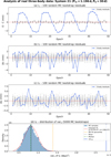 |
Fig. A.1 Same as Fig. 5, but for the real observed three-body light curve analysis. It is clear that we can detect the exomoon candidate here. |
When analyzing “real” light curve from the ET mission, we propose the following practical workflow for exomoon candidate identification:
Fit the light curve. We first fit a standard two-body (planet-only) transit model to the observed light curve to obtain best-fit planetary parameters, including the orbital period P, mid-transit time t0, transit depth k2, impact parameter b, limb-darkening parameters, etc. We calculate varobs following the same procedure described in Eqs. (1) and (2).
Estimate the noise level. We calculate the root-mean-square (RMS) of the flux residuals in the out-of-transit (flat) portions of the light curve to quantify the actual photometric noise level, denoted σobs.
Generate the reference distribution. Using the best-fit two-body model from Step 1 above, we generate one synthetic light curve with white Gaussian photometric noise corresponding to σobs. For this simulated two-body synthetic light curve, we fit a single-planet model using PyTransit to extract transit parameters and their 1er uncertainties. We generate nboot = 5000 synthetic parameter series following the same procedure in Sect. 3.2, and calculate 5000 var2 (planet-only distribution).
Compare and flag candidates. We then compare the variance of the observed data, varobs, against this simulated distribution of var2. If varobs significantly exceeds the median var2 (e.g., > 3σ threshold as shown in Fig. 5), the planetary system is then flagged as an exomoon candidate.
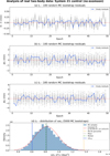 |
Fig. A.2 Same as Fig. 5, but for the real observed two-body light curve analysis. It is clear that we do not detect an exomoon candidate here. |
We applied this proposed workflow to two simulated real light curves from ET mission: one containing an exomoon (the three-body light curve) and one without (the two-body light curve). The results are shown in Fig. A.1 and Fig. A.2. Our tests demonstrate that this practical implementation yields similar detection sensitivity as that obtained in our previous simulations in Sect. 3.2 (see Fig. 5). Thus, this MCB approach provides a robust, data-driven assessment of whether observed transit variations exceed the expected scatter from photometric noise alone, without requiring prior assumptions about the existence of exomoons.
All Tables
Parameter selection for the three-body system simulations, categorized based on the choice of the host planet.
Detection prospects for Kepler-1625 b-like and Kepler-1708 b-like exomoon candidates with the ET mission.
All Figures
|
Fig. 1 Expected photometric precision of the ET transit module (comprising six 28 cm wide-field telescopes) as a function of target magnitude. The discontinuity at V ≃ 10.5 reflects the assumed onset of detector saturation for the nominal 10 s exposure time, above which we conservatively adopt a constant precision floor rather than further improvement with stellar brightness. |
| In the text | |
|
Fig. 2 Example of a synthetic light curve generated with Pandora. The shown system (system ID: simu 21) consists of a Jupiter-sized planet with a 30-day orbital period and a 3 R⊕ exomoon on a 1-day orbital period. The simulation assumes a target star with 6 ≤ mV ≤ 10.5 and white Gaussian noise of 138 ppm per 2-minute cadence. The plot displays the flux variation during one planetary transit event, clearly showing the modulation induced by the moon’s orbit. |
| In the text | |
|
Fig. 3 Light curve fitting analysis for the second transit epoch (Epoch 2) of system simu 21. The system consists of a Jupiter-sized planet with a 30-day orbital period and a 3 R⊕ exomoon on a 1-day orbital period. The gray points represent the synthetic photometric data generated by Pandora, which includes the perturbation from a 3 R⊕ exomoon. The solid line indicates the best-fit planet-only model derived from PyTransit. |
| In the text | |
|
Fig. 4 Corner plot derived from the MCMC fitting of the second transit epoch (Epoch 2) of system simu 21. The system parameters are Pb = 30 d and Pm = 1 d. Parameters shown are mid-transit time (tc), transit depth (k2), total transit duration(fT), flat-bottomed transit duration(tF), and impact parameter (b). |
| In the text | |
|
Fig. 5 Extracted parameter variation series and MCB detection analysis for system simu 21 (Pm = 1.196 d, Pb = 30 d) over a four-year baseline (49 epochs), (a–c) Residual series for the mid-transit time (tc,TTV), total transit duration (tT, TDV), and flat-bottom duration (tF, TFV). The vertical axes display the deviations in minutes (for tc and tT) or the residual value (for tF). Blue dots connected by solid lines represent the T×Vs from the three-body simulation, exhibiting clear periodic modulations induced by the presence of exomoon. Gray dots represent 100 random T×V series generated from the two-body MCB resamples. The red dashed line denotes zero variation, (d) Histogram of 5000 var2 values (variance of the two-body residuals for tF) with a Gaussian fit (red curve). The vertical solid blue line indicates the observed variance (var3) from the three-body simulation, which lies far beyond the 99.7th percentile threshold (orange dashed line), confirming a robust detection. Black dotted and green dash-dotted lines denote the mean and median of the distribution, respectively. |
| In the text | |
|
Fig. 6 Detection map for a Jupiter-like planet hosting a Moon-sized exomoon (system ID: simu 7), simulated with 120 s exposures and evaluated using a 3σ significance threshold. Gray-shaded regions denote dynamically unstable configurations (within the Roche limit or beyond the Hill radius). The map illustrates exomoon detectability across multiple transit parameter diagnostics (TTVs, TRVs, TDVs, TFVs, TbVs). |
| In the text | |
|
Fig. 7 Detection map for a Jupiter-like planet hosting an Earth-sized exomoon (system ID: simu 11), following the same setup as Figure 6 (120 s exposures, 3σ threshold). The map demonstrates the multiparameter T×Vs framework applied to a larger exomoon. |
| In the text | |
|
Fig. 8 Detection map for a Jupiter-like planet hosting a 3 R⊕ sub-Neptune-sized exomoon (system ID: simu 21), using the same methodology as Figure 6 (120 s exposures, 3σ threshold). Gray-shaded regions indicate dynamically unstable configurations, and the map illustrates the systematic application of T×Vs methods for evaluating larger exomoons with ET-like photometry. |
| In the text | |
|
Fig. 9 Example transit light curves for the three test cases simulated in this work, (a) An Earth-like planet (Sect. 4.2) showing a shallow transit depth (~100 ppm). We selected Transit #10 from a median system configuration with Pm ≈ 6 d and Pb ≈ 98 d (system ID: simu 2). (b) A warm Jupiter (Sect. 4.3) showing a deep transit with short duration. We selected Transit #17 from a representative system with Pm ≈ 3 d and Pb ≈ 51 d (system ID: simu 20). (c) A cold Jupiter (Sect. 4.4) exhibiting a significantly wider transit duration due to the wider orbit. We selected Transit #5 from a system with Pm ≈ 5 d and Pb ≈ 246 d (system ID: simu 22). The solid black line represents the total flux model, while the gray points show the simulated data with noise. The approximate number of observable transits (Ntr) for each scenario over the 4-year mission baseline is indicated in each panel. |
| In the text | |
|
Fig. 10 Detection rates for warm Jupiter-like planetary systems at the 3σ significance threshold (120 s cadence), derived from all simulated three-body systems. Top panels a: systems with bright host stars (mV = 6–10.5; photometric precision ~ 138 ppm). Bottom panels b: systems with faint host stars (mV = 13.5; photometric precision ~620 ppm). In each case, the top-left panel shows the fraction of systems identified as potential exomoon candidates by at least n methods (n = 1–5) as a function of exomoon radius. The other panels present the detection rates of five individual MCB-based methods (TTVs, TRVs, TDVs, TFVs, TbVs). Note that in all panels, the detection rate is plotted against the exomoon radius on a logarithmic scale. |
| In the text | |
|
Fig. 11 Detection rates for cold Jupiter-like planetary systems at the 3σ significance threshold (120 s cadence), derived from all simulated three-body systems. Top panels a: systems with bright host stars (mV = 6–10.5; photometric precision ~138 ppm). Bottom panels b: systems with faint host stars (mV = 13.5; photometric precision ~620 ppm). In each case, the top-left panel shows the fraction of systems identified as potential exomoon candidates by at least n methods (n = 1–5) as a function of exomoon radius. The other panels present the detection rates of five individual MCB-based methods (TTVs, TRVs, TDVs, TFVs, TbVs). Note that in all panels, the detection rate is plotted against the exomoon radius on a logarithmic scale. |
| In the text | |
|
Fig. 12 Comparison of 3σ exomoon detection rates in warm (blue) and cold (pink) planetary systems for 120 s (solid lines) and 300 s (dashed lines) exposure cadence. Each panel corresponds to a different minimum number of confirming methods (n ≥ 1 to n ≥ 5), with detection rates shown as a function of exomoon radius. Results are presented for two stellar magnitude ranges: mV = 6–10.5, represented by solid-colored lines, and mV = 13.5, represented by faded lines. |
| In the text | |
|
Fig. A.1 Same as Fig. 5, but for the real observed three-body light curve analysis. It is clear that we can detect the exomoon candidate here. |
| In the text | |
|
Fig. A.2 Same as Fig. 5, but for the real observed two-body light curve analysis. It is clear that we do not detect an exomoon candidate here. |
| In the text | |
Current usage metrics show cumulative count of Article Views (full-text article views including HTML views, PDF and ePub downloads, according to the available data) and Abstracts Views on Vision4Press platform.
Data correspond to usage on the plateform after 2015. The current usage metrics is available 48-96 hours after online publication and is updated daily on week days.
Initial download of the metrics may take a while.