| Issue |
A&A
Volume 694, February 2025
|
|
|---|---|---|
| Article Number | L8 | |
| Number of page(s) | 7 | |
| Section | Letters to the Editor | |
| DOI | https://doi.org/10.1051/0004-6361/202452968 | |
| Published online | 07 February 2025 | |
Letter to the Editor
Extreme exomoons in WASP-49 Ab: Dynamics and detectability
Univ. Grenoble Alpes, CNRS, IPAG, 38000 Grenoble, France
⋆ Corresponding author; This email address is being protected from spambots. You need JavaScript enabled to view it.
Received:
12
November
2024
Accepted:
9
January
2025
Abstract
Context. WASP-49Ab, a low-density Saturn-like planet in a tight orbit around a Sun-like star within a wide binary system, is a compelling candidate for hosting a volcanic moon, as suggested by the detection of Doppler-shifted sodium.
Aims. This study evaluates the stability of potential satellites around WASP-49Ab under the influence of planetary oblateness, relativistic effects, and perturbations from a close companion star, focusing on their impact on light curve parameters such as transit duration and impact parameter variations, driven by the evolution of the planet’s orbit in this extreme environment.
Methods. Using N-body simulations and semi-analytical methods, we analysed moon’s dynamics across varied initial conditions and gravitational frameworks including the potential of an oblate planet and the effects of the general relativity.
Results. We find that ‘selenity’, a moon survival indicator, is high in close orbits with low eccentricity and near the Roche limit, especially for masses higher than Io’s. Stability decreases as eccentricity or distance from the planet increases. Additionally, we observe a strong destabilising resonance near 1.4 Rp when planetary eccentricities are considered to be ≳0.
Conclusions. This study confirms the potential for stable exomoons around WASP-49Ab despite its hostile environment, emphasising the importance of incorporating diverse physical effects in stability analyses, aiding future detection efforts.
Key words: planets and satellites: detection / planets and satellites: dynamical evolution and stability / stars: individual: WASP-49
© The Authors 2025
 Open Access article, published by EDP Sciences, under the terms of the Creative Commons Attribution License (https://creativecommons.org/licenses/by/4.0), which permits unrestricted use, distribution, and reproduction in any medium, provided the original work is properly cited.
This article is published in open access under the Subscribe to Open model. This email address is being protected from spambots. You need JavaScript enabled to view it. to support open access publication.
1. Introduction
According to formation models (Canup & Ward 2006), moons are anticipated to be common around Jupiter-like planets. Given the prevalence of these planets, the successful detection or absence of exomoons would have significant implications for current models of planetary migration and lunar habitability (Barnes & O’Brien 2002; Sucerquia et al. 2019; Martínez-Rodríguez et al. 2019; Sucerquia et al. 2020).
Direct exomoon detection is challenging due to limited resolution and sensitivity to weak signals from small nearby moons. A promising alternative is analysing light curve variations during planetary transits. These variations include transit timing variations (TTVs, Kipping 2009a), transit duration variations (TDVs, Kipping 2009b), and transit radius variations (TRVs, Rodenbeck et al. 2020), which can provide insights into the presence of moons or nearby planets. While difficult to detect, these secondary effects currently represent some of the most effective techniques for revealing the presence of undiscovered moons.
The search for exomoons has gained significant interest, particularly with candidates like Kepler-1625b-i, a Neptune-sized moon orbiting a super-Jovian planet, and Kepler-1708b-i, approximately 2.6 Earth radii, orbiting its Jupiter-sized host at 12 planetary radii. Kepler-1625b-i was proposed through mutual transits of the planet and moon (Teachey & Kipping 2018), while Kepler-1708b-i emerged from a survey of 70 cool giant exoplanets (Kipping et al. 2022). However, these findings are debated due to uncertainties in the physical and orbital characteristics of these systems (Kreidberg et al. 2019). The significant high planet-to-moon ratio of these candidates challenges traditional moon formation models, such as accretion capture, suggesting a new class of gas giant moons (Heller 2018; Teachey & Kipping 2018) or even ringed moons (Sucerquia et al. 2022).
An alternative approach to exomoon detection focuses on the activity within planetary environments. Stellar winds can erode nearby moons, producing halos of material, or tidal dynamics can expel particles, creating detectable photometric signatures around planets with moons. This is the case with the WASP-49Ab system (Lendl et al. 2012), a Saturn-like planet in a 2.8-day S-type orbit around a Sun-like star within a binary system, where neutral sodium (Na I) has been detected in the planetary atmosphere (Oza et al. 2024). The detection of this alkali metal, with notable night-to-night variations in spectral flux, suggests the possible existence of an external source, such as a volcanic exomoon, akin to Jupiter’s Io. Observations with the Echelle SPectrograph for Rocky Exoplanets and Stable Spectroscopic Observations (ESPRESSO) reveal a Doppler shift of approximately +9.7 km/s relative to the planet’s reference frame, which could suggest the presence of a satellite orbiting WASP-49Ab.
Potential moons around WASP-49Ab must reside in a narrow region between the Roche limit and the Hill sphere (∼1.2–1.8 planetary radii) to maintain dynamical stability, and to avoid destabilising evection and eviction resonances (Vaillant & Correia 2022). Whilst previous studies have explored individual perturbations, such as tides (Barnes & Fortney 2004; Domingos et al. 2006; Alvarado-Montes et al. 2017) or binary companions (Quarles et al. 2021; Gordon et al. 2024), here we integrate multiple effects including planetary oblateness (Hong et al. 2015) and relativistic corrections, making the inclusion of these under-explored effects pivotal in this extreme environment.
We first describe the WASP-49Ab system in Sect. 2. Then we report our numerical simulations to assess the long-term stability of potential satellites and examine the impact on light curves in Sects. 3 and 4. Finally, we discuss how these perturbations may impact upcoming exomoon detections in Sect. 5.
2. The WASP-49Ab system and perturbative forces
WASP-49Ab is a hot Saturn-like exoplanet with a mass that is 0.37 times Jupiter’s mass (MJ) and a radius (Rp) 1.19 times Jupiter’s radius (RJ), orbiting the G6V star WASP-49A at 0.03 AU (Lendl et al. 2012). This proximity to its host star results in significant stellar irradiation and possibly places the planet in a tidally locked configuration, due to its short orbital period of 2.8 days. WASP-49Ab is also part of a wide binary system, with a distant K-dwarf companion located 443 AU away.
High-resolution transmission spectroscopy has detected variable sodium absorption at significant altitudes in WASP-49Ab’s atmosphere (Wyttenbach et al. 2017). Observations indicate potential sodium flux variability, possibly driven by external sources, such as volcanic activity from a nearby exomoon, analogous to the volcanic interactions observed in the Jupiter–Io system. Oza et al. (2024) provided further evidence, detecting a redshifted sodium signature at +9.7 km/s, consistent with material potentially originating from a satellite orbiting between the planet’s Roche limit and Hill radius.
2.1. Orbital constraints for potential satellites
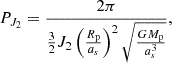
Stable orbits for potential satellites around WASP-49Ab are expected to exist within a narrow region bounded by the Roche limit (rR) and the Hill radius (rH). The Roche limit represents the minimum distance at which a satellite can avoid tidal disruption by the planet. For a satellite with mass Ms and radius Rs, rR is given by
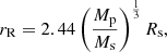 (1)
(1)
where Mp is the planet’s mass. Within this limit the tidal forces would exceed the moon’s self-gravity, leading to disintegration.
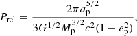
The outer stability boundary is defined by the secondary Hill radius, 4.8 rH for prograde orbits (Domingos et al. 2006). The Hill radius (rH) defines the region where the planet’s gravitational influence dominates over that of the star, calculated as
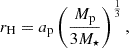 (2)
(2)
where ap is the semi-major axis of the planet’s orbit around the star and M⋆ is the mass of the host star. For WASP-49Ab, this region extends up to approximately 3.4 Rp, beyond which the star’s gravity would likely eject the satellite by mean of evection and eviction resonances that affect the satellite’s eccentricity and inclination, respectively (Vaillant & Correia 2022).
Thus, the stable orbital region for potential satellites around WASP-49Ab is constrained between the Roche limit and the secondary Hill radius, forming a delicate balance where satellites could survive the strong tidal and gravitational forces from both the planet and the host star.
2.2. Perturbative forces and orbital evolution of satellites
Satellite stability in this narrow region and extreme environment is influenced by various perturbative forces, which affect orbital parameters over different timescales. In the following, we detail these effects (see also Appendix A).
Stellar and planetary tides. Tidal interactions from both the host star and the planet play a crucial role in shaping the orbital evolution of satellites and planets, particularly in close-in systems like WASP-49Ab (see e.g. Makarov & Efroimsky 2023, and references therein). Stellar tides induce bulges on the planet, leading to energy dissipation and a gradual evolution of the satellite’s orbit. The rates of change in the semi-major axis and orbital period due to these tidal forces are described in Eqs. (9) and (10) in Alvarado-Montes et al. (2017), based on the framework by Barnes & O’Brien (2002) and the classical tidal dissipation model of Goldreich & Soter (1966), for a system where the planet’s physical characteristics evolve over time.
Here we assume the moon has survived any detachment processes and has reached its asymptotic semi-major axis, astop, defined by Sucerquia et al. (2020) as the orbital distance beyond which tidal forces no longer affect the moon’s orbit. This model assumes a slowly evolving planetary interior, but the planet’s close proximity to its star could result in elevated temperatures, affecting its size and internal structure, which should affect the long-term stability of the satellite’s orbit.
Perturbations from an outer body. In non-coplanar three-body systems, secular perturbations, including von Zeipel-Kozai-Lidov (ZLK) oscillations and periapsis precession (von Zeipel 1910; Lidov 1962; Kozai 1962; Hamers et al. 2018), can significantly impact long-term stability. In the WASP-49 system, these perturbations act through interactions between the planet and WASP-49B, affecting the planet’s orbital pa3rameters over tens of thousands of years, and through interactions between the satellite, the planet, and the primary star, influencing the satellite’s orbit on shorter timescales (weeks to months). For WASP-49Ab, ZLK effects driven by the binary companion are negligible due to the large separation and weak planetary perturbations. Similarly, periapsis precession of the planet due to the stellar companion should occur at a slow rate (∼10−7 rad/yr) and has a negligible impact on satellite stability. However, stellar-induced ZLK effects on satellites with inclinations (i > 39°) could cause destabilising eccentricity and inclination oscillations, making them highly prone to instability within 1.2–1.8 Rp. Consequently, such high-inclination satellites are excluded from this study.
Planetary oblateness. Due to its close proximity to the host star, WASP-49Ab is presumed to be tidally locked, meaning that its rotational period is synchronised with its orbital period. This tidal locking promotes a stable orientation, leading to an enhanced equatorial bulge or oblateness, which introduces additional gravitational perturbations affecting the orbits of any satellites. The gravitational influence of planetary oblateness is quantified by the gravitational harmonic coefficients J. The dominant term, J2 (quadrupole moment), represents the primary deviation from a perfect sphere and significantly affects satellite dynamics by inducing precession of the satellite’s argument of periastron, ω, with an effect that weakens with distance. In systems with an oblate host planet, the increased nodal precession rate induced by J2 stabilises the satellite’s orbit by preventing secular resonances with the host, which could otherwise destabilise the satellite’s inclination and eccentricity. This effect, as demonstrated by Hong et al. (2015), mitigates the destabilising influence of the moon’s inclination and enhances overall orbital stability relative to configurations with a spherical host planet. In this analysis we include only the J2 term to account for the primary stabilising effect of planetary oblateness on the satellite’s orbit. The rate of change in the planet’s periastron, ωJ, due to J2 is expressed as
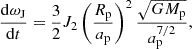 (3)
(3)
where Rp denotes the planet’s radius, ap its semi-major axis, Mp its mass, and G the gravitational constant. This precession effect can lead to significant changes in the orbital orientation of close-in satellites over time, contributing to the long-term stabilisation of their orbits by damping inclination and eccentricity variations.
To calculate the shape coefficient J2, it was assumed that its rotation period equals its orbital period (Prot = Porb). With this assumption, the angular velocity Ω was calculated as  . Then we obtained J2 using the equation
 (4)
(4)
where Mp and Rp are the planet’s mass and radius, respectively. With an estimated J2 ≈ 0.0063, which indicates greater oblateness than Earth but less than Jupiter, this coefficient suggests a substantial equatorial bulge driven by centrifugal forces, resulting in a pronounced deviation from sphericity. Such high oblateness could notably impact the planet’s gravitational field, its dynamical evolution, and the orbital dynamics of nearby satellites.
Relativistic effects. Due to the close proximity of WASP-49Ab to its star, relativistic effects introduce an additional rate of precession, ωGR, described by
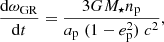 (5)
(5)
where M⋆ is the stellar mass, ep denotes the planet’s orbital eccentricity, c is the speed of light, and np = 2π/Pp is the planet’s mean orbital frequency, with Pp representing the orbital period. This relativistic correction leads to a continuous, gradual shift in the orientation of the planet’s elliptical orbit around its star. Although the effect is subtle per orbit, it accumulates significantly over many orbital cycles, resulting in a measurable advance of the pericentre position (see e.g. Jordán & Bakos 2008).
3. Methodology
3.1. Dynamical evolution
We investigated the stability of hypothetical satellites around WASP-49Ab using the REBOUND N-body code (Rein & Liu 2012), with additional physics from the REBOUNDx package (Tamayo et al. 2020). The system comprises a star, a planet, and an array of non-mutually interacting moons, configured to explore a wide range of orbital and physical parameter spaces. These satellites experience perturbations as outlined in Sect. 2. Specifically, we calculated the Mean Exponential Growth Factor of Nearby Orbits (MEGNO) parameter to get an insight into the general dynamical features system (Cincotta & Simó 2000).
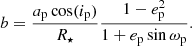
Additionally, we assessed the likelihood of satellite retention under various dynamical conditions, incorporating first-order relativistic corrections and planetary oblateness up to J2. This analysis led to the development of a metric termed selenity that quantifies a satellite’s ability to remain bound to its planet despite external perturbations. The metric is derived from simulations across the (as, es) or (as, ms) parameter spaces, evaluated over varying inclinations. For each point, the ratio of stable outcomes (bound satellites) to total cases is computed, yielding a normalised value between 0 and 1. This ensures that the satellite’s semi-major axis remains within the primary Hill radius, that its eccentricity stays between 0 and 1, and that it avoids collisions with the planet. Collectively, these criteria establish whether the satellite maintains a stable bounded orbit within the system’s dynamical constraints.
To compute the Roche radius (Eq. (1)) for the satellite radius, we adopted a mass–radius scaling relation applicable to rocky moons, with the form R ∝ M1/3.5, based on Io’s characteristics, but without adjustments for core mass fraction variations (Sotin et al. 2007). This approach provides a representative scale for rocky bodies similar to Io, but without specific composition dependence. We set the eccentricity of WASP-49Ab to an average value of 0.03, given the range variation between 0.0 and 0.05, based on the posterior probability distribution obtained from the MCMC analysis done by Wyttenbach et al. (2017). Given the short orbital period of the planet and the anticipated orbital periods of potential moons on the scale of hours, we selected the Hamiltonian WHFast integrator for the system’s evolution as close encounters are not a primary focus. A timestep of 10−5 yr was used, mapping the planet’s orbit with approximately 800 points and the moon’s orbit with about 70 points per cycle. Each simulation was conducted over 1000 planetary periods, encompassing approximately 105 orbits of a hypothetical moon with an orbital period of roughly ten hours. This set-up allows for a comprehensive exploration of satellite dynamics across a wide range of configurations (see Appendix A for details on the timescales).
3.2. Detectability of exomoons around WASP-49Ab
A planet with a massive satellite orbits the centre of mass of the planet-satellite system, causing TTVs and TDVs due to changes in the planet’s position and velocity relative to this centre of mass during transits. TTV signals are most pronounced for circular coplanar orbits and for edge-on systems. The root mean square (rms) TTV amplitude, δTTV, and TDV amplitude, δTDV, are given by (Kipping 2009b)
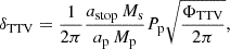 (6)
(6)
 (7)
(7)
where ΦTTV → π for aligned circular orbits. Moreover,  is the averaged transit duration given by
![Mathematical equation: $$ \begin{aligned} \bar{\tau } = \frac{P_{\rm p}}{\pi } \arcsin {\left[\sqrt{\frac{(R_* + R_{\rm p})^2 - (b R_*)^2}{a_{\rm p}^2 - b^2 R_*^2 }}\right]}, \end{aligned} $$](/articles/aa/full_html/2025/02/aa52968-24/aa52968-24-eq10.gif) (8)
(8)
where Ps is the moon’s orbital period and R* is the stellar radius. Equations (6) and (7) do not depend on the moon’s apparent size, making them independent of secondary effects such as an atmosphere or extended material around the moon. However, a massive moon can produce significant TTV and TDV signals, with amplitudes directly proportional to the moon’s mass. Additionally, simultaneous transits of the moon can alter the perceived depth of the transit, either within a single transit or across multiple transits, depending on the orbital periods of the moon and the planet.
4. Results and analysis
4.1. Exomoon dynamics
In Fig. 1 we highlight the regions where moons are most likely to remain stable. The colour scale in each panel represents the selenity metric: a selenity value of 1 indicates strong gravitational binding to the planet and a value of 0 indicates that the satellite is unbound. Intermediate values suggest partial instability, primarily influenced by the satellite’s initial inclination.
 |
Fig. 1. Stability maps illustrating survival and ejection probabilities for exomoons orbiting a close-in giant planet, factoring in the planet’s J2 quadrupole moment and relativistic corrections over 1000 Pp. The colour scale indicates the selenity, which shows the moon’s likelihood of remaining bound to the planet under external perturbations. The left panel shows stability in the as − es plane, with the Roche limit and Hill radius as key markers. The right panel displays stability in the as − Ms plane, reflecting stability variations based on satellite mass and planet distance. |
The left panel of Fig. 1 shows the stability map in the as − es plane, where as is the semi-major axis in units of planetary radii (Rp) and es is the orbital eccentricity. Each point in the simulation, representing a specific combination of semi-major axis and eccentricity, was evaluated across five different inclinations ranging from 0° to 39°, ensuring that the effects of potentially destabilising resonances, such as ZLK resonances, were adequately accounted for and mitigated. The results were then combined (stacked) and normalised to create a unified stability map. Two key dynamical boundaries are highlighted: the red dashed line marking the Roche limit and the purple dashed line denoting the Hill radius. The light green regions indicate high orbital stability, where satellites are likely to remain bound, while the blue regions represent areas with a higher probability of ejection. In this configuration, the calculated survival rate for satellites is 24.9%. The right panel of Fig. 1 displays the stability map in the as − ms plane for circular orbits, where ms is the satellite’s mass in units of Io’s mass (mIo). The light orange regions denote configurations with greater orbital stability, where satellites show a survival rate of 47.2%, while the dark brown to black areas highlight regions of increased ejection probability. The labelled lines mark the Roche radii, varying with satellite mass, representing the minimum safe distances from tidal disruption.
These stability maps, which align with and complement the MEGNO stability maps shown in Fig. B.1, provide valuable insights into the survival constraints for satellites in the WASP-49Ab system, particularly highlighting resilient orbital configurations. Notably, the Rebound implementation of the MEGNO indicator focuses on Newtonian dynamics, whereas selenity accounts for more complex interactions and environmental factors.
In summary, potential satellites in this system must reside very close to their planet, with low eccentricities (up to 0.2) and low inclinations. Furthermore, stability improves for satellites with masses similar to or greater than Io’s. Masses below this threshold render the system unstable, while higher masses contribute to stability, but cannot exceed five times Io’s mass to satisfy the Ms/Mp ≤ 10−4 ratio found by Canup & Ward (2006).
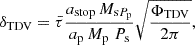
4.2. Transit features and relativistic effects
The restricted range of values for the planet’s mass and semi-major axis imposes significant constraints on its detectability via indirect dynamical methods. Applying Eqs. (6) and (7) to the most optimistic estimates for ms and as from Sect. 4.1, the predicted transit timing and duration variations remain under a fraction of a minute. However, due to the extreme proximity of WASP-49Ab to its host star, relativistic precession and planetary deformation introduce a cumulative shift in the orientation of the orbital plane, which can affect the observed impact parameter and transit duration (Jordán & Bakos 2008), potentially mimicking satellite-induced variations and complicating interpretation.
The rate of periastron precession, influenced by both general relativistic effects and the planet’s complex gravitational potential, affects ωGR and ωp over time, as given by Eqs. (5) and (3). This precession causes a gradual rotation of the orbital plane, impacting The impact parameter b is defined as the projected distance, in units of the stellar radius, between the centre of the planet and the centre of the star at mid-transit. Notably, b is particularly sensitive to this precession:
 (9)
(9)
Here R⋆ denotes the stellar radius and i is the orbital inclination. As the argument of periastron ωp progresses, slight variations in b occur, modulating the transit geometry and consequently affecting the transit duration. Last, the transit duration  , which depends on both the impact parameter and the orbital velocity of the planet at mid-transit, can be estimated by Eq. (8).
Over a timescale of 100 years (∼13 000 orbits), we calculate a cumulative transit duration change, δτ, of approximately 1.3 minutes for an Io analogue at 1.3 Rp, resulting from relativistic and oblateness-induced precession. Figure 2 illustrates, in the left panel, the short-term evolution of ϖ, b, and  over time, while the right panel highlights the gradual drift in transit duration over a century. On shorter timescales (left panel), small shifts in frequency and amplitude become noticeable after a single planetary period across different models: Newtonian (solid lines) and relativistic (dashed lines), each evaluated with (wm) and without (nm) a massive moon. In the nm model, amplitudes are approximately an order of magnitude lower than in the wm model. Although these rms amplitude variations are small (δb ∼ 10−3 and
  ), they may still influence noise levels in detection efforts. Over longer timescales, however, the most significant effect appears in the full model, showing a cumulative shift in the argument of pericentre of approximately 13° per century.
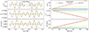 |
Fig. 2. Evolution of the argument of pericentre (ϖp), the impact parameter (b), and the transit duration ( |

5. Discussion and conclusions
We investigated the evolution of hypothetical satellites around the close-in warm Saturn WASP-49Ab, considering its complex dynamical environment, including planetary deformation and general relativistic effects, within a numerical framework. Our focus was on satellites inside the narrow region between the Roche limit and the secondary Hill radius, constrained to moderate eccentricities and inclinations. Through a series of simulations assessing the MEGNO indicator and the selenity metric (see Sect. 3), we found that stability is favoured for moons with masses similar to Io.
The MEGNO and selenity maps revealed a chaotic region around as ≈ 1.4 Rp, initially suspected to result from mean-motion resonances. However, a detailed analysis of semi-major axes from 1.3 to 1.5 Rp found no significant mean-motion resonances up to the fifth order, suggesting that the chaos is not driven by such resonances. The selenity metric further constrained the semi-major axis and eccentricity ranges for which moons remain bound to the planet, keeping the eccentricities of surviving moons below 0.22. Notably, even with significant inclinations, the moons displayed considerable stability. This is attributed to the oblate shape of the host planet, which enhances the nodal precession rate, thereby mitigating destabilising secular resonances as was described by Hong et al. (2015). Moreover, in simulations where ep was initialised to zero, the chaotic behaviour was eliminated, indicating that secular precession effects induced by the planet’s eccentricity are the primary cause, likely arising from a ν-type secular resonance.
From a detectability perspective, we found that the δTTV and δTDV signals are below tenths of a minute, making them undetectable with current instrumentation. However, relativistic effects and the planet’s rotational deformation significantly alter the rate of change in the planet’s argument of pericentre, ϖp. Over long timescales, this causes a gradual shift in the orbital orientation and modifies the transit duration. This effect is more pronounced for eccentric orbits, but for WASP-49Ab, we estimate a cumulative impact on transit duration of approximately 1.3 minutes per century. On shorter timescales, by contrast, we observed an oscillatory pattern in the planet’s impact parameter, affecting its third decimal place. Such variations may affect parameter estimates across studies over different epochs.
In summary, even in extreme environments like that of WASP-49Ab, we find that exomoons can remain dynamically stable. We also demonstrated that accurate exomoon detection requires that various sources of gravitational perturbations be accounted for, including stellar multiplicity, higher-order gravitational effects, and interactions with other planets or sibling satellites. This work provides a general framework to motivate, guide, and support the upcoming search for exomoons.
Such as those explored by Carles Simó; see e.g. https://bgsmath.cat/people/?person=carles-simo
Acknowledgments
This project was supported by the European Research Council (ERC) under the European Union Horizon Europe research and innovation program (grant agreement No. 101042275, project Stellar-MADE). We also thank MSP and the Stellar-MADE team for their kind support.
References
- Alvarado-Montes, J. A., Zuluaga, J. I., & Sucerquia, M. 2017, MNRAS, 471, 3019 [CrossRef] [Google Scholar]
- Barnes, J. W., & Fortney, J. J. 2004, ApJ, 616, 1193 [NASA ADS] [CrossRef] [Google Scholar]
- Barnes, J. W., & O’Brien, D. P. 2002, ApJ, 575, 1087 [NASA ADS] [CrossRef] [Google Scholar]
- Canup, R. M., & Ward, W. R. 2006, Nature, 441, 834 [NASA ADS] [CrossRef] [Google Scholar]
- Cincotta, P. M., & Simó, C. 2000, A&AS, 147, 205 [NASA ADS] [CrossRef] [EDP Sciences] [Google Scholar]
- Domingos, R. C., Winter, O. C., & Yokoyama, T. 2006, MNRAS, 373, 1227 [NASA ADS] [CrossRef] [Google Scholar]
- Goldreich, P., & Soter, S. 1966, Icarus, 5, 375 [Google Scholar]
- Gordon, B. R., Buschermöhle, H., Tubthong, W., et al. 2024, ApJ, submitted [arXiv:2412.02847] [Google Scholar]
- Hamers, A. S., Cai, M. X., Roa, J., & Leigh, N. 2018, MNRAS, 480, 3800 [NASA ADS] [CrossRef] [Google Scholar]
- Heller, R. 2018, A&A, 610, A39 [NASA ADS] [CrossRef] [EDP Sciences] [Google Scholar]
- Hong, Y.-C., Tiscareno, M. S., Nicholson, P. D., & Lunine, J. I. 2015, MNRAS, 449, 828 [NASA ADS] [CrossRef] [Google Scholar]
- Jordán, A., & Bakos, G. Á. 2008, ApJ, 685, 543 [CrossRef] [Google Scholar]
- Kipping, D., Bryson, S., Burke, C., et al. 2022, Bulletin of the American Astronomical Society, 54, 504.04 [NASA ADS] [Google Scholar]
- Kipping, D. M. 2009a, MNRAS, 392, 181 [NASA ADS] [CrossRef] [Google Scholar]
- Kipping, D. M. 2009b, MNRAS, 396, 1797 [NASA ADS] [CrossRef] [Google Scholar]
- Kozai, Y. 1962, AJ, 67, 591 [Google Scholar]
- Kreidberg, L., Luger, R., & Bedell, M. 2019, ApJ, 877, L15 [NASA ADS] [CrossRef] [Google Scholar]
- Lendl, M., Anderson, D. R., Collier-Cameron, A., et al. 2012, A&A, 544, A72 [NASA ADS] [CrossRef] [EDP Sciences] [Google Scholar]
- Lidov, M. L. 1962, Planet. Space Sci., 9, 719 [Google Scholar]
- Makarov, V. V., & Efroimsky, M. 2023, A&A, 672, A78 [NASA ADS] [CrossRef] [EDP Sciences] [Google Scholar]
- Martínez-Rodríguez, H., Caballero, J. A., Cifuentes, C., Piro, A. L., & Barnes, R. 2019, ApJ, 887, 261 [Google Scholar]
- Oza, A. V., Seidel, J. V., Hoeijmakers, H. J., et al. 2024, ApJ, 973, L53 [NASA ADS] [CrossRef] [Google Scholar]
- Quarles, B., Eggl, S., Rosario-Franco, M., & Li, G. 2021, AJ, 162, 58 [NASA ADS] [CrossRef] [Google Scholar]
- Rein, H., & Liu, S. F. 2012, A&A, 537, A128 [NASA ADS] [CrossRef] [EDP Sciences] [Google Scholar]
- Rodenbeck, K., Heller, R., & Gizon, L. 2020, A&A, 638, A43 [NASA ADS] [CrossRef] [EDP Sciences] [Google Scholar]
- Sotin, C., Grasset, O., & Mocquet, A. 2007, Icarus, 191, 337 [Google Scholar]
- Sucerquia, M., Alvarado-Montes, J. A., Bayo, A., et al. 2022, MNRAS, 512, 1032 [NASA ADS] [CrossRef] [Google Scholar]
- Sucerquia, M., Alvarado-Montes, J. A., Zuluaga, J. I., Cuello, N., & Giuppone, C. 2019, MNRAS, 489, 2313 [NASA ADS] [CrossRef] [Google Scholar]
- Sucerquia, M., Ramírez, V., Alvarado-Montes, J. A., & Zuluaga, J. I. 2020, MNRAS, 492, 3499 [NASA ADS] [CrossRef] [Google Scholar]
- Tamayo, D., Rein, H., Shi, P., & Hernandez, D. M. 2020, MNRAS, 491, 2885 [NASA ADS] [CrossRef] [Google Scholar]
- Teachey, A., Kipping, D. M., & Science, 2018, Advances, 4, eaav1784 [NASA ADS] [Google Scholar]
- Vaillant, T., & Correia, A. C. M. 2022, A&A, 657, A103 [NASA ADS] [CrossRef] [EDP Sciences] [Google Scholar]
- von Zeipel, H. 1910, Astronomische Nachrichten, 183, 345 [Google Scholar]
- Wyttenbach, A., Lovis, C., Ehrenreich, D., et al. 2017, A&A, 602, A36 [NASA ADS] [CrossRef] [EDP Sciences] [Google Scholar]
Appendix A: Dynamical timescales
The dynamical timescales of a hypothetical satellite in the WASP-49Ab system are governed by gravitational interactions, relativistic effects, and the planet’s oblateness. These processes collectively determine the evolution of the satellite’s orbit. Below, we summarise the origin of the timescales in Table A.1.
Dynamical effects and their associated timescales in the WASP-49Ab system.
The timestep in our simulations is determined by the shortest dynamical timescale in the system. As shown in Table A.1, the orbital period of the moon is the fastest process, ranging from approximately 7 × 10⁻⁴ to 1.3 × 10⁻³ yr (6–11 h). To ensure numerical stability and accuracy, we adopt a timestep of 10−5 yr for the maps presented in Figs. 1, B.1, and B.2. This is over two orders of magnitude smaller than the shortest relevant timescale, enabling precise resolution of rapid precession and satellite orbital motion without incurring excessive computational cost.
Both the satellite’s orbital period and that of the binary star are governed by Kepler’s third law. For the binary system, this may be expressed as
where a2 is the semi-major axis of the secondary’s orbit, M1 is the mass of the primary, M2 is the mass of the secondary, and G is the gravitational constant. The range of orbital periods presented in Table A.1 reflects distances spanning from the Roche limit to 1.5 planetary radii.
The Zeipel-Kozai-Lidov (ZLK) effect in the binary system causes oscillations in the planet’s inclination and eccentricity due to perturbations from the distant stellar companion. The characteristic timescale for this effect is
 (A.1)
(A.1)
where Pbin is the orbital period of the binary system, Pp is the orbital period of the planet, M⋆ is the host star’s mass, and Mbin is the mass of the stellar companion.
For the satellite, the Kozai–Lidov effect induces oscillations in its inclination and eccentricity due to the gravitational influence of the host star. The timescale for this process is given by
 (A.2)
(A.2)
where Ps is the satellite’s orbital period.
The oblateness of the planet, represented by J2, leads to precession of the satellite’s orbital plane. The timescale for this effect is
 (A.3)
(A.3)
where Rp is the planet’s radius and as is the semi-major axis of the satellite’s orbit. Here we assumed that the satellite’s orbital eccentricity es = 0 and inclination is = 0.
General relativistic effects cause the precession of the planet’s periapsis. The associated timescale is
 (A.4)
(A.4)
where ap and ep are the planet’s semi-major axis and eccentricity, and c is the speed of light. In addition, relativistic effects can influence the satellite indirectly, through the planet’s periapsis precession, as well as directly via the gravitational gradient associated with its own orbital motion. These influences have seldom been explored, largely because the existence of satellites in such close proximity to their host stars was not anticipated. Employing secular theory to investigate these phenomena could yield valuable insights into their cumulative impact over long timescales, particularly given the broad diversity of temporal scales involved.
The ranges of timescales presented in Table A.1 reflect the satellite’s orbital distance spanning from the Roche limit to 1.5 planetary radii. These variations illustrate the sensitivity of the dynamical timescales to the satellite’s orbital configuration and the underlying physical processes.
Appendix B: Stability maps
The MEGNO stability maps shown in Fig. B.1 illustrate the dynamical behaviour of hypothetical moons around WASP-49Ab, focusing on the coplanar configuration. When the satellite’s eccentricity is set to zero (upper panel in Fig. B.1), no instability gap is observed, emphasising the stabilising role of a circular orbit. However, when the planet’s eccentricity is non-zero (lower panel in Fig. B.1), a distinct instability gap appears near 1.4 Rp, which shifts to larger semi-major axes as the satellite’s inclination increases in other maps (not shown). This gap is not associated with mean-motion resonances but rather arises from the planet’s eccentricity, which induces secular perturbations that destabilise the satellite’s orbit in specific regions.
The simulations were conducted using a timestep of 10−5 yr, ensuring precise resolution of the satellite’s orbital dynamics. Each simulation covered 1000 planetary orbits, equivalent to nearly 105 satellite periods, providing a comprehensive assessment of the system’s stability over long timescales.
The MEGNO indicator used here relies on a Newtonian point-mass model, which excludes effects such as planetary Jn zonal deformation and relativistic corrections. These limitations stem from its implementation in codes like REBOUND, rather than the MEGNO framework itself. In principle, MEGNO can extend beyond classical N-body dynamics, provided the equations of motion incorporate conservative forces. Examples include the Schwarzschild relativistic correction, the conservative tidal distortion potential, and the J2 zonal deformation effect.
Moreover, MEGNO is compatible with non-autonomous systems, where time explicitly appears as a variable in the equations of motion. This has been demonstrated in studies of systems with effective 1 degree of freedom, derived from three coordinates and two constraints 1. For the dynamical maps presented, Newtonian forces dominate the short-term dynamics, justifying the first-order approximation. Comparisons with the ‘selenity’ factor further validate this approach as a robust representation of the core dynamics, despite minor unmodelled perturbations. However, as shown in the MEGNO and selenity maps in Figs. 1, B.1, and B.2, the instability near 1.4 Rp persists even when these additional effects are included, indicating that it is a robust dynamical feature of the system. This instability does not appear when the planet’s eccentricity is set to zero (ep = 0), suggesting that it is primarily driven by gravitational and secular perturbations related to the planet’s non-zero eccentricity (ep ≠ 0). These perturbations cause oscillations in the satellite’s orbital elements, particularly eccentricity, potentially leading to destabilising scenarios like perigee near the Roche limit or apogee beyond the secondary Hill radius. The recurrence of this instability in both MEGNO and selenity maps suggests a secular resonance, possibly ν-type, though confirmation requires detailed secular theory analysis.
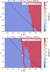 |
Fig. B.1. MEGNO stability maps showing regular orbits over 1000 Pp, with key limits marked by the Roche limit (in red) and Hill radius (in black). The top panel assumes a planetary eccentricity of ep = 0, while the bottom panel assumes ep = 0.03. |
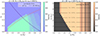 |
Fig. B.2. Stability maps showing exomoon survival and ejection probabilities around a close-in giant planet, considering J2 and relativistic effects over 1000 Pp for a planet with a circular orbit (ep = 0). The colour scale represents ‘Selenity’, indicating the likelihood of moons remaining bound. Left: Stability in the as − es plane, with the Roche limit and Hill radius marked. Right: Stability in the as − Ms plane, highlighting variations with satellite mass and planet distance. |
To further investigate the role of satellite mass on stability, we conducted additional simulations for Ms = 0.1 MIo and Ms = 0.01 MIo. The survival rates decreased markedly, from 25% for Ms = MIo to 17% and 16%, respectively. This finding confirms that satellite mass plays a significant role in the system’s dynamics, as smaller masses reduce the satellite’s gravitational influence and its ability to resist destabilising perturbations. These effects are particularly apparent near 1.4 Rp, where the interplay between the planet’s eccentricity-driven secular perturbations and the satellite’s reduced stabilising influence leads to enhanced instability.
This result strengthens the trends observed in Fig. 1, indicating that satellites with masses below MIo are increasingly prone to destabilisation. Such findings suggest a practical lower limit on the masses of stable satellites in systems like WASP-49Ab, highlighting the crucial role of satellite mass in long-term dynamical stability.
All Tables
All Figures
|
Fig. 1. Stability maps illustrating survival and ejection probabilities for exomoons orbiting a close-in giant planet, factoring in the planet’s J2 quadrupole moment and relativistic corrections over 1000 Pp. The colour scale indicates the selenity, which shows the moon’s likelihood of remaining bound to the planet under external perturbations. The left panel shows stability in the as − es plane, with the Roche limit and Hill radius as key markers. The right panel displays stability in the as − Ms plane, reflecting stability variations based on satellite mass and planet distance. |
| In the text | |
|
Fig. 2. Evolution of the argument of pericentre (ϖp), the impact parameter (b), and the transit duration ( |
| In the text | |
|
Fig. B.1. MEGNO stability maps showing regular orbits over 1000 Pp, with key limits marked by the Roche limit (in red) and Hill radius (in black). The top panel assumes a planetary eccentricity of ep = 0, while the bottom panel assumes ep = 0.03. |
| In the text | |
|
Fig. B.2. Stability maps showing exomoon survival and ejection probabilities around a close-in giant planet, considering J2 and relativistic effects over 1000 Pp for a planet with a circular orbit (ep = 0). The colour scale represents ‘Selenity’, indicating the likelihood of moons remaining bound. Left: Stability in the as − es plane, with the Roche limit and Hill radius marked. Right: Stability in the as − Ms plane, highlighting variations with satellite mass and planet distance. |
| In the text | |
Current usage metrics show cumulative count of Article Views (full-text article views including HTML views, PDF and ePub downloads, according to the available data) and Abstracts Views on Vision4Press platform.
Data correspond to usage on the plateform after 2015. The current usage metrics is available 48-96 hours after online publication and is updated daily on week days.
Initial download of the metrics may take a while.