| Issue |
A&A
Volume 708, April 2026
|
|
|---|---|---|
| Article Number | A342 | |
| Number of page(s) | 8 | |
| Section | The Sun and the Heliosphere | |
| DOI | https://doi.org/10.1051/0004-6361/202557966 | |
| Published online | 28 April 2026 | |
Inferring physical parameters of solar filaments from simultaneous longitudinal and transverse oscillations
1
Aryabhatta Research Institute of Observational Sciences, 263001 Nainital, India
2
Department of Applied Physics, Mahatma Jyotiba Phule Rohilkhand University, Bareilly, 243006 Uttar Pradesh, India
3
Instituto de Astrofísica de Canarias, E-38205 La Laguna, Tenerife, Spain
4
Departamento de Astrofísica, Universidad de La Laguna, E-38206 La Laguna, Tenerife, Spain
★ Corresponding author: This email address is being protected from spambots. You need JavaScript enabled to view it.
Received:
4
November
2025
Accepted:
26
December
2025
Abstract
Context. Different modes of oscillations are frequently observed in solar prominences, and prominence seismology helps estimate important physical parameters such as the magnetic field strength. Although the simultaneous detection of longitudinal and transverse oscillations in the same filament is not common, such rare observations provide a unique opportunity to constrain the physical parameters of interest.
Aims. In this study, we aim to estimate the physical parameters of prominences undergoing simultaneous longitudinal and transverse oscillations.
Methods. We applied Bayesian seismology techniques to observations of longitudinal and transverse filament oscillations to infer the magnetic field strength, the length, and the number of twists in the flux tube holding the prominence plasma. We first used the observations of longitudinal oscillations and the pendulum model to infer the posterior probability density for the magnetic field strength. The obtained marginal posterior of the magnetic field, combined with the observations of the transverse oscillations, was then used to estimate the probable values of the length of the magnetic flux tube that supports the filament material using Bayesian inference. This estimated length was used to compute the number of twists in the flux tube.
Results. For the prominences under study, we find that the length of the flux tubes supporting the quiescent prominences can be very large (from 100 to 1000 Mm), and the number of twists in the flux tube is not more than three.
Conclusions. Our results demonstrate that Bayesian analysis offers valuable methods for parameter inference in prominence seismology.
Key words: Sun: filaments / prominences / Sun: oscillations
© The Authors 2026
 Open Access article, published by EDP Sciences, under the terms of the Creative Commons Attribution License (https://creativecommons.org/licenses/by/4.0), which permits unrestricted use, distribution, and reproduction in any medium, provided the original work is properly cited.
This article is published in open access under the Subscribe to Open model. This email address is being protected from spambots. You need JavaScript enabled to view it. to support open access publication.
1. Introduction
Understanding the internal structure, dynamics, and energetics of solar prominences is challenging. However, the presence of oscillations in the filaments, detected using Hα spectrograms (Dyson 1930) and extreme ultraviolet (EUV) observations (Li & Zhang 2012; Liu et al. 2013) is a useful source of information. Depending on velocity amplitudes, prominence oscillations are classified into two categories (Oliver & Ballester 2002; Arregui et al. 2018). The first consists of large amplitude oscillations in which the entire prominence – or most of it – experiences oscillations with velocity amplitudes greater than 10 km s−1 (Okamoto et al. 2004; Tripathi et al. 2009; Kucera et al. 2022; Joshi et al. 2023). The second consists of small amplitude oscillations that affect localised regions of the prominence and have velocity amplitudes of a few (2-3) kilometres per second (Yi & Engvold 1991; Yi et al. 1991; Engvold et al. 2000; Oliver & Murdin 2001; Oliver & Ballester 2002; Ning et al. 2009; Soler et al. 2011).
Prominences support both longitudinal and transverse oscillations. If the periodic motion of the plasma is along the magnetic field, the oscillations are called longitudinal oscillations. First observations of such longitudinal oscillations were reported using Hα observations performed at the Big Bear Solar Observatory (Jing et al. 2003, 2006). Longitudinal oscillations are triggered when a small energetic event, such as a sub-flare, flare, or small jet, occurs near the footpoint of the filament (Jing et al. 2003, 2006; Luna et al. 2014; Zhang et al. 2017; Dai et al. 2021). Not only do nearby flares trigger, but they can sometimes also enhance the longitudinal oscillations (Zhang et al. 2020). Additionally, the merging of two filaments can also trigger large amplitude longitudinal oscillations (Luna et al. 2017). Initially, magnetic tension (Jing et al. 2003, 2006) and/or magnetic pressure gradients (Vršnak et al. 2007) were considered to be the restoring force of such oscillations. Later, Luna & Karpen (2012), Luna et al. (2012, 2022) provided a theoretical model known as the ’pendulum model’ to explain these longitudinal oscillations.
Apart from these longitudinal oscillations, motions perpendicular to the magnetic field direction are also observed. Depending on the direction of oscillations, they can be either vertical or horizontal motions of the filaments and are collectively known as transverse oscillations of the filaments (Ramsey & Smith 1966; Hyder 1966; Kleczek & Kuperus 1969; Lin et al. 2009; Hershaw et al. 2011; Liu et al. 2012; Gosain & Foullon 2012; Pant et al. 2015; Devi et al. 2022; Dai et al. 2023; Zhang et al. 2024).
A few studies have reported simultaneous longitudinal and transverse oscillations in the same prominence or prominence threads (Okamoto et al. 2007; Gilbert et al. 2008; Pant et al. 2016; Tan et al. 2023). Pant et al. (2016) reported both longitudinal and transverse oscillations in an active region filament triggered after being hit by a shock wave. Zhang et al. (2017) reported longitudinal and transverse oscillations in the same quiescent prominence triggered by a jet. Mazumder et al. (2020), Dai et al. (2021) also reported simultaneous longitudinal and transverse oscillations in quiescent filaments. Recently, both wave modes have been observed in a filament excited by EUV waves (Pan et al. 2025). Additionally, 3D motions of filaments have also been probed through horizontal and vertical transverse oscillations (Isobe & Tripathi 2006; Dai et al. 2023).
Combining these observations with magnetohydrodynamic (MHD) wave theory can help estimate such physical parameters as magnetic field strength using seismological tools (Arregui et al. 2018). Prominence seismology was first suggested by Tandberg-Hanssen (1995) after the successful application of seismology in coronal loops (Uchida 1970; Roberts et al. 1984). Recently, Pant et al. (2016), Mazumder et al. (2020), Dai et al. (2021), Tan et al. (2023), Pan et al. (2025) have employed the so-called pendulum model to estimate the filament’s magnetic field and the curvature radius of the dip from observations of their longitudinal oscillations. Mazumder et al. (2020) further used this magnetic field to estimate the length of the magnetic field lines supporting the prominence material. These previous studies provide either point estimates and/or possible ranges of variation for the parameters of interest.
The use of Bayesian analysis in prominence seismology was first suggested by Arregui et al. (2014) and successfully applied to infer the magnetic field strength and transverse density length-scales in prominence threads by Montes-Solís & Arregui (2019). The main advantage of Bayesian methods for seismology inversions is their consistent treatment of incomplete and uncertain information, which makes impossible to obtain a unique solution (Arregui & Goossens 2019), requiring formulation as probability density distributions (Arregui 2018, 2022). These methods also correctly propagate the errors from observed data into uncertainty in the inferred parameters (Arregui & Asensio Ramos 2011).
This paper aims to investigate the application of Bayesian inference in analysing simultaneous longitudinal and transverse oscillations within the same prominence to estimate the associated physical parameters. To achieve this, we adopted a methodology similar to that of Mazumder et al. (2020). First, the magnetic field strength supporting the prominence thread was inferred and then used to determine the length of the flux tube, which was further used to estimate the twist number. However, in contrast to Mazumder et al. (2020), we explored the entire parameter space within the Bayesian framework. Thus, by considering the appropriate prior distributions, we obtained the posterior distribution of both length and the magnetic field strength holding the quiescent prominence flux tube. First, we present a brief description of Bayesian methodology in Section 2. Then, using the analysis of longitudinal oscillations in Mazumder et al. (2020), Pan et al. (2025), we discuss the probable values of magnetic fields obtained in Section 3.1. Combining these probable values of the magnetic field and analysis of the transverse oscillations, we determine the length of the field lines supporting the prominence material in Section 3.2. We also estimate the number of twists associated with these flux tubes in Section 3.3, after computing the radius of curvature of these field lines. Section 4 briefly summarises our work.
2. Methodology: Bayesian statistics
Given a model M with a parameter vector θ proposed to explain observed data d, Bayesian parameter inference relies on the use of the Bayes theorem:
 (1)
(1)
Here, the posterior probability distribution p(θ|d, M) is obtained from the combination of the likelihood function p(d|θ, M) and the prior probability density p(θ|M) and encompasses all the information that can be gathered from the assumed model and the observed data.
For multi-parameter models, θ = {θ1, ..., θi, ..., θN}, the probability of a particular parameter of interest can be obtained by marginalising the posterior probability distribution with respect to all the other parameters as follows:
 (2)
(2)
Thus, for parameter estimation using Bayesian inference, two pieces of information are required: the prior information and the likelihood function. In this study, all the parameters were considered to be independent; thus, the global prior is the product of the individual priors associated with each parameter. Three types of individual priors were considered here. Firstly, we considered that each parameter lies in a given plausible range, where all the values are equally probable, then a uniform prior of the form
 (3)
(3)
was adopted. Second, when more specific information about the parameter was available from observations, the gamma and Gaussian distributions were used as priors. The gamma distribution is considered positive and has no upper bound. A parametric form of the gamma distribution can be expressed as
 (4)
(4)
Here, α and β correspond to the shape and rate parameters. The distribution’s mean and coefficient of variance are given by α/β and α/β2, respectively. Alternatively, for a Gaussian prior, the mean (μθi) and the uncertainty (σθi) associated with the parameter can be used, and its distribution is of the form
![Mathematical equation: $$ \begin{aligned} \mathcal{G} (\theta _i; \mu _{\theta _i},\sigma _{\theta _i}) = \frac{1}{\sqrt{2\pi }\sigma _{\theta _i}} \exp {\left[\frac{-(\theta _i - \mu _{\theta _i})^2}{2\sigma _{\theta _i}^2}\right]}. \end{aligned} $$](/articles/aa/full_html/2026/04/aa57966-25/aa57966-25-eq5.gif) (5)
(5)
For the likelihood functions, Gaussian profiles were applied according to the normal error assumption, which can be expressed as
![Mathematical equation: $$ \begin{aligned} p(d|\theta , M) = \frac{1}{\sqrt{2\pi }\sigma _{d}} \exp {\left[\frac{-(d - d_{M}(\theta ))^2}{2\sigma _{d}^2}\right]}. \end{aligned} $$](/articles/aa/full_html/2026/04/aa57966-25/aa57966-25-eq6.gif) (6)
(6)
The exponential of the Equation (6) explicitly contains its dependence on the model M, which is assumed to be true. Notably, it does not convey the likelihood of various data occurrences but serves to quantify the disparity between model predictions and observed data relative to the uncertainty in the data. Consequently, it assigns varying likelihood levels to alternative parameter combinations.
Calculating posteriors and marginal probability distributions necessitates solving integrals within the parameter space. When dealing with a low-dimensional problem, for instance, in this work, direct numerical integration over a grid of points is viable, and the sampling of the posterior using Markov chain Monte Carlo (MCMC) methods serves as a practical alternative, applicable not only in low-dimensional but also in high-dimensional spaces. We followed the same approach as Montes-Solís & Arregui (2017, 2019), Baweja et al. (2024), and Zhong et al. (2025) and computed the required posteriors using both direct integration and MCMC sampling, ensuring that the results are consistent.
3. Analysis and results
In our analysis, we employed Bayesian methods to estimate the prominence physical parameters of interest, combining theoretical models with observations of simultaneous transversely and longitudinally oscillating quiescent prominences studied in Mazumder et al. (2020) and Pan et al. (2025). First, we used the period of longitudinal oscillations to constrain the magnetic field strength. We then used this information together with the transverse oscillation period to infer the length of the magnetic flux tube holding the prominence plasma. Finally, we estimated the twist number.
3.1. Inference of magnetic field strength from longitudinal oscillations
To estimate the magnetic field strength from the longitudinal oscillations, we adopted the pendulum model (Luna & Karpen 2012), in which the magnetic tension balances the projected gravity in the flux tube dip, such that
 (7)
(7)
Here, B is the magnetic field strength at the bottom of the dip, r is the radius of curvature of the dips containing the cool prominence plasma, m = 1.27mp (with mp as the proton mass), the mean particle mass (Aschwanden 2005), and ne the electron number density in the thread. The model was verified by multiwavelength analysis and numerical simulations of an active region prominence by Zhang et al. (2012). Recently, Luna et al. (2022) extended the model to consider non-uniform gravity and non-circular dips.
For the plasma to oscillate longitudinally in the prominences, the surface gravity (g0) of the Sun provides the main restoring force. Thus, the angular frequency (ω) of these longitudinal oscillations is given by
 (8)
(8)
Here, pl denotes the period of the longitudinal oscillations. Combining this equation with the pendulum model (Equation (7)) and substituting the mass m and g0 = 274 m s−1, a lower limit for the magnetic field strength in the prominence can be obtained as
![Mathematical equation: $$ \begin{aligned} \begin{aligned} B[\mathrm{G}] = 26\sqrt{\frac{n_{e}}{10^{11} \mathrm{{cm}}^{-3}}}\,p_l\,[\mathrm{hr}], \end{aligned} \end{aligned} $$](/articles/aa/full_html/2026/04/aa57966-25/aa57966-25-eq9.gif) (9)
(9)
provided the periodicity pl of the longitudinal oscillations is known. This equation can be further simplified to
 (10)
(10)
In what follows, we use pl and Pl to denote theoretical and observational longitudinal periods, respectively. Observationally, Luna et al. (2018) analysed longitudinal oscillations in 196 filaments and found the mean periodicity to be Pl = 58 ± 15 minutes. They assumed the typical values of electron number density (ne = 1010 − 1011 cm−3; Luna et al. 2014), in the pendulum model (Equation (7)) and obtained the average minimum value of the magnetic field (≈16 G) and radius of curvature of the magnetic dips in the filaments (≈89 Mm).
In our Bayesian analysis, we used Equation (10) as model Ml to obtain the probable range of minimum magnetic field strength from the observed periods of longitudinal oscillations Pl. This model depends on two parameters, namely θ = {ne, B}. Following Labrosse et al. (2010), we adopted uniform priors 𝒰(ne [cm−3]; 109, 1011) and 𝒰(B[G];1, 70) for the electron density and the magnetic field strength, respectively. We forward modelled the oscillation period pl by applying model Ml (described by Equation (10)) to explore parameter values based on specified priors. These theoretical predictions pl were compared to the observed period Pl of longitudinal oscillations (58±15 minutes). The relative merit of each combination was assessed by adopting a Gaussian likelihood function of the form described in Equation (6). The joint posterior distribution of B and ne, obtained by applying Equation (1) of the Bayes theorem is
 (11)
(11)
where p(Pl|B, ne, Ml) is the likelihood function and p(B), p(ne) are the prior probability distribution functions of B and ne, respectively. The joint probability distribution (p(B, ne|Pl, Ml)) is shown in Figure 1(A), and the marginal distribution of B obtained by marginalising the joint probability distribution is shown in Figure 1(B). The results indicate that the magnetic field strength can be properly inferred, even if the electron density is largely unknown. The maximum a posteriori estimate for B≈19 G is 3 G larger than the point-estimate in Luna et al. (2018) (≈16 G). Our posterior contains that point-estimate and additionally offers the full probability over all values of B in the considered range. This enables uncertainty quantification and makes direct probability statements, such as a 95% probability that the magnetic field strength lies between 5.5 and 33 G.
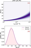 |
Fig. 1. Joint posterior distribution of magnetic field strength and electron density and marginal probability distribution of the magnetic field. Panel (A): Joint probability distribution of magnetic field strength and electron number density inferred for the average longitudinal oscillation period (Pl = 58 ± 15 min) reported by Luna et al. (2018), assuming uniform priors on electron density, 𝒰(ne,[cm−3]; 109, 1011) and magnetic field strength, 𝒰(B, [G];1, 70), evaluated on a 2D grid with Nne = 990 and NB = 1380 points. Panel (B): Marginal probability distribution of the magnetic field obtained from direct numerical integration (solid line) and from the emcee MCMC sampling (pink histograms), using a 2D parameter space with approximately 15 walkers, 50 000 steps per walker, and a burn-in phase discarding the first 20% of the iterations. |
The results obtained by direct integration over a grid of points are further validated with the use of MCMC sampling for the posterior distribution using the emcee algorithm (Foreman-Mackey et al. 2013). The methodology and application of the emcee algorithm is explained in Montes-Solís & Arregui (2017), Arregui et al. (2019), Baweja et al. (2024). In Figure 1(B), the pink histogram represents the results from MCMC sampling, and the solid line represents the direct integration result. Both approaches lead to very similar posteriors, which supports our obtained results.
The procedure was next applied to the two observations with simultaneous longitudinal and transverse oscillations reported by Mazumder et al. (2020) and Pan et al. (2025). The measured periods (Pl) for each case are shown in the second column of Table 1. The uncertainties in Pl are not given in Pan et al. (2025); thus, 10% uncertainty was assumed (Montes-Solís & Arregui 2019).
Longitudinal oscillation parameters and inferred magnetic field.
Additionally, based on the estimated values of B = 22.6 ± 11.9 G and B = 5.1 ± 0.5 G in Mazumder et al. (2020) and Pan et al. (2025), respectively, we can now construct more informed priors described by Equations (4) and (5), along with the uniform prior (Equation (3)). The marginal posterior distributions of B obtained for different priors and both studies are shown in Figure 2. The most probable values of B obtained from each prior and case are reported in Table 1.
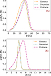 |
Fig. 2. Marginal posterior distributions of the magnetic field. Marginal probability distributions inferred using uniform (dot–dashed violet line), gamma (dashed orange line), and Gaussian (dotted teal line) magnetic-field priors from longitudinal oscillations in panels (A) Mazumder et al. (2020) and (B) Pan et al. (2025), with all distributions normalised to their maximum values. The direct solutions assume uniform priors on the electron number density, 𝒰(ne,[cm−3]; 109, 1011). For the magnetic field, the priors 𝒰(B, [G];1, 70), γ(B; 3.6, 0.2), and 𝒢(B, [G];22.6, 11.9) are used for panel (A), while 𝒰(B, [G];1, 70), 𝒢(B, [G];5.1, 0.5), and γ(B; 100, 20) are adopted for panel (B). |
From Figure 2, we find that for both observations and all prior types the marginal posterior distributions for the magnetic field strength can be well constrained. Differences in their shape and maximum a posteriori estimates exist depending on the prior used for the magnetic field strength. For the observation by Mazumder et al. (2020) (Figure 2(A)), the three posteriors are very similar and span almost identical ranges. For the observation by Pan et al. (2025) (Figure 2(B)), the posterior for the uniform prior is the least constrained, while the assumption of Gaussian and γ priors in B leads to almost identical posterior distributions.
Since the shape of the posterior depends on both the likelihood and the prior distribution – when a uniform prior is used – the posterior shape is primarily governed by the likelihood function. The likelihood depends on the mean and standard deviation of the measured periodicity of the longitudinal oscillations. The relative uncertainty in the periodicity reported by Luna et al. (2018) is about 25%, whereas it is around 10% and less than 1% for Pan et al. (2025) and Mazumder et al. (2020), respectively. The smaller the uncertainty in the period, the lower the joint probability p(B, ne|Pl, Ml). This explains why the posterior in Figure 1 resembles a Gaussian distribution, while those in Figure 2 (A) and (B) for the uniform prior case exhibit a sharper drop-off rate to the right of the maximum probability.
Furthermore, the relative uncertainties in the magnetic field values reported by Pan et al. (2025) and Mazumder et al. (2020) are 9.8% and 52.6%, respectively. Therefore, for Pan et al. (2025), the priors on B derived from both the gamma and Gaussian distributions are nearly similar, whereas for Mazumder et al. (2020), they differ significantly and thus more strongly influence the posterior shape. To verify this, we varied the uncertainty in B and found that as the uncertainty increases, the priors derived from the gamma and Gaussian distributions become increasingly different, leading to noticeable changes in the posterior. When the uncertainty in B is sufficiently large, the posterior distributions in Figure 2 (A) and (B) become more similar.
3.2. Inference of the length of the magnetic flux tube from transverse oscillations
After obtaining the probable magnetic field values, the next target was to estimate the length of the magnetic flux tube containing the prominence plasma from the seismology of the transverse oscillations. For this, we considered the prominence model for non-flowing prominence threads given by Díaz et al. (2002) and Dymova & Ruderman (2005). The equilibrium configuration of the filament is similar to that shown in Figure 7 of Mazumder et al. (2020). The length of the prominence thread is 2W, with a density ρp embedded in a magnetic flux tube of length 2L. The density of the evacuated parts of the flux tube is ρe, higher than that of the ambient corona ρc. The piecewise density along the flux tube is given by Equation 5 of Mazumder et al. (2020) and is similar to that in Dymova & Ruderman (2005). Díaz et al. (2002) and Dymova & Ruderman (2005) studied the normal modes of non-flowing filament threads (v0 = 0), whereas Terradas et al. (2008) did a similar seismological analysis for flowing threads (v0 ≠ 0). The results of Terradas et al. (2008) indicate that the flow effect is negligible, supporting the assumption of non-flowing threads and thereby validating our use of the model presented by Dymova & Ruderman (2005) in this analysis. Additionally, transverse oscillations are observed to occur in the same thread, which undergoes longitudinal oscillations in Mazumder et al. (2020). In Pan et al. (2025), the prominence undergoes both longitudinal and transverse oscillations simultaneously and from the slit positions (S3 and S4 in Figure 5 of Pan et al. 2025); it is assumed that the same thread undergoes simultaneous oscillations. Thus, the assumptions by Dymova & Ruderman (2005) are valid in these two studies. Further, in Dymova & Ruderman (2005), the system supports Alfvén and fast waves; however, the observed transverse oscillations result from the displacement of the cylindrical axis due to the kink-fast mode. Assuming thin tube approximation, Dymova & Ruderman (2005) provided the simple dispersion relation given by
 (12)
(12)
Here, Ω = ωL/vAc, e = ρe/ρc, c = ρp/ρc, l = W/L, vAc is the coronal Alfvén speed, ω is the oscillation frequency, and L is the half-length of the flux tube.
The density ratio e can take values between 0.6 and 2, as this range corresponds to the constant kink mode frequency (Dymova & Ruderman 2005). Moreover, for simplicity, it is considered to be unity, assuming that the evacuated region in the magnetic flux tube and the coronal environment have the same density. For fixed values of dimensionless variables c and l, Equation (12) seems to provide a unique solution for Ω. However, these dimensionless variables hide 5D variables (L, W, ρc, ρp, and vAc), and thus infinite solutions are possible. Utilizing the least positive root (Ω) of equation (12), substituting ω as 2π/pt in its relation with Ω, and rearranging it a bit to obtain the relation between pt and L in terms of Ω, we have
 (13)
(13)
Further, substituting for vAc in terms of the magnetic field and coronal density  in Equation (13), we obtain the model for the transverse oscillations (Mt) as:
 (14)
(14)
This equation serves as our model Mt and relates the length of the flux tube with the magnetic field strength and the period of the transverse oscillations. In what follows, we use pt and Pt to denote theoretical and observational transverse oscillation periods, respectively. Our model contains four relevant parameters, θt = {L, B, ρc, c}, once the length of the prominence threads (2W) is fixed. In Mazumder et al. (2020), the length of the prominence thread is reported to be 1.5 Mm, and for Pan et al. (2025), we estimated it to be 3 Mm. For three parameters L, ρc and c, we adopt uniform priors over reasonable ranges, i.e., 𝒰(L[Mm];50, 3000), 𝒰(ρc[kg m−3];10−14, 10−12), 𝒰(c; 5, 200). The posterior of B obtained from the analysis of longitudinal oscillations is now used as prior in Mt, thereby we have three different prior distributions for B (distribution of Bu, BG, and Bγ).
To construct the likelihood function, the smallest positive root of Equation (12) was used to calculate the modelled periods (pt), which were then compared with the observed periods (Pt) of the transverse oscillations. This likelihood function, along with the prior distribution of four parameters, yields a 4D posterior probability distribution. From this 4D posterior probability distribution, the joint probability distributions for magnetic field strength (B) and flux tube half-length (L), (p(B, L|Pt, Mt)), and for the flux tube half-length (L) and coronal density (ρc), (p(L, ρc|Pt, Mt)) were obtained.
A particular example result is shown in the upper two panels of Figure 3 for the oscillations observed by Mazumder et al. (2020). Additionally, the uncertainty in transverse oscillation periodicity is not reported, and thus 10% uncertainty is assumed to be associated with this parameter. The joint distributions indicate that both the magnetic field strength and the flux tube half-length can be well constrained. On the other hand, the coronal density cannot be properly inferred with the available information. The 2D joint probability distribution (p(B, L|Pt, Mt) was further marginalised to obtain the probable values of B and L, which are shown in the lower panels of Figure 3. Both posteriors are well-constrained, although the marginal posterior for the half-length of the flux tube displays a truncated long tail in the upper limit of our prior assumption. The direct integration results are validated by comparison with MCMC sampling of the posterior distribution using the emcee algorithm. Both approaches give similar results. The half-length is around 550 Mm; thus, the total length of the flux tube is 1100 Mm, which indicates that the quiescent prominences are longer than the active region prominences.
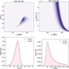 |
Fig. 3. Joint and marginal posterior distributions of flux-tube parameters. Top-left: Joint posterior distribution of magnetic field strength and flux-tube length. Top-right: Joint distribution of density and flux-tube length. Bottom-left: Marginal distribution of the magnetic field. Bottom-right: Marginal distribution of the flux-tube length, assuming uniform priors for all parameters and using the observational constraints of Mazumder et al. (2020). The prior on the magnetic field is taken from the posterior obtained in Sect. 3.1 using the uniform prior (Bu). The purple curves denote marginal posterior distributions obtained via Bayesian inference, while the pink histograms correspond to results from the emcee MCMC algorithm with the same dimensionality, number of walkers, steps, and burn-in phase as in Fig. 1. The bottom panels are not normalised 1. |
The inference was next applied to the transverse oscillations (Pt) observed in Mazumder et al. (2020) and Pan et al. (2025), using the different magnetic field distributions obtained in Section 3.1 to estimate the length of the prominences. The obtained results are shown in Figure 4, and the summary values are reported in Table 2. Again, 10% uncertainty was assumed in the periodicity of transverse oscillations.
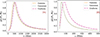 |
Fig. 4. Marginal probability distributions of the flux-tube length inferred using uniform (dot-dashed violet line), gamma (dashed orange line), and Gaussian (dotted teal line) magnetic-field priors from longitudinal oscillations in panels (A) Mazumder et al. (2020) and (B) Pan et al. (2025), with all distributions normalised to their maximum values. |
Transverse oscillation parameters and inferred flux-tube properties.
All inferred posteriors exhibit well-constrained distributions; thus, the method allows us to constrain the magnetic flux tube length from simultaneous observations of longitudinal and transverse oscillation. The posteriors display skewed profiles with long tails towards the upper regions of L, leading to larger upper uncertainties.
Notably, the inferred lengths for both events differ despite similar transverse oscillation periods, due to the marked difference in magnetic field strengths. Uniform priors yield posteriors shifted towards higher values of L, resulting in larger maximum a posteriori estimates, consistent with the trend seen when inferring magnetic field strengths from longitudinal oscillations. In their analysis, Mazumder et al. (2020) obtain a range of 2L ∈ [206 − 713] Mm. Our maximum posterior estimates are contained within that range.
3.3. Estimation of the twist number in flux tube
Quiescent prominences generally have inverse polarity configurations with respect to photospheric polarity (Leroy et al. 1984). According to this opposite polarity configuration, the prominence material lies in the twisted flux tubes (Kuperus & Raadu 1974). This configuration has been assumed in many models to explain the formation and the eruption of the prominences (van Ballegooijen & Martens 1989; Liakh et al. 2020; Zhou et al. 2023). Thus, assuming flux rope radius r and given the prominence length, we can estimate the number of twists (ϕ) of the flux rope where  . Here r is calculated from the longitudinal oscillation periodicity using Equation (8). To calculate ϕ, we considered the most probable length obtained for each distribution for each study, and the calculated twists are reported in Table 2. The number of twists in the flux rope reported in Mazumder et al. (2020) is also less than one, which matches our result using Bayesian inversion. As mentioned earlier, the length of the prominence estimated using a uniform prior of the magnetic field is greater than that for the other priors. Thus, the number of twists obtained for these priors also follows the same trend. Additionally, the comparatively higher twist number obtained for Pan et al. (2025) likely results from the assumption that the observed longitudinal and transverse oscillations occurred within the same prominence threads, although this was not explicitly stated in their study.
4. Conclusions
In this study, we employed the Bayesian inversion technique to infer physical parameters, such as the magnetic field strength and prominence length, by analysing the simultaneous longitudinal and transverse oscillations of the same prominences. We applied Bayesian prominence seismology to both wave modes, incorporating three prior distributions – uniform, gamma, and Gaussian. From longitudinal oscillations, we derived probable magnetic field strength, used as priors for posterior inference of magnetic flux tube length holding prominence plasma from transverse oscillations. Considering the flux rope model of the prominence magnetic structure, the number of turns in the associated flux tube was also estimated.
Since no single theoretical model currently exists that can simultaneously describe both longitudinal and transverse oscillations within the same prominence, we adopted two well-established models for our analysis. The pendulum model was employed to interpret the longitudinal oscillations, while the model proposed by Dymova & Ruderman (2005) was used for the transverse oscillations. Although these models differ in certain aspects, they share fundamental similarities. In the pendulum model, the prominence mass is assumed to be concentrated near the magnetic dip rather than filling the entire flux tube – an assumption consistent with the Dymova & Ruderman (2005) model as well. Therefore, the Bayesian approach adopted in this study remains valid under the assumption that both models appropriately represent different wave modes within the same magnetic flux tube.
In contrast to analytical seismological estimates, which provide either single-value estimates for the minimum magnetic field strength (Pant et al. 2016; Mazumder et al. 2020; Dai et al. 2021; Tan et al. 2023; Pan et al. 2025) or possible ranges of variation for the flux tube length (Mazumder et al. 2020), the Bayesian framework provides full probability distributions, conditional on the assumed models and observed data. It makes use of all the available information consistently and propagates uncertainty from observations to inferred parameters. Our direct integration results were validated by MCMC sampling of the posteriors.
The simplicity of the pendulum model makes inferring the magnetic field strength feasible, with accuracy that depends on our knowledge of the electron number density. A shortcoming is that Luna et al. (2022) estimated that for periods above ∼50 min, pendulum model predictions differ from those of models considering non-uniform gravity and non-circular dips.
Obtaining information about the length of the magnetic flux tube has traditionally been difficult. The most direct method involves estimating the length simply from the imaging observations of filaments. This approach has been considered in numerous studies (Vršnak et al. 2007; Shen et al. 2014). From transverse thread oscillation wavelengths in an active region prominence observed with Hinode, Okamoto et al. (2007) estimated a minimum flux tube length of 125 Mm. Montes-Solís & Arregui (2019) applied Bayesian inference to the same Hinode observations and obtained posteriors characterised by long and high tails. Their analysis suggests that the length of the flux tube can vary between 20 and 100 Mm.
The finest approach for estimating the flux tube length involves observing simultaneous transverse and longitudinal oscillations in the same prominence following the method of Mazumder et al. (2020). Their study assumed ranges for the magnetic field strength, density, and a fixed value of the coronal Alfvén speed, which yielded a range of possible values for L. Our study is the first to obtain full probability distributions for L with uncertainties propagated from observations to inferred values. These distributions are well constrained despite the large uncertainties, and future efforts should improve the inference accuracy.
Since no direct measurements of the length of field line exist, theoretical and numerical models (Liakh et al. 2020, 2021) depend on assumptions about the field lines being a few tens to hundreds of megametres long. From our study, it is clear that the length of the flux tubes holding the quiescent prominences can reach lengths from 100 Mm to 1000 Mm. Future observations capturing simultaneous longitudinal and transverse oscillations within the same prominence threads could enable reliable estimations of both the length and twist number for supporting magnetic flux tubes, and provide this information to more advanced numerical models.
Acknowledgments
The python code employed for the MCMC sampling of the posteriors in this study makes use of the emcee algorithm (Foreman-Mackey et al. 2013) and was developed upon an earlier version created by M. Montes-Solís. U.B. and V.P. express gratitude to ARIES for providing computational resources. I.A. acknowledges support from project PID2024-156538NB-I00 funded by MCIN/AEI/10.13039/501100011033 and by “ERDF A way of making Europe”. Finally, the authors would like to thank the referee for their valuable suggestions.
References
- Arregui, I. 2018, Adv. Space Res., 61, 655 [NASA ADS] [CrossRef] [Google Scholar]
- Arregui, I. 2022, Front. Astron. Space Sci., 9, 826947 [NASA ADS] [CrossRef] [Google Scholar]
- Arregui, I., & Asensio Ramos, A. 2011, ApJ, 740, 44 [NASA ADS] [CrossRef] [Google Scholar]
- Arregui, I., & Goossens, M. 2019, A&A, 622, A44 [NASA ADS] [CrossRef] [EDP Sciences] [Google Scholar]
- Arregui, I., Ramos, A. A., & Díaz, A. J. 2014, in Nature of Prominences and their Role in Space Weather, eds. B. Schmieder, J. M. Malherbe, & S. T. Wu, 300, 393 [Google Scholar]
- Arregui, I., Oliver, R., & Ballester, J. L. 2018, Liv. Rev. Sol. Phys., 15, 3 [Google Scholar]
- Arregui, I., Montes-Solís, M., & Asensio Ramos, A. 2019, A&A, 625, A35 [NASA ADS] [CrossRef] [EDP Sciences] [Google Scholar]
- Aschwanden, M. J. 2005, Physics of the Solar Corona. An Introduction with Problems and Solutions, 2nd edn. (Berlin, Heidelberg: Springer) [Google Scholar]
- Baweja, U., Pant, V., & Arregui, I. 2024, ApJ, 963, 69 [NASA ADS] [CrossRef] [Google Scholar]
- Dai, J., Zhang, Q., Zhang, Y., et al. 2021, ApJ, 923, 74 [NASA ADS] [CrossRef] [Google Scholar]
- Dai, J., Zhang, Q., Qiu, Y., et al. 2023, ApJ, 959, 71 [Google Scholar]
- Devi, P., Chandra, R., Joshi, R., et al. 2022, Adv. Space Res., 70, 1592 [NASA ADS] [CrossRef] [Google Scholar]
- Díaz, A. J., Oliver, R., & Ballester, J. L. 2002, ApJ, 580, 550 [Google Scholar]
- Dymova, M. V., & Ruderman, M. S. 2005, Sol. Phys., 229, 79 [Google Scholar]
- Dyson, F. 1930, MN, 91, 239 [Google Scholar]
- Engvold, O. 2000, in Encyclopedia of Astronomy and Astrophysics, ed. P. Murdin (Bristol: IOP) [Google Scholar]
- Foreman-Mackey, D., Hogg, D. W., Lang, D., & Goodman, J. 2013, PASP, 125, 306 [Google Scholar]
- Gilbert, H. R., Daou, A. G., Young, D., Tripathi, D., & Alexander, D. 2008, ApJ, 685, 629 [NASA ADS] [CrossRef] [Google Scholar]
- Gosain, S., & Foullon, C. 2012, ApJ, 761, 103 [Google Scholar]
- Hershaw, J., Foullon, C., Nakariakov, V. M., & Verwichte, E. 2011, A&A, 531, A53 [NASA ADS] [CrossRef] [EDP Sciences] [Google Scholar]
- Hyder, C. L. 1966, Z. Astrophys., 63, 78 [NASA ADS] [Google Scholar]
- Isobe, H., & Tripathi, D. 2006, A&A, 449, L17 [NASA ADS] [CrossRef] [EDP Sciences] [Google Scholar]
- Jing, J., Lee, J., Spirock, T. J., et al. 2003, ApJ, 584, L103 [NASA ADS] [CrossRef] [Google Scholar]
- Jing, J., Lee, J., Spirock, T. J., & Wang, H. 2006, Sol. Phys., 236, 97 [NASA ADS] [CrossRef] [Google Scholar]
- Joshi, R., Luna, M., Schmieder, B., Moreno-Insertis, F., & Chandra, R. 2023, A&A, 672, A15 [Google Scholar]
- Kleczek, J., & Kuperus, M. 1969, Sol. Phys., 6, 72 [NASA ADS] [CrossRef] [Google Scholar]
- Kucera, T. A., Luna, M., Török, T., et al. 2022, ApJ, 940, 34 [NASA ADS] [CrossRef] [Google Scholar]
- Kuperus, M., & Raadu, M. A. 1974, A&A, 31, 189 [NASA ADS] [Google Scholar]
- Labrosse, N., Heinzel, P., Vial, J. C., et al. 2010, Space Sci. Rev., 151, 243 [Google Scholar]
- Leroy, J. L., Bommier, V., & Sahal-Brechot, S. 1984, A&A, 131, 33 [Google Scholar]
- Li, T., & Zhang, J. 2012, ApJ, 760, L10 [NASA ADS] [CrossRef] [Google Scholar]
- Liakh, V., Luna, M., & Khomenko, E. 2020, A&A, 637, A75 [NASA ADS] [CrossRef] [EDP Sciences] [Google Scholar]
- Liakh, V., Luna, M., & Khomenko, E. 2021, A&A, 654, A145 [NASA ADS] [CrossRef] [EDP Sciences] [Google Scholar]
- Lin, Y., Soler, R., Engvold, O., et al. 2009, ApJ, 704, 870 [NASA ADS] [CrossRef] [Google Scholar]
- Liu, W., Ofman, L., Nitta, N. V., et al. 2012, ApJ, 753, 52 [NASA ADS] [CrossRef] [Google Scholar]
- Liu, R., Liu, C., Xu, Y., et al. 2013, ApJ, 773, 166 [NASA ADS] [CrossRef] [Google Scholar]
- Luna, M., & Karpen, J. 2012, ApJ, 750, L1 [NASA ADS] [CrossRef] [Google Scholar]
- Luna, M., Díaz, A. J., & Karpen, J. 2012, ApJ, 757, 98 [Google Scholar]
- Luna, M., Knizhnik, K., Muglach, K., et al. 2014, ApJ, 785, 79 [NASA ADS] [CrossRef] [Google Scholar]
- Luna, M., Su, Y., Schmieder, B., Chandra, R., & Kucera, T. A. 2017, ApJ, 850, 143 [NASA ADS] [CrossRef] [Google Scholar]
- Luna, M., Karpen, J., Ballester, J. L., et al. 2018, ApJS, 236, 35 [NASA ADS] [CrossRef] [Google Scholar]
- Luna, M., Terradas, J., Karpen, J., & Ballester, J. L. 2022, A&A, 660, A54 [NASA ADS] [CrossRef] [EDP Sciences] [Google Scholar]
- Mazumder, R., Pant, V., Luna, M., & Banerjee, D. 2020, A&A, 633, A12 [NASA ADS] [CrossRef] [EDP Sciences] [Google Scholar]
- Montes-Solís, M., & Arregui, I. 2017, ApJ, 846, 89 [Google Scholar]
- Montes-Solís, M., & Arregui, I. 2019, A&A, 622, A88 [NASA ADS] [CrossRef] [EDP Sciences] [Google Scholar]
- Ning, Z., Cao, W., Okamoto, T. J., Ichimoto, K., & Qu, Z. Q. 2009, A&A, 499, 595 [NASA ADS] [CrossRef] [EDP Sciences] [Google Scholar]
- Okamoto, T. J., Nakai, H., Keiyama, A., et al. 2004, ApJ, 608, 1124 [NASA ADS] [CrossRef] [Google Scholar]
- Okamoto, T. J., Tsuneta, S., Berger, T. E., et al. 2007, Science, 318, 1577 [Google Scholar]
- Oliver, R., & Ballester, J. L. 2002, Sol. Phys., 206, 45 [NASA ADS] [CrossRef] [Google Scholar]
- Oliver, R., & Murdin, P. 2001, in Institute of Physics Publishing, Bristol and Philadelphia, ed. P. Murdin, 3, 2707 [Google Scholar]
- Pan, W. W., Zhang, Q. M., & Qiu, Y. 2025, MNRAS, 542, 1308 [Google Scholar]
- Pant, V., Srivastava, A. K., Banerjee, D., et al. 2015, Res. Astron. Astrophys., 15, 1713 [Google Scholar]
- Pant, V., Mazumder, R., Yuan, D., et al. 2016, Sol. Phys., 291, 3303 [NASA ADS] [CrossRef] [Google Scholar]
- Ramsey, H. E., & Smith, S. F. 1966, AJ, 71, 197 [NASA ADS] [CrossRef] [Google Scholar]
- Roberts, B., Edwin, P. M., & Benz, A. O. 1984, ApJ, 279, 857 [CrossRef] [Google Scholar]
- Shen, Y., Liu, Y. D., Chen, P. F., & Ichimoto, K. 2014, ApJ, 795, 130 [Google Scholar]
- Soler, R., Oliver, R., & Ballester, J. L. 2011, ApJ, 726, 102 [NASA ADS] [CrossRef] [Google Scholar]
- Tan, S., Shen, Y., Zhou, X., et al. 2023, MNRAS, 520, 3080 [CrossRef] [Google Scholar]
- Tandberg-Hanssen, E. 1995, The Nature of Solar Prominences, 199 (Dordrecht: Springer) [Google Scholar]
- Terradas, J., Arregui, I., Oliver, R., & Ballester, J. L. 2008, ApJ, 678, L153 [NASA ADS] [CrossRef] [Google Scholar]
- Tripathi, D., Isobe, H., & Jain, R. 2009, Space Sci. Rev., 149, 283 [CrossRef] [Google Scholar]
- Uchida, Y. 1970, PASJ, 22, 341 [NASA ADS] [Google Scholar]
- van Ballegooijen, A. A., & Martens, P. C. H. 1989, ApJ, 343, 971 [Google Scholar]
- Vršnak, B., Veronig, A. M., Thalmann, J. K., & Žic, T. 2007, A&A, 471, 295 [NASA ADS] [CrossRef] [EDP Sciences] [Google Scholar]
- Yi, Z., & Engvold, O. 1991, Sol. Phys., 134, 275 [Google Scholar]
- Yi, Z., Engvold, O., & Keil, S. L. 1991, Sol. Phys., 132, 63 [NASA ADS] [CrossRef] [Google Scholar]
- Zhang, Q. M., Chen, P. F., Xia, C., & Keppens, R. 2012, A&A, 542, A52 [NASA ADS] [CrossRef] [EDP Sciences] [Google Scholar]
- Zhang, Q. M., Li, D., & Ning, Z. J. 2017, ApJ, 851, 47 [NASA ADS] [CrossRef] [Google Scholar]
- Zhang, Q. M., Guo, J. H., Tam, K. V., & Xu, A. A. 2020, A&A, 635, A132 [NASA ADS] [CrossRef] [EDP Sciences] [Google Scholar]
- Zhang, Y., Zhang, Q., Song, D. C., & Ji, H. 2024, arXiv e-prints [arXiv:2401.15858] [Google Scholar]
- Zhong, S., Hillier, A., & Arregui, I. 2025, ApJ, 991, 208 [Google Scholar]
- Zhou, Y., Ji, H., & Zhang, Q. 2023, Sol. Phys., 298, 35 [Google Scholar]
All Tables
All Figures
|
Fig. 1. Joint posterior distribution of magnetic field strength and electron density and marginal probability distribution of the magnetic field. Panel (A): Joint probability distribution of magnetic field strength and electron number density inferred for the average longitudinal oscillation period (Pl = 58 ± 15 min) reported by Luna et al. (2018), assuming uniform priors on electron density, 𝒰(ne,[cm−3]; 109, 1011) and magnetic field strength, 𝒰(B, [G];1, 70), evaluated on a 2D grid with Nne = 990 and NB = 1380 points. Panel (B): Marginal probability distribution of the magnetic field obtained from direct numerical integration (solid line) and from the emcee MCMC sampling (pink histograms), using a 2D parameter space with approximately 15 walkers, 50 000 steps per walker, and a burn-in phase discarding the first 20% of the iterations. |
| In the text | |
|
Fig. 2. Marginal posterior distributions of the magnetic field. Marginal probability distributions inferred using uniform (dot–dashed violet line), gamma (dashed orange line), and Gaussian (dotted teal line) magnetic-field priors from longitudinal oscillations in panels (A) Mazumder et al. (2020) and (B) Pan et al. (2025), with all distributions normalised to their maximum values. The direct solutions assume uniform priors on the electron number density, 𝒰(ne,[cm−3]; 109, 1011). For the magnetic field, the priors 𝒰(B, [G];1, 70), γ(B; 3.6, 0.2), and 𝒢(B, [G];22.6, 11.9) are used for panel (A), while 𝒰(B, [G];1, 70), 𝒢(B, [G];5.1, 0.5), and γ(B; 100, 20) are adopted for panel (B). |
| In the text | |
|
Fig. 3. Joint and marginal posterior distributions of flux-tube parameters. Top-left: Joint posterior distribution of magnetic field strength and flux-tube length. Top-right: Joint distribution of density and flux-tube length. Bottom-left: Marginal distribution of the magnetic field. Bottom-right: Marginal distribution of the flux-tube length, assuming uniform priors for all parameters and using the observational constraints of Mazumder et al. (2020). The prior on the magnetic field is taken from the posterior obtained in Sect. 3.1 using the uniform prior (Bu). The purple curves denote marginal posterior distributions obtained via Bayesian inference, while the pink histograms correspond to results from the emcee MCMC algorithm with the same dimensionality, number of walkers, steps, and burn-in phase as in Fig. 1. The bottom panels are not normalised 1. |
| In the text | |
|
Fig. 4. Marginal probability distributions of the flux-tube length inferred using uniform (dot-dashed violet line), gamma (dashed orange line), and Gaussian (dotted teal line) magnetic-field priors from longitudinal oscillations in panels (A) Mazumder et al. (2020) and (B) Pan et al. (2025), with all distributions normalised to their maximum values. |
| In the text | |
Current usage metrics show cumulative count of Article Views (full-text article views including HTML views, PDF and ePub downloads, according to the available data) and Abstracts Views on Vision4Press platform.
Data correspond to usage on the plateform after 2015. The current usage metrics is available 48-96 hours after online publication and is updated daily on week days.
Initial download of the metrics may take a while.