© The Authors 2026

1. Introduction

The Euclid Wide Survey (Euclid Collaboration: Mellier et al. 2025; Euclid Collaboration: Scaramella et al. 2022) will map the distribution of billions of galaxies up to redshift 2 across 14 000 deg² of the sky. This unprecedented new view of the Universe promises to further our understanding of the nature of dark energy and to test the assumptions of the standard model of cosmology, a universe dominated by a cosmological constant Λ and cold dark matter (ΛCDM).

For Euclid to deliver on these goals, it will require large-scale structure measurements that are made to a high precision and accuracy and are robust to observational systematic effects. In order to ensure these requirements are met, we will need to validate cosmological measurements against observational systematic effects. Critical for these validation studies are the construction of robust covariances that are independent of cosmological and galaxy bias assumptions. This will enable similar validation studies on weak-lensing measurements from the Kilo Degree Survey (KiDS; Heymans et al. 2021), Dark Energy Survey (DES; Abbott et al. 2022) Hyper Suprime-Cam (HSC; Hikage et al. 2019), following the validation studies of Ross et al. (2017) and Loureiro et al. (2022) on the Baryon Oscillation Spectroscopic Survey and KiDS, respectively. This will verify whether measurements are cosmological in origin and therefore ensure fundamental physics interpretations are reliable.

One of Euclid’s key science goals will be the measurement of clustering and cosmic shear angular power spectra from up to ten tomographic bins (Euclid Collaboration: Mellier et al. 2025), with 30 bins in multipole ℓ (between 10 ≤ ℓ ≤ 3000) for each auto and cross spectrum for clustering and weak-lensing E and B modes. With this setup, the full data vector is expected to be of the order of 10⁵ elements. Typical data-driven techniques for computing internal (i.e. from the data itself) or external covariances (i.e. from simulations) will be extremely demanding, both computationally and in terms of computing resources, such as storage. To ensure the covariances are non-singular, external covariances will require more than 10⁵ mocks, while internal covariances will require more than 10⁵ individual jackknife segments, as the number of mock or jackknife realisations needs to be greater than the length of the data vector. In practice, this requirement will likely be much higher, due to the need to reduce noise in the covariance estimates.

For cosmological measurements, it would seem appropriate to turn to analytic predictions (Alonso et al. 2019; García-García et al. 2019; Nicola et al. 2021); however, such methods will need to make explicit assumptions about the fiducial cosmology, galaxy population, and the survey (e.g. footprint) – assumptions that need prior validation and testing. For this reason we have been compelled to use data-driven internal estimates of the covariance matrix, which do no rely on such assumptions and can be relied on in cases where analytic predictions are not possible (such as for survey systematic effects). Furthermore, they allow us to estimate uncertainties critical for validation tests, such as testing for correlations with systematic effects via angular cross spectra where analytic covariance models do not exist.

For this paper, we estimated angular power spectrum covariances using jackknife resampling. Jackknife resampling techniques have been used in cosmology in the past, with a number of studies (such as Escoffier et al. 2016; Friedrich et al. 2016; Favole et al. 2021) finding them to be a reliable technique for covariance estimation. However, Norberg et al. (2009) cautioned the use of internal covariance estimates due to their tendency to be biased high (meaning the diagonals of the covariance are biased to larger values), while Shirasaki et al. (2017) and Lacasa & Kunz (2017) also raised concerns egarding covariances being underrepresented on large scales, the former due to scales similar to the jackknife regions and the latter as a result of failing to measure supersample covariances. Efron & Stein (1981) showed that jackknife covariances, overall, tend to be biased high – a property that can be removed by estimating the bias or through the computation of correction terms (Mohammad & Percival 2022). In this paper, we wish to establish a method for robustly measuring internal covariances using jackknife resampling that is both non-singular and unbiased and is capable of handling Euclid’s large data vector for angular power spectrum measurements of clustering and weak lensing.

The paper is organised as follows: in Sect. 2 we describe the construction of our Euclid-like lognormal galaxy catalogues; in Sect. 3 we describe a new method for creating jackknife segments on the sky; and in Sect. 4 the computation of angular power spectra, jackknife covariances, shrinkage, and bias removal. Furthermore, in Sect. 5 we explain how we tested the performance of our covariance estimates; in Sect. 6 we explain how we tested the accuracy of our covariance estimates; and, lastly, in Sect. 7 we summarise our findings and discuss future application to the Euclid Wide Survey.

2. GLASS simulations

We generate one thousand synthetic Euclid-like galaxy catalogues using GLASS (Tessore et al. 2023) – a package for generating galaxy catalogues from lognormal random fields. Lognormal fields, while not perfect, capture much of the rich covariance structure of real measurements (Hall & Taylor 2022), and allow us to quickly generate the large number of realisations that is necessary for characterising the population covariance. The simulations are designed to mimic the Euclid Wide Survey following a pre-launch definition of the wide-survey footprint. We assume a fiducial flat ΛCDM cosmology (Planck Collaboration VI 2020) with a Hubble constant H₀ = 67 km s⁻¹ Mpc⁻¹, matter density parameter Ω_m = 0.319, baryon density parameter Ω_b = 0.049, and a primordial power spectrum with an amplitude A_s = 2 × 10⁻⁹ and spectral index n_s = 0.96.

To ensure that the sample covariance is non-singular and the noise level is low, we limit the size of the data set to only two tomographic bins centred at redshifts z = 0.5 and z = 1, with each bin following a Gaussian redshift distribution with standard deviation 0.125. Furthermore, we adopt a constant galaxy bias of b_eff = 0.8 with a mean galaxy number density of 1 galaxy per arcmin² for each tomographic bin, approximately matching the number density of tomographic bins from the 13-bin Euclid survey setup (Euclid Collaboration: Mellier et al. 2025). Galaxy intrinsic ellipticities are assigned randomly with a standard deviation of 0.26 per ellipticity component before being corrected for weak lensing distortions. The catalogues are constructed from lognormal random fields generated in an ‘onion’ configuration with HEALPix maps at a resolution of NSIDE = 1024, similar to those used in Tessore et al. (2023).

To understand the expected results from the earliest Euclid data release we then cut the simulations to a pre-launch definition of the footprint for data release 1 (DR1; the first large data release from the first year of the wide survey), with the north region covering ≈1330 deg² (shown in Fig. 1) and the south ≈1260 deg² (shown in Fig. 2).

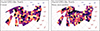Fig. 1. The jackknife partition segments shown for the North Euclid DR1-like wide survey footprint using the k-means method on the left and the binary space partitioning method on the right. Both maps have been divided into 151 segments, with each segment assigned a random colour for visibility. The maps are shown in an orthographic projection around the North polar cap.

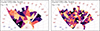Fig. 2. The jackknife partition segments shown for the South Euclid DR1-like wide survey footprint using the binary space partition method with 36 segments on the left and 144 on the right. Each segment has been assigned a random colour for visibility. The maps are shown in an orthographic projection around the South polar cap.

3. Sky partitioning

Delete-1 jackknife covariances are computed by partitioning the input data set into N_JK samples and running the analysis N_JK times, each with one of the N_JK samples removed. There are a number of ways data sets can be partitioned and resampled to compute jackknife covariances. In this analysis, we perform the partitioning at the map level, since this preserves spatial correlations and is a natural choice given the statistic of interest, angular power spectra, are computed from maps on the sky. This results in a spatial block jackknife. In cosmology, the sky partitioning is often carried out using a k-means clustering algorithm (e.g. see Kwan et al. 2017), which partitions the data set into N_JK clusters. Data points are members of the nearest cluster, creating a Voronoi cell partition structure. An example of the k-means partitioning is shown in the left panel of Fig. 1. This was performed using a k-means partitioning algorithm for the unit sphere¹. While this is a useful tool, the method has some computational drawbacks: firstly, the cluster finding algorithm is computationally intensive and secondly, and more critically, jackknife segments can have significant disparities in area. The area for each k-means jackknife segment, constructed from the Euclid DR1-like footprint, varies with a standard deviation of 16% from the mean. Jackknife samples are assumed to be equal and independent, but the extra variance in area means these regions cannot be treated as equal and depending on the statistics measured, could introduce significant extra area-dependent variance.

To tackle the drawbacks of k-means clustering, we develop a new method for partitioning the sky that applies the ‘binary space partitioning’ (BSP; Fuchs et al. 1980) algorithm on the unit sphere. BSP works by sequentially segmenting a polygon in any dimension along hyperplanes. For our specific requirements we take as input the survey footprint as a coverage map, given in HEALPix format (Górski et al. 2005), with values between 0 and 1. To compute a jackknife segmentation we first assign all pixels inside the footprint a jackknife segment ID of one and, to keep track of the number N_Seg of further subdivisions each segment needs to be divided into, we assign segment one an N_Seg = N_JK. Schematically, a single step in the sequential partitioning scheme works as follows:

1. Assuming the segment to be divided needs to be divided into N_Seg, we compute the weights of the two partitions to be

   $$\begin{array}{c}\hfill w_1=\frac{N_1}{N_{\mathrm{Seg}}}\mathrm{and}{w}_2=\frac{N_2}{N_{\mathrm{Seg}}},\end{array}$$(1)

   where

   $$\begin{array}{c}\hfill N_1=\lfloor \frac{N_{\mathrm{Seg}}}{2}\rfloor \mathrm{and}{N}_2=N_{\mathrm{Seg}}-N_1,\end{array}$$(2)

   and ⌊x⌋ is the floor function which rounds a number down to the nearest integer. This ensures the segment can be divided into an arbitrary number of segments rather than being limited to powers of two.

2. All points on the mask are expressed in angular coordinates (ϕ, θ) where ϕ ∈ [0, 2π) is a longitudinal angle and θ ∈ [0, π] the colatitude angle. We compute the barycentre of the segment by computing a weighted mean of the mask positions. This is carried out by first converting the coordinates of pixels in the mask into Cartesian coordinates r = (x, y, z) (assuming the points lie on a unit sphere) and computing the weighted mean

   $$\begin{array}{c}\hfill {\mathit{r}}_{\mathrm{barycentre}}=\frac{{\sum }_i{w}_i{\mathit{r}}_i}{{\sum }_i{w}_i},\end{array}$$(3)

   where the sum is over pixels in the mask and i denotes a specific pixel. The Cartesian barycentre is then converted into spherical polar coordinates.

3. We now rotate the mask so that the barycentre lies at the north pole of the unit sphere, denoting this new coordinate system as (ϕ′,θ′). We find the maximum θ′ of pixels in the mask in a wedge with width Δϕ′. The resolution needs to be fine enough to correctly measure the shape of the segment without being dominated by noise and becoming computationally intractable – in our analysis one hundred segments were used and this appears to be sufficient for both criteria (i.e. Δϕ = π/50). The longest side is taken to be

   $$\begin{array}{c}\hfill {\varphi }_{\mathrm{longest}-\mathrm{plane}}^{\prime }=\mathrm{argmax}\{{\theta }_{max}^{\prime }({\varphi }^{\prime })+{\theta }_{max}^{\prime }({\varphi }^{\prime }+\pi )\},\end{array}$$(4)

   where the function argmax finds the argument, in this case ϕ′ that maximises the function.

4. We perform another rotation to the plane of the longest side, which we will denote as (ϕ″, θ″), such that the line $\varphi {\prime }_{\mathrm{longest}-\mathrm{plane}}$ now lies on the line θ″ = π/2 and the centre of the points on the longest side lies at ϕ″ = π.

5. The segment is then divided along the longitudinal plane at $\varphi {″}_{\mathrm{div}}$ taken at one hundred steps between the minimum and maximum ϕ″ – with steps $\mathrm{\Delta }\varphi ″=({\varphi }_{max}″-{\varphi }_{min}″)/100$. On this first pass, the dividing hyperplane is taken to be the $\varphi {″}_{\mathrm{div}}$ where

   $$\begin{array}{c}\hfill {\varphi }_{\mathrm{div}}^{″}=\mathrm{argmin}\{\Vert \frac{w_1}{w_2}-\frac{{\sum }_{i,{\varphi }_i^{″}<{\varphi }_{\mathrm{div}}^{″}}w({\varphi }_i^{″})}{{\sum }_{i,{\varphi }_i^{″}>{\varphi }_{\mathrm{div}}^{″}}w({\varphi }_{\mathrm{i}}^{″})}\Vert \},\end{array}$$(5)

   searching for a dividing hyperplane that is closest to the intended balance w₁/w₂ for the two segments. The function argmin finds the argument, in this case ϕ″, that minimises the function. This step is repeated with a second pass which finds $\varphi {″}_{\mathrm{div}}$ more precisely by searching only in one hundred steps between $\varphi {″}_{\mathrm{div}}\pm 2\mathrm{\Delta }\varphi ″$.

6. Points in the segment with $\varphi ″>\varphi {″}_{\mathrm{div}}$ are assigned a new jackknife segment ID (one which is currently unassigned) with a N_Seg = N₂ while those with $\varphi ″\le \varphi {″}_{\mathrm{div}}$ retain their current segment ID with a new N_Seg = N₁.

This sequential partitioning repeats until all segments have N_Seg = 1. In Fig. 3 we show an illustrative explanation of the BSP algorithm. The partitioned map produced appears in sharp contrast to the Voronoi segments produced with k-means clustering (see Fig. 2), with the BSP producing segments that are trapezoidal or triangular in shape. Rather importantly, the BSP scheme resolves some of the limitations of k-means: firstly, by construction, the segment areas are kept very close to equal in area; and secondly the algorithm scales very well to larger maps (with higher resolution) and a larger number of partitions, typically taking 10% of the time. The segment areas from k-means vary significantly, with a standard deviation of 1.47 deg² (16% around the mean) for N_JK = 296, while for the binary space partition this is 0.01 deg² (0.11% around the mean) – a decrease in the standard deviation of roughly two orders of magnitude in comparison to k-means. This will minimise any uncertainties from variances in the area to any measured jackknife statistics. The BSP algorithm has been packaged into the public Python package SkySegmentor², allowing for the partitioning of either HEALPix maps or points on the unit sphere. Furthermore, if a mask contains many disjoint regions, SkySegmentor can be used to find and label the disjoint regions, so that they can be segmented individually.

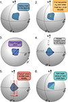Fig. 3. A schematic diagram displaying how the BSP algorithm was used to split a single region on the sky into two equal area segments.

In this paper we use several different jackknife partition maps, using the k-means and BSP methods with N_JK = 74, 148, 222 and 296 regions across the North and South Euclid DR1-like footprint. These numbers are chosen to minimise the area discrepancy between the segments in the North and South, which were partitioned individually. Partition maps for the South with N_JK = 36 and 144 are shown for the BSP method in Fig. 2. Note, that apart from the computational issues in constructing partition maps with k-means, we have found no difference in calculating jackknife covariances in the context of this paper and therefore have limited our discussion in this paper to the results from BSP.

4. Covariance estimation

In this section we detail the methods for computing angular power spectra for angular clustering and weak lensing from one thousand Euclid DR1-like catalogues. We then describe the techniques for estimating the sample covariance and computing jackknife covariance. Lastly, we describe the linear shrinkage and jackknife bias removal techniques used in this study.

4.1. Angular power spectra

Angular power spectra were computed using the techniques outlined in Euclid Collaboration: Tessore et al. (2025) which are available in the public python package Heracles³. We compute the auto and cross spectra C_ℓ for angular clustering (denoted with a P), and weak-lensing E and B modes (denoted with a E and B) for all tomographic bins (with the first bin denoted with a 0 and second with a 1). Note that we measure partial-sky angular power spectra here, and do not correct for the footprint. To ensure that at least some of the jackknife covariances (namely those with N_JK = 296) are not singular, we bin the angular power spectra into ten equal bins (whereas Euclid Collaboration: Mellier et al. 2025 provisionally use 30 bins) in logarithmic space in ℓ, between 10 ≤ ℓ ≤ 1024, resulting in a combined data vector with length 210. Modes below ℓ < 10 are ignored as they are dominated by cosmic variance and are poorly sampled with the Euclid DR1-like footprint, while modes beyond ℓ > 1024 go beyond the resolution of the GLASS simulations used to construct the mocks.

4.2. Sample covariance

The sample covariance is computed by first calculating the sample mean,

$$\begin{array}{c}\hfill {\overline{\mathit{C}}}_{\ell }^{f{f}^{\prime }}=\frac{1}{N_{\mathrm{S}}}{\displaystyle \sum _{i=1}^{N_{\mathrm{S}}}}{\mathit{C}}_{\ell ,i}^{f{f}^{\prime }},\end{array}$$(6)

where f and f′ denote specific maps or fields and in combination a specific auto- or cross-spectrum either between clustering P, or weak lensing E- or B-modes for tomographic bins 0 or 1. The subscript i denotes the C_ℓ computed from mock catalogue i from N_S samples. In our case this summation occurs across one thousand realisations (i.e. N_S = 1000). The sample covariance is computed as

$$\begin{array}{c}\hfill {\mathsf{C}}_{\mathrm{S}}^{f_1^{}{f}_1^{\prime }{f}_2^{}{f}_2^{\prime }}({\ell }_1,{\ell }_2)=\frac{1}{N_{\mathrm{S}}-1}{\displaystyle \sum _{i=1}^{N_{\mathrm{S}}}}({\mathit{C}}_{{\ell }_1,i}^{f_1^{}{f}_1^{\prime }}-{\overline{\mathit{C}}}_{{\ell }_1}^{f_1^{}{f}_1^{\prime }}){({\mathit{C}}_{{\ell }_2,i}^{f_2^{}{f}_2^{\prime }}-{\overline{\mathit{C}}}_{{\ell }_2}^{f_2^{}{f}_2^{\prime }})}^{\top },\end{array}$$(7)

where ⊤ denotes the transpose. In most cases we will drop the superscripts f and f′ and only use them when we are referring to a specific auto or cross spectrum, otherwise the reader can assume we are referring to the full data vector C_ℓ and full sample covariance matrix C_S. The sample covariance is treated as the ground truth covariance for this study.

4.3. Jackknife covariance

Jackknife covariances allow us to estimate the covariance directly from the data, without needing to make assumptions about the data, such as the cosmology and galaxy bias modelling. In this study, jackknife covariances are computed from a single simulation, and repeated for ten simulations – the latter to study the noise properties of the jackknife covariance in comparison to the sample covariance.

To compute the jackknife covariance, we must first create a set of jackknife samples. These are constructed by removing parts of the data and recomputing the C_ℓ. To do this we use the partition maps described in Sect. 3 and shown in Figs. 1 and 2, and compute the C_ℓ with galaxies in one of the jackknife segments removed. This is referred to as delete-1 jackknife samples, since only a single element is removed. In total this allows us to create N_JK jackknife samples C_ℓ, which we define as ${\mathit{C}}_{\ell }^{\mathrm{JK}}$, that we can use to compute an estimate of the covariance. We first compute the jackknife mean

$$\begin{array}{c}\hfill {\overline{\mathit{C}}}_{\ell }^{\mathrm{JK},f{f}^{\prime }}=\frac{1}{N_{\mathrm{JK}}}{\displaystyle \sum _{i=1}^{N_{\mathrm{JK}}}}{\mathit{C}}_{\ell ,i}^{\mathrm{JK},f{f}^{\prime }},\end{array}$$(8)

and then the jackknife covariance

$$\begin{array}{cc}\hfill {\mathsf{C}}_{\mathrm{JK}}^{f_1^{}{f}_1^{\prime }{f}_2^{}{f}_2^{\prime }}({\ell }_1,{\ell }_2)& =\frac{N_{\mathrm{JK}}-1}{N_{\mathrm{JK}}}{\displaystyle \sum _{i=1}^{N_{\mathrm{JK}}}}({\mathit{C}}_{{\ell }_1,i}^{\mathrm{JK},f_1^{}{f}_1^{\prime }}-{\overline{\mathit{C}}}_{{\ell }_1}^{\mathrm{JK},f_1^{}{f}_1^{\prime }})\hfill \\ \hfill & \times {({\mathit{C}}_{{\ell }_2,i}^{\mathrm{JK},f_2^{}{f}_2^{\prime }}-{\overline{\mathit{C}}}_{{\ell }_2}^{\mathrm{JK},f_2^{}{f}_2^{\prime }})}^{\top }.\hfill \end{array}$$(9)

This differs from Eq. (7) only by a jackknife prefactor (N_JK − 1)²/N_JK, meaning we can make use of standard covariance computation libraries, which assume independent samples, and then simply multiply the output by the jackknife prefactor.

4.4. Partial sky correction

In removing a portion of the data to compute the jackknife samples we are introducing a systematic bias caused by altering the footprints for the jackknife ${\mathit{C}}_{\ell }^{\mathrm{JK}}$. This is because the partial-sky C_ℓ computed in this analysis are affected by the survey footprint, unlike real space two-point correlation functions. Therefore the errors computed directly from the jackknife samples is not consistent with the measurements made with the full footprint. To correct the jackknife ${\mathit{C}}_{\ell }^{\mathrm{JK}}$ for the change in footprint we apply a correction for the difference in sky by transforming the angular power spectra into real space, analogous to the techniques employed in Szapudi et al. (2001) and Chon et al. (2004). To do this we also need to make a measurement of the angular power spectra for the footprint (used for clustering power spectra) and weight map (used for weak lensing power spectra) which we will refer to as M_ℓ for the entire footprint and ${\mathit{M}}_{\ell }^{\mathrm{JK}}$ for the jackknife samples. Converting from spherical harmonic space to real space requires the following transform

$$\begin{array}{c}\hfill C^{f{f}^{\prime }}(\theta )={\displaystyle \sum _{\ell }}\frac{2\ell +1}{4\pi }{C}_{\ell }^{f{f}^{\prime }}{d}_{s{s}^{\prime }}^{\ell }(\theta ),\end{array}$$(10)

where C(θ) is the real-space equivalent of the angular power spectra C_ℓ, d_ss′^ℓ is the Wigner D-matrix and s and s′ denote the spin weights of the field (0 for spin-0 fields such as the overdensity field and 2 for spin-2 fields such as the cosmic shear field). For a scalar fields (i.e. spin-0) this reduces to the Legendre polynomials. The inverse transform is given by

$$\begin{array}{c}\hfill C_{\ell }^{f{f}^{\prime }}=2\pi {\displaystyle {\int }_0^{\pi }}{C}^{f{f}^{\prime }}(\theta )d_{s{s}^{\prime }}^{\ell }(\theta )sin(\theta )\mathrm{d}\theta .\end{array}$$(11)

To account for the change in sky coverage caused by removing a jackknife region when computing ${\mathit{C}}_{\ell }^{\mathrm{JK}}$, we correct for the resulting mixing of harmonic modes – introduced by the altered footprint – by transforming to the real-space correlation function C_JK(θ). In real space, this mode coupling simplifies to a multiplicative correction involving the mask. Specifically, we apply the correction:

$$\begin{array}{c}\hfill {\stackrel{\sim }{\mathit{C}}}_{\mathrm{JK}}^{f{f}^{\prime }}(\theta )=\frac{{\mathit{M}}^{f{f}^{\prime }}(\theta )}{{\mathit{M}}_{\mathrm{JK}}^{f{f}^{\prime }}(\theta )}{\mathit{C}}_{\mathrm{JK}}^{f{f}^{\prime }}(\theta ),\end{array}$$(12)

where M(θ) and M_JK(θ) are the real-space analogues of the angular power spectra of the full-sky and jackknife footprint masks, respectively-that is, the real-space transforms of M_ℓ and M_ℓ^JK. We then convert ${\stackrel{\sim }{\mathit{C}}}_{\mathrm{JK}}^{ff\prime }(\theta )$ back to spherical harmonic space ${\stackrel{\sim }{\mathit{C}}}_{\ell }^{\mathrm{JK},ff\prime }$. However, this function is not stable when M_JK(θ)→0. To ensure M_JK(θ)→0 does not cause numerical instabilities, we force ${\stackrel{\sim }{\mathit{C}}}_{\mathrm{JK}}^{ff\prime }(\theta )\to 0$ when M(θ)→0. This is carried out by multiplying by a damping function

$$\begin{array}{c}\hfill {\stackrel{\sim }{\mathit{C}}}_{\mathrm{JK}}^{f{f}^{\prime }}(\theta )=\frac{{\mathit{M}}^{f{f}^{\prime }}(\theta )}{{\mathit{M}}_{\mathrm{JK}}^{f{f}^{\prime }}(\theta )}{\mathit{C}}_{\mathrm{JK}}^{f{f}^{\prime }}(\theta )f_{\mathrm{L}}\left({log}_{10}{\mathit{M}}_{\mathrm{JK}}^{f{f}^{\prime }}(\theta )\right),\end{array}$$(13)

where f_L is the logistic function

$$\begin{array}{c}\hfill f_{\mathrm{L}}(x,x_{\mathrm{L}},k_{\mathrm{L}})=\frac{1}{1+exp[-k_{\mathrm{L}}(x-x_{\mathrm{L}})]}.\end{array}$$(14)

The variables x_L and k_L have been set to x_L = −5 and k_L = 50; in effect this damps any signal where ${\mathit{M}}_{\mathrm{JK}}^{ff\prime }(\theta )<{10}^{-5}$. See Fig. 4 for a demonstration of the partial-sky correction to the pseudo C_ℓ.

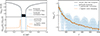Fig. 4. A demonstration of the partial-sky correction for the jackknife pseudo-Cℓ. In the top-left panel, the angular correlation function for the Euclid DR1-like mask (black) is compared to that of a single jackknife sample mask (blue). For angular scales between approximately 80° and 100°, no baselines are present in the footprint or the mask correlation function; this region is dominated by numerical noise. Since the jackknife footprint is slightly smaller, its mask correlation function contains fewer baselines in this range. In the bottom-left panel, we show the partial-sky correction function as the ratio of the full footprint to the jackknife footprint correlation functions (blue). The difference in baselines leads to significant noise in this correction function. This noise is mitigated by applying a logistic damping function (shown in orange). On the right, we illustrate the effect of applying a partial-sky correction directly to the jackknife Cℓ (blue), and compare it to a correction using the logistic damping function (orange). While a direct correction results in a very noisy angular power spectrum, the damped partial-sky correction yields a more robust and reliable estimate of the Cℓ.

4.5. Linear shrinkage

Estimates of the covariance from jackknife samples are often dominated by noise, a problem that can be alleviated by adding more samples and therefore more jackknife segments. While noisy estimates of the covariance are unbiased, the same is not true for its inverse and can lead to artificially tight parameter bounds (Hartlap et al. 2007; Sellentin & Heavens 2016). This is because the estimated covariance follows a Wishart distribution, which can be accounted for approximately through a bias correction (Hartlap et al. 2007; Percival et al. 2022) or more robustly at the likelihood level (Hotelling 1931; Sellentin & Heavens 2016). However, for Euclid’s very large data vector, in addition to a noisy covariance, any reasonable number of jackknife samples will result in a covariance that is singular. This means its usage will be limited to its diagonal components and will not be usable for any likelihood or complex analysis. To address this issue we apply linear shrinkage (Ledoit & Wolf 2004; Schäfer & Strimmer 2005; Pope & Szapudi 2008; Simpson et al. 2016; Looijmans et al. 2024), a technique used to dampen (or shrink) noise in an estimated covariance C_est by combining it with a well-conditioned target covariance C_tar, for instance one that is non-singular and not noise dominated,

$$\begin{array}{c}\hfill {\mathsf{C}}_{\mathrm{shr}}=\lambda {\mathsf{C}}_{\mathrm{tar}}+(1-\lambda ){\mathsf{C}}_{\mathrm{est}},\end{array}$$(15)

where λ is the linear shrinkage intensity and C_shr the shrunk covariance.

To compute the linear shrinkage intensity we must first compute the matrices

$$\begin{array}{c}\hfill {\mathsf{W}}_k({\ell }_1,{\ell }_2)=({\mathit{C}}_{{\ell }_1,k}-{\overline{\mathit{C}}}_{{\ell }_1}){({\mathit{C}}_{{\ell }_2,k}-{\overline{\mathit{C}}}_{{\ell }_2})}^{\top },\end{array}$$(16)

which we will use to estimate the variance of the covariance estimate. Note, the above computation assumes independent C_ℓ, if these are actually jackknife estimates ${\mathit{C}}_{\ell }^{\mathrm{JK}}$ then we multiply by the jackknife prefactor,

$$\begin{array}{c}\hfill {\mathsf{W}}_k({\ell }_1,{\ell }_2)=\frac{{(N_{\mathrm{JK}}-1)}^2}{N_{\mathrm{JK}}}({\mathit{C}}_{{\ell }_1,k}^{\mathrm{JK}}-{\overline{\mathit{C}}}_{{\ell }_1}^{\mathrm{JK}}){({\mathit{C}}_{{\ell }_2,k}^{\mathrm{JK}}-{\overline{\mathit{C}}}_{{\ell }_2}^{\mathrm{JK}})}^{\top }.\end{array}$$(17)

The mean of the matrix W_k is given by

$$\begin{array}{c}\hfill \overline{\mathsf{W}}=\frac{1}{N}{\displaystyle \sum _{k=1}^{N_{\mathrm{S}}}}{\mathsf{W}}_k,\end{array}$$(18)

which is related to the estimated covariance (sample or jackknife)

$$\begin{array}{c}\hfill {\mathsf{C}}_{\mathrm{est}}=\frac{N}{N-1}\overline{\mathsf{W}},\end{array}$$(19)

where N is the number of samples used to compute the estimate, either N_S for the sample covariance or N_JK for the jackknife covariance.

The covariance of the estimated matrix is generally defined as

$$\begin{array}{cc}\hfill \mathrm{Cov}({\mathsf{C}}_{\mathrm{est}}^{(ij)},{\mathsf{C}}_{\mathrm{est}}^{(xy)})& =\frac{N}{{(N-1)}^3}{\displaystyle \sum _{k=1}^N}({\mathsf{W}}_k^{(ij)}-{\overline{\mathsf{W}}}^{(ij)})\hfill \\ \hfill & \times ({\mathsf{W}}_k^{(xy)}-{\overline{\mathsf{W}}}^{(xy)}),\hfill \end{array}$$(20)

where the superscripts ij and xy denote two specific elements in the estimated covariance matrix. The variance for a single element ij in the covariance is given by

$$\begin{array}{c}\hfill \mathrm{Var}\left({\mathsf{C}}_{\mathrm{est}}^{(ij)}\right)=\mathrm{Cov}({\mathsf{C}}_{\mathrm{est}}^{(ij)},{\mathsf{C}}_{\mathrm{est}}^{(ij)}).\end{array}$$(21)

The optimal shrinkage intensity (Schäfer & Strimmer 2005) is generally given by

$$\begin{array}{c}\hfill {\lambda }^{★}=\frac{{\sum }_{i,j}[\mathrm{Var}\left({\mathsf{C}}_{\mathrm{est}}^{(ij)}\right)-\mathrm{Cov}({\mathsf{C}}_{\mathrm{tar}}^{(ij)},{\mathsf{C}}_{\mathrm{est}}^{(ij)})]}{{\sum }_{i,j}{({\mathsf{C}}_{\mathrm{tar}}^{(ij)}-{\mathsf{C}}_{\mathrm{est}}^{(ij)})}^2},\end{array}$$(22)

where we sum over all ij combinations (i.e. across all elements of the matrix) and λ^★ is a scalar. This specific form of shrinkage will be referred to as scalar shrinkage. However, we can compute the shrinkage intensity across blocks (unique combinations of auto- or cross-spectra, which we will refer to as block shrinkage) or without a summation at all and independently for each matrix element (referred to as matrix shrinkage). The form of Eq. (15) means that we must ensure that the shrinkage intensity λ lies in the range 0 ≤ λ ≤ 1, which we can carry out by setting

$$\begin{array}{c}\hfill \lambda =\{\begin{array}{cc}0,\hfill & {\lambda }^{★}<0,\hfill \\ {\lambda }^{★},\hfill & 0\le {\lambda }^{★}\le 1,\hfill \\ 1,\hfill & {\lambda }^{★}>1,\hfill \end{array}\end{array}$$(23)

where values of λ^★ below 0 and above 1, can occur due to noise.

In this paper we shrink towards a Gaussian correlation estimate, where the Gaussian prediction for the covariance is given by

$$\begin{array}{c}\hfill {\mathsf{C}}_{\mathrm{G}}^{f_1^{}{f}_1^{\prime }{f}_2^{}{f}_2^{\prime }}({\ell }_1,{\ell }_2)=({\stackrel{\sim }{\mathit{C}}}_{{\ell }_1}^{f_1^{}{f}_2^{}}{\stackrel{\sim }{\mathit{C}}}_{{\ell }_2}^{f_1^{\prime }{f}_2^{\prime }}+{\stackrel{\sim }{\mathit{C}}}_{{\ell }_1}^{f_1^{}{f}_2^{\prime }}{\stackrel{\sim }{\mathit{C}}}_{{\ell }_2}^{f_1^{\prime }{f}_2^{}}){\delta }_{\mathrm{K}}^{{\ell }_1{\ell }_2},\end{array}$$(24)

identity matrix given by I, the angular power spectra given by

$$\begin{array}{c}\hfill {\stackrel{\sim }{\mathit{C}}}_{\ell }^{f{f}^{\prime }}={\mathit{C}}_{\ell }^{f{f}^{\prime }}+\mathbf{I}·N^f{\delta }_{\mathrm{K}}^{f{f}^{\prime }},\end{array}$$(25)

the additive noise bias term given by N^f and ${\delta }_{\mathrm{K}}^{\mathit{ij}}$ the Kronecker delta function. The Gaussian covariance C_G therefore has a block-diagonal structure. We define the target covariance matrix as

$$\begin{array}{c}\hfill C_{\mathrm{tar}}^{\mathit{ij}}=\{\begin{array}{cc}{C}_{\mathrm{est}}^{(ii)},\hfill & i=j,\hfill \\ {\widehat{r}}_{\mathrm{G}}^{(ij)}\sqrt{C_{\mathrm{est}}^{(ii)}{C}_{\mathrm{est}}^{(jj)}},\hfill & i\ne j,\hfill \end{array}\end{array}$$(26)

and therefore shrink towards the correlation matrix of the Gaussian covariance ${\widehat{r}}_{\mathrm{G}}$, where ij are indices used to denote elements of the matrix,

$$\begin{array}{c}\hfill {\widehat{r}}_{\mathrm{G}}^{(ij)}=\frac{C_{\mathrm{G}}^{(ij)}}{\sqrt{C_{\mathrm{G}}^{(ii)}{C}_{\mathrm{G}}^{(jj)}}}·\end{array}$$(27)

We chose this target covariance for its simplicity and broad applicability to any angular power spectra measurements on the sphere, including systematics. Nevertheless, our method is general, and an alternative target covariance matrix may be used. Inserting Eq. (26) into Eq. (22),

$$\begin{array}{c}\hfill {\lambda }^{★}=\frac{{\sum }_{i\ne j}\mathrm{Var}\left(C_{\mathrm{est}}^{(ij)}\right)-{\widehat{r}}_{\mathrm{G}}^{(ij)}{f}^{(ij)}}{{\sum }_{i\ne j}{(C_{\mathrm{est}}^{(ij)}-{\widehat{r}}_{\mathrm{G}}^{(ij)}\sqrt{C_{\mathrm{est}}^{(ii)}{C}_{\mathrm{est}}^{(jj)}})}^2},\end{array}$$(28)

where

$$\begin{array}{c}\hfill f^{(ij)}=\frac{1}{2}(\sqrt{\frac{C_{\mathrm{est}}^{(jj)}}{C_{\mathrm{est}}^{(ii)}}}\mathrm{Cov}(C_{\mathrm{est}}^{(ii)},C_{\mathrm{est}}^{(ij)})+\sqrt{\frac{C_{\mathrm{est}}^{(ii)}}{C_{\mathrm{est}}^{(jj)}}}\mathrm{Cov}(C_{\mathrm{est}}^{(jj)},C_{\mathrm{est}}^{(ij)})),\end{array}$$(29)

closely following the maximum likelihood estimator for the Schäfer & Strimmer (2005) constant correlation target. As discussed previously, the shrinkage intensity is summed across the entire matrix for scalar shrinkage, across blocks for block shrinkage and without summation for matrix shrinkage – for the latter, diagonal components of the covariance are not shrunk (i.e. λ = 0).

4.6. Bias correction

Efron & Stein (1981) showed jackknife estimates of the variance tend to be biased high, which they proposed to remove with a delete-2 bias correction. In delete-2 jackknife samples, two jackknife segments are removed at a time, instead of the single segment removed in our original jackknife samples. This produces N_JK(N_JK − 1)/2 unique jackknife pairs and therefore comes at quite a significant computational cost. The corrected covariance, which we will refer to as the debiased jackknife, is computed from

$$\begin{array}{cc}& {\mathsf{C}}_{\mathrm{JK}}^{\mathrm{debias}}({\ell }_1,{\ell }_2)={\mathsf{C}}_{\mathrm{JK}}({\ell }_1,{\ell }_2)\hfill \\ \hfill & -\frac{1}{N_{\mathrm{JK}}(N_{\mathrm{JK}}+1)}{\displaystyle \sum _{i<i^{\prime }}}({\mathit{Q}}_{i{i}^{\prime }}({\ell }_1)-\overline{\mathit{Q}}({\ell }_1)){({\mathit{Q}}_{i{i}^{\prime }}({\ell }_2)-\overline{\mathit{Q}}({\ell }_2))}^{\top },\hfill \end{array}$$(30)

where

$$\begin{array}{c}\hfill {\mathit{Q}}_{i{i}^{\prime }}(\ell )=N_{\mathrm{JK}}{\mathit{C}}_{\ell }-(N_{\mathrm{JK}}-1)({\stackrel{\sim }{\mathit{C}}}_{\ell ,i}^{\mathrm{JK}}+{\stackrel{\sim }{\mathit{C}}}_{\ell ,i^{\prime }}^{\mathrm{JK}})+(N_{\mathrm{JK}}-2){\stackrel{\sim }{\mathit{C}}}_{\ell ,i{i}^{\prime }}^{\mathrm{JK}2}\end{array}$$(31)

and

$$\begin{array}{c}\hfill \overline{\mathit{Q}}(\ell )=\frac{2}{N_{\mathrm{JK}}(N_{\mathrm{JK}}-1)}{\displaystyle \sum _{i<i^{\prime }}}{\mathit{Q}}_{i{i}^{\prime }}(\ell ),\end{array}$$(32)

is the mean. In Eq. (31) the first C_ℓ is the angular power spectra from the entire footprint, ${\stackrel{\sim }{\mathit{C}}}_{\ell ,i}^{\mathrm{JK}}$ the delete-1 partial sky-corrected jackknife sample with segment i removed and ${\stackrel{\sim }{\mathit{C}}}_{\ell ,ii\prime }^{\mathrm{JK}2}$ the delete-2 partial sky-corrected debiased jackknife sample with segment i and i′ removed. The partial sky correction for the delete-2 jackknife sample are computed in the same way outlined in Sect. 4.4.

5. Performance

In this section we test the performance of our internal estimates of the covariance matrix from jackknife resampling. Furthermore, we explore the effects of partial sky correction, the dependence on jackknife sample number, linear shrinkage, and jackknife debiasing.

5.1. Dependence on partial sky correction

In Sect. 4.4 we explain how to correct the jackknife angular power spectra for differences in the footprint. To correct for the jackknife footprint we transform our data into real space to damp any signals where the correlations approach zero and would otherwise cause our correction to be numerically unstable. Partial-sky correction is crucial for correcting the mean of the angular power spectra but has little impact on the covariances which remain biased high with and without partial sky correction – a general property of covariance estimates from jackknife resampling Efron & Stein (1981). In Appendix A we discuss the effects of partial-sky correction in more detail.

5.2. Dependence on partition number

In Appendix B we discuss the relation between the number of jackknife partitions and the partial sky-corrected jackknife mean and standard deviation. For the mean, more partitions results in more accurate estimates of the angular power spectra, while the standard deviation (diagonals of the covariance) appears insensitive. The same is not true for the off-diagonal elements that appear to be strongly affected by the number of jackknife samples. In Fig. 5 we compare the correlation matrix of one realisation of the jackknife covariance matrix with N_JK = 74 and N_JK = 296 to the sample covariance. The off-diagonal components of the covariance follow a block diagonal structure, with strong correlations between angular power spectra typically only occurring at equal ℓ modes. Increasing the number of jackknife samples improves the off-diagonal structure of the covariance, at N_JK = 74 the off-diagonals are dominated by noise, while at N_JK = 296 the noise is suppressed and we can see more of the features shown clearly in the sample covariance. This fact is made clearer in Fig. 6 where we compare the eigenspectrum, the distribution of eigenvalues in the covariances (sorted from the largest eigenvalue to the smallest). Here we see a clear improvement in the covariance’s off-diagonal terms which more closely match that of the sample covariance as N_JK increases. The eigenspectrum is biased high for large eigenmodes, likely due to the bias towards larger diagonal components in the covariances shown in Fig. B.2.

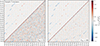Fig. 5. The correlation matrix shown in relation to the number of jackknife samples NJK (bottom right), in comparison to the sample covariance correlation matrix (top left corner). The correlation matrix is divided into blocks representing the covariance between each angular power spectra pair. On the left we show the jacknife covariances NJK = 74 and on the right with NJK = 296. Each angular power spectra is indicated with a label of the form XiYj where X and Y represent the angular power spectra type, either P for clustering or E and B for E- and B-modes, while the subscripts i and j represent the tomographic bin. Increasing NJK improves the non-diagonal structure of the jackknife covariance, features in the sample covariance start to show more clearly for NJK = 296 where the noise levels are lower.

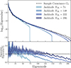Fig. 6. The eigenspectrum plotted as a function of the number of jackknife samples NJK (light to dark blue envelopes) in comparison to the sample covariance (dashed black line). In the bottom subplot we show the ratio with respect to the sample covariance. The solid lines represents the mean and the envelopes the spread (i.e. 95% confidence intervals) from ten realisations. Increasing NJK improves the off-diagonal structure of the jackknife covariance although we see a bias towards higher eigenvalues for the smaller eigenmodes. For NJK = 74 and 148 the covariance is singular, shown by the eigenspectrum dropping to zero for eigenmodes > NJK.

5.3. Shrinkage

In the previous section we have shown that the accuracy of the jackknife covariance, particularly off-diagonal components, significantly improves when more jackknife segments are used. However, for very large data vectors, of the order of 10⁵ elements, any reasonable number of jackknife samples (of the order of 10²) will produce a covariance that is singular (see Fig. 6). To address this issue we turn to shrinkage methods, which combine a noisy estimate of the covariance with a well-conditioned target covariance (see Sect. 4.5).

In Appendix C we consider several shrinkage methodologies, where the shrinkage intensity is either a single value (scalar shrinkage), a single value for each angular power spectra combination (block shrinkage), or a matrix where each component of the covariance is evaluate independently (matrix shrinkage). Scalar shrinkage is found to be the most accurate in general, while also being numerically stable. Therefore, we will only apply scalar shrinkage in the following parts of this paper.

In Appendix D we test the sensitivity of the shrinkage intensity λ to N_JK. We find that higher values of N_JK lead to λ estimates that are better constrained. This improves the precisions of the shrunk covariance although the covariance, still remains biased high, since shrinking towards a Gaussian correlation matrix does not alter the biased jackknife estimates of the standard deviation.

5.4. Bias correction

Up to this point we have seen that the diagonal components of the jackknife have tended to be biased high (see Figs. A.2 and B.2), an issue which cannot be resolved with our choice of shrinkage towards the correlation matrix. To address this limitation, in Sect. 4.6 we describe how to remove the jackknife bias with a method that uses delete-2 jackknife samples. In Fig. 7 we implement the delete-2 bias removal, and show the diagonal components for N_JK in relation to the sample covariance, demonstrating that the correction is able to remove the bias seen in the original jackknife covariance. However, at high-ℓ the bias for the auto spectra is slightly high, this appears to be correlated with the biases seen in the mean of the jackknife samples shown in Figs. A.1 and B.1.

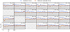Fig. 7. The standard deviation for the jackknife and debiased jackknife estimates of the covariance σJK, for NJK = 74, are compared to the sample covariance. The lines and error bars represent the mean and spread across ten realisations. See Fig. A.2 for details on the subplot layout. Debiasing removes the bias towards high diagonal components in the jackknife covariance.

In Fig. 8 we compare the original jackknife covariance with N_JK with scalar shrinkage and the debiased jackknife, showing that, although the debiasing is very good at correcting the diagonal components, the off-diagonals are very noisy. Noise appears to be concentrated at low ℓ. This is likely due to a breakdown of the jackknife assumptions; for instance the samples can be assumed to be independent, since low-ℓ measurements are highly correlated. This means we cannot use ${\mathsf{C}}_{\mathrm{JK}}^{\mathrm{debias}}$ by itself since the correlation structure is poor; see Fig. 9 showing the eigenspectrum that demonstrates this more clearly. To get the benefits of both methods, the unbiased diagonals of ${\mathsf{C}}_{\mathrm{JK}}^{\mathrm{debias}}$ and the correlation structure of C_shr, we combine the two in the following way

$$\begin{array}{c}\hfill {\mathsf{C}}_{\mathrm{DICES}}^{(ij)}=\frac{{\mathsf{C}}_{\mathrm{shr}}^{(ij)}}{\sqrt{{\mathsf{C}}_{\mathrm{shr}}^{(ii)}{\mathsf{C}}_{\mathrm{shr}}^{(jj)}}}\sqrt{{\mathsf{C}}_{\mathrm{JK}}^{\mathrm{debias},(ii)}{\mathsf{C}}_{\mathrm{JK}}^{\mathrm{debias},(jj)}}.\end{array}$$(33)

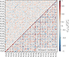Fig. 8. The correlation matrix of the jackknife covariance (top left) is compared to the same matrix after jackknife debiasing (bottom right). See Fig. 5 for details on the subplot layout. Debiasing produces a noisy covariance, especially in regions of low ℓ where the assumptions of the jackknife (i.e. that the samples can be treated as independent) break down. In contrast, linear shrinkage provides a covariance with lower noise-properties more closely matching the structure of the sample covariance correlation matrix.

This keeps the correlation structure of the shrunk covariance but replaces the diagonals with the debiased jackknife standard deviation. We call this technique DICES (Debiased Internal Covariance Estimation with Shrinkage). In Fig. 9 we compare the eigenspectrum of the sample covariance, in comparison to the shrunk covariance, debiased jackknife and DICES. The combination provides a covariance matrix with the correct off-diagonal structure as the sample covariance and removes the bias towards high eigenvalues seen in the ordinary jackknife while also removing the poor off-diagonal structure seen in the debiased jackknife. For this reason we advocate using DICES for internal covariances in future Euclid angular power spectrum measurement.

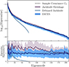Fig. 9. The eigenspectrum for jackknife shrinkage, debiased jackknife, and DICES (a combination of both with the jackknife shrinkage correlation structure with debiased jackknife standard deviation) computed from NJK = 74 and compared to the eigenspectrum of the sample covariance (dashed black line). In the bottom subplot we show the ratio with respect to the sample covariance. The solid lines represents the mean and the envelopes the spread (i.e. 95% confidence interval) from ten realisations. Linear shrinkage produces a covariance estimate that is non-singular but biased high, while the debiased jackknife is singular and has a poor non-diagonal structure. The combination resolves the deficiency of both methods, providing a covariance that is non-singular and unbiased.

6. Accuracy of internal covariance estimate

We test the accuracy of our covariance estimate using a cumulative signal-to-noise ratio (SNR),

$$\begin{array}{c}\hfill \mathrm{SNR}=\sqrt{{\mathit{C}}_{\ell }^{\top }{\mathsf{C}}^{-1}{\mathit{C}}_{\ell }},\end{array}$$(34)

where C is any estimate of the covariance matrix, or alternatively assuming all non-diagonal components are zero

$$\begin{array}{c}\hfill {\mathrm{SNR}}_{\mathit{diag}}=\sqrt{{\mathit{C}}_{\ell }^2·{\mathit{\sigma }}^{-2}},\end{array}$$(35)

where σ is a vector containing the square root of the diagonals of C. Computations of SNR are similar in form to a χ², used to compute a likelihood. Moreover, the SNR is equivalent to the Fisher information of a single global amplitude parameter, assuming Gaussian-distributed data (Tegmark et al. 1997). Therefore, the SNR weighs the covariance elements similarly to how they will be used in regression and inference.

In Fig. 10 we try to establish what aspect of the data vector dominates the measured SNR. We compute the SNR and SNR_diag for ten realisations with the corresponding shrunk jackknife covariance and DICES covariance. We carry this out by only including angular power spectra for clustering (i.e. P modes) and weak lensing E- and B-modes separately. Here we see that DICES for E- and B-modes is in both cases consistent with the sample covariance. On the other hand, the bias seen in clustering is removed when we use DICES. For the diagonal-only SNR_diag the values are biased low in both cases but the bias is improved with DICES. This illustrates that the covariance is strongly dependent on the accuracy of the clustering component. To balance the contributions between clustering and weak lensing E- and B-modes discussed below we limit the clustering angular power spectra to 10 ≤ ℓ ≤ 80, which provides a SNR of approximately 300.

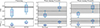Fig. 10. The SNR (top) and SNRdiag (bottom) broken down into the clustering (left), weak-lensing E-mode (middle), and B-mode (right) components. The SNR for jackknife shrinkage and DICES are shown. The dashed black line shows the mean and the grey envelopes the 95% confidence interval spread from ten realisations. The box-plot displays the full range with a vertical line, the box representing the interquartile range and the median indicated by a pink horizontal line. Replacing the standard deviations with the debiased jackknife diagonals improves the SNR and SNRdiag for clustering while for E and B-modes they are consistent with and without this correction. For SNRdiag the bias towards low values is seen only for clustering and improves with the corrected covariance but is not completely removed.

In Fig. 11 we compare SNR and SNR_diag for the joint clustering and weak lensing data vector computed with the sample covariance and the shrunk jackknife covariance as a function of N_JK. Increasing N_JK improves the precision of the covariance, leading to SNR with a smaller spread. For the full SNR this is always consistent with the sample covariance; however, when limited to only the diagonal components the SNR_diag is underestimated, due to the jackknife bias. In Fig. 12 we compare the SNR for the shrunk jackknife to DICES (i.e. C_DICES). Here we see that with the corrected diagonals the full SNR for DICES is biased slightly; however, the accuracy of SNR_diag improves when we use DICES instead of the shrunk covariance. This slight overestimation in the SNR is therefore likely caused by biases in the shrinkage estimation of the correlation matrix.

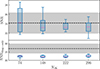Fig. 11. The SNR (top) and SNRdiag (bottom) for the joint clustering and weak-lensing data vector shown using the shrunk jackknife covariance as a function of NJK, relative to the sample covariance. Clustering spectra are limited to 10 ≤ ℓ ≤ 80 to balance contributions. Increasing NJK reduces the spread in both metrics. While SNR agrees with the sample covariance across all NJK, SNRdiag remains biased, though converging toward the sample estimate. See Fig. 10 for details.

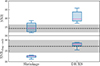Fig. 12. The SNR (top) and SNRdiag (bottom) for the joint clustering and weak-lensing data vector plotted for the jackknife shrinkage in comparison to DICES with NJK = 74. See Fig. 10 for details on the plot layout. To balance the contributions from clustering and weak lensing we limit all clustering auto and cross angular power spectra to 10 ≤ ℓ ≤ 80. Replacing the standard deviations with the debiased jackknife diagonals improves SNRdiag but biases SNR slightly high. This illustrates the bias is caused due to biases in the estimate of the correlation matrix.

To quantify the overall improvement in the covariance estimate, we measure the relative error (i.e. average fractional deviation) between elements of the estimated covariance to the sample covariance,

$$\begin{array}{c}\hfill \epsilon =\frac{{\sum }_{i,j}|{\mathsf{C}}_{\mathrm{est}}^{(ij)}-{\mathsf{C}}_{\mathrm{S}}^{(ij)}|}{{\sum }_{i,j}|{\mathsf{C}}_{\mathrm{S}}^{(ij)}|}·\end{array}$$(36)

Altogether, we find that DICES improves the deviations of the jackknife covariance by 33% and the jackknife correlation structure by 48%.

While in this paper we have only explored DICES with N_JK = 74 to keep computational cost down, we expect that the biases in SNR are due in part to the noisy estimates of the correlation matrix from such small jackknife samples, which will reduce when N_JK is increased.

7. Discussion

In this paper, we have developed a technique for computing accurate internal covariances for clustering and weak lensing angular power spectra. We call the method DICES, standing for Debiased Internal Covariance Estimation with Shrinkage, a combination of linear shrinkage of the correlation matrix and a debiased jackknife estimate. In Fig. 13 we outline the steps for computing the DICES internal covariance estimate, and in Fig. 14 we summarise its performance.

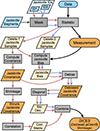Fig. 13. A schematic flow chart showing how to compute internal covariance estimates using DICES. Inputs are coloured in blue, while (internal) output products are coloured in (yellow) orange. Processes are coloured in grey. The red arrows indicate processes initiated with delete-1 jackknife samples, while blue arrows indicate processes involving delete-2 jackknife samples.

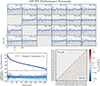Fig. 14. A summary of the performance of the internal covariance estimate DICES in comparison to the sample covariance. In the top panel we show the unbiased estimates of the standard deviation from DICES in comparison to the standard deviation of the sample covariance. On the bottom plots we compare DICES with the sample covariance showing that DICES reproduces an unbiased estimate of the eigenspectrum (left) and retains the correlation structure of the covariance (right).

In developing DICES we have outlined a new methodology for partitioning regions on the sky to high accuracy, a method based on applying the binary space partition algorithm (Fuchs et al. 1980) on the unit sphere and made publicly available in the SkySegmentor⁴ package. We have explored the dependence of jackknife covariance estimates on partial sky coverage and the number of jackknife samples, finding the former to have little to no impact on the covariance, while the off-diagonal structure of the covariance is significantly improved with increasing jackknife samples. We find scalar shrinkage, towards a Gaussian predicted correlation matrix, to produce reliable non-singular covariance estimates even for cases of large data vectors.

Finally, we estimate the jackknife bias via Efron & Stein (1981) that we use to compute a debiased jackknife covariance. We show that the diagonal standard deviations are consistent with the sample covariance, but the off-diagonals are dominated by noise. In combining the debiased jackknife covariance with the shrunk jackknife we are able to produce an internal covariance that is both debiased and with off-diagonals that are noise-reduced and consistent with the sample covariance.

In all cases we find that increasing the number of jackknife samples N_JK is always preferred. Even with shrinkage applied, the precision of the covariance improves with more jackknife samples. For this reason the Euclid Wide Survey should use as many jackknife samples as is computationally feasible. The main limitation is the computation of the jackknife bias, which requires the computation of N_JK(N_JK − 1)/2 jackknife samples. Since validation will require these covariances to be computed over many iterations, N_JK of order 100 will enable the computation to be made relatively fast while data release products could be produced with a much larger number of jackknife samples.

The DICES methodology outlined in this paper will enable robust measurements of the Euclid angular power spectra covariances directly from data, allowing for accurate angular power spectra covariances that are model-independent and for the measurement of systematic errors critical for validation. Both shrinkage and debiasing change the noise properties of the covariance matrix estimate, meaning neither the Hartlap et al. (2007) correction nor the Sellentin & Heavens (2016) likelihood correction can be applied. Future work could look towards improving our methodology, including understanding the small bias at high ℓ seen in the jackknife mean and jackknife covariances, the inclusion of E- and B-mode mixing during partial sky correction, and improvements in the covariance estimate at low ℓ where we expect the jackknife assumptions to break down (see Shirasaki et al. 2017; Lacasa & Kunz 2017). Furthermore, future analysis could explore the breakdown of some of the assumptions made in this paper-namely, that the summary statistics (angular power spectra) are dominated by Gaussian errors and noise, with non-Gaussian terms being small; and that the covariance matrices are parameter-independent. Fortunately, we find no evidence that these issues will drastically affect the covariance estimate, and therefore accurate internal covariances for Euclid DR1 will be possible using the DICES methodology. For future data releases, the increase in area will allow further optimisation of the shrinkage target, shrinkage intensity and the exploration of non-linear shrinkage (Joachimi 2017). The DICES methodology is made publicly available through the heracles.py⁵ package of the Euclid collaboration. A tutorial on how to implement the DICES methodology using the methods of heracles.py can be found here.

Acknowledgments

KN, NT, JRZ, and BJ acknowledge support by the UK Space Agency through grants ST/W002574/1 and ST/X00208X/1. AL acknowledges support by the Swedish National Space Agency (Rymdstyrelsen) through the Career Grant Project Dnr. 2024-00171. The Euclid Consortium acknowledges the European Space Agency and a number of agencies and institutes that have supported the development of Euclid, in particular the Agenzia Spaziale Italiana, the Austrian Forschungsförderungsgesellschaft funded through BMK, the Belgian Science Policy, the Canadian Euclid Consortium, the Deutsches Zentrum für Luft- und Raumfahrt, the DTU Space and the Niels Bohr Institute in Denmark, the French Centre National d’Etudes Spatiales, the Fundação para a Ciência e a Tecnologia, the Hungarian Academy of Sciences, the Ministerio de Ciencia, Innovación y Universidades, the National Aeronautics and Space Administration, the National Astronomical Observatory of Japan, the Netherlandse Onderzoekschool Voor Astronomie, the Norwegian Space Agency, the Research Council of Finland, the Romanian Space Agency, the State Secretariat for Education, Research, and Innovation (SERI) at the Swiss Space Office (SSO), and the United Kingdom Space Agency. A complete and detailed list is available on the Euclid web site (www.euclid-ec.org).

References

Appendix A: Mask correction

In Fig. A.1 we show that the partial-sky correction (measured for N_JK = 296) removes a bias in the jackknife sample mean. For the auto-spectra, the bias can be quite significant, but the correction generally mitigates this potential systematic error, leaving the jackknife mean to within 2% of the standard deviation of the original C_ℓ. However, there is a small systematic drop in the amplitudes at large ℓ for the auto-spectra which is not currently understood; however this offset is only seen in the mean (and is small, a < 2% offset) and does not impact the covariance estimate, discussed later. In Fig. A.2 we show the sky correction does not affect the covariance, which remains biased high with and without partial sky correction; this is a general property of covariance estimates from jackknife resampling (Efron & Stein 1981).

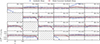Fig. A.1. The jackknife mean (${\overline{\mathit{C}}}_{\ell }^{\mathrm{JK}}$) before (in blue) and after (in red) correcting for the jackknife footprint is shown in comparison to the original angular power spectra computed for the entire footprint Cℓ. The lines and error bars represent the mean and spread across ten realisations. The difference is scaled as a function of the sample covariance standard deviation (σS i.e. the square root of the diagonals CS) with grey bands representing 2% standard deviations from the Cℓ for the entire footprint. The figure is divided into subplots for each angular auto and cross spectra pair, where P denotes overdensity, and E- and B-modes from weak lensing and the numbers 0 and 1 denote the tomographic bin. The sky correction is important for correcting the auto spectra for angular clustering but otherwise the correction has a minimal effect with the exception of a few cross-spectra (in particular P0 × E1).

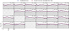Fig. A.2. The standard deviation for jackknife estimates of the covariance σJK (dashed horizontal grey line) before (in blue) and after (in red) correcting for the jackknife footprint is shown in comparison to the sample covariance standard deviation σS. The lines and error bars represent the mean and spread across ten realisations. The standard deviation for the jackknife covariance is unaffected by the sky correction.

Appendix B: Sensitivity to jackknife partition number

In Fig. B.1 we test the relation between the partial sky-corrected jackknife mean and the number of jackknife partitions N_JK, showing that on the whole the jackknife angular power spectra are unbiased, with the exception of the auto-spectra which show a damping at high ℓ. This damping reduces as the number of jackknife samples increases. The exact cause of this issue is unclear but is small, no more than 5% of the standard deviation. On the other hand, the cross-spectra are generally unbiased with the exception of the cross-spectra P0 × E1 (i.e. the correlation between the overdensity for the first tomographic bin with the E-modes of the second bin) which is biased high; again this is a small bias of no more than a few percent in comparison to the overall standard deviation. In Fig. B.2 we compare the diagonal components of the covariance as a function of the number of jackknife samples, showing that the jackknife standard deviation is robust to changes in the number of jackknife samples. In all cases we see that the jackknife standard deviation remains biased high in comparison to the sample covariance. Although the diagonal elements of the covariance are not dependent on N_JK for the values of N_JK studied, they will presumably be dependent for smaller N_JK.

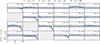Fig. B.1. The sky-corrected jackknife mean ${\overline{\mathit{C}}}_{\ell }^{\mathrm{JK}}$ is plotted as a function of the number of jackknife samples NJK. The lines and error bars represent the mean and spread across ten realisations. The difference is scaled as a function of the sample covariance standard deviation (σS i.e. the square root of the diagonals of CS). Increasing NJK improves the bias of the auto-spectra particularly at large ℓ, but except for a few cases (in particular P0 × E1), cross-spectra are generally unbiased for all NJK.

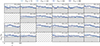Fig. B.2. The standard deviation for jackknife estimates of the covariance σJK is plotted as a function of the number of jackknife samples NJK in comparison to the sample covariance standard deviation σS. The lines and error bars represent the mean and spread across ten realisations. The number of jackknife samples does not appear to be changing the estimates of the diagonal components of the jackknife covariance.

Appendix C: Shrinkage method comparison

In Fig. C.1 we compare the jackknife covariance from N_JK = 74 with scalar shrinkage, block shrinkage, and matrix shrinkage. The methods differ in the way the shrinkage intensity is computed; for scalar shrinkage the shrinkage intensity λ is a single number estimated from the entire covariance matrix and is therefore the best constrained, for block shrinkage λ is evaluated for each block, and for matrix shrinkage λ is evaluated separately for each element of the matrix. The figure shows that in all cases the noise levels of the covariance are significantly reduced with linear shrinkage. However, for matrix shrinkage the noise levels appear to be enhanced and preserved for some elements, while block shrinkage dampens (i.e. moves towards zero) entire blocks of the covariance.

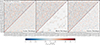Fig. C.1. The correlation matrix of the jackknife covariance with NJK = 74 (top left) is compared to the three different shrinkage methods: scalar shrinkage (left), block shrinkage (middle) and matrix shrinkage (right). See Fig. 5 for details on the subplot layout. In all case shrinkage dampens the noise-level of the covariance, however for matrix shrinkage this coupled with spurious noise.

In Fig. C.2 the eigenspectrum for each shrinkage method is compared to the eigenspectrum of the sample covariance. We show that in all cases shrinkage improves the off-diagonal structure of the covariance, with scalar shrinkage ensuring a non-singular well-conditioned matrix in all cases, block shrinkage is generally well conditioned but is singular in some cases (eigenmodes > 200 are close to zero), while matrix shrinkage (although better conditioned than the original jackknife covariance shown in Fig. 6) is singular for eigenmodes > 180 and starts to dip below the sample covariance at eigenmodes > 100. Methods for which the shrinkage intensity is computed from fewer summations, and which are therefore more localised (such as block and matrix shrinkage), have smaller uncertainties, while scalar shrinkage has fairly large uncertainties. This is likely due to the weaker damping of noise in scalar shrinkage in comparison to block and matrix shrinkage. However, since scalar shrinkage produces non-singular covariances in all cases, it is the most reliable and well conditioned. For this reason, in the rest of the paper we will only consider scalar shrinkage but future studies could consider improving the reliability of the other methods.

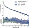Fig. C.2. The eigenspectrum for three shrinkage methods is compared to the sample covariance (dashed black line). Linear shrinkage is performed on the jackknife covariance with NJK = 74, using scalar, block, and matrix shrinkage. In the bottom subplot we show the ratio with respect to the sample covariance. The solid lines represent the mean and the envelopes the spread (i.e. 95% confidence interval) from ten realisations. Scalar shrinkage, with a single value for the shrinkage intensity, produces a covariance matrix that is non-singular and follows the sample covariance eigenspectrum for all eigenmodes, albeit with larger scatter. Block shrinkage is sometimes singular (eigenmodes > 200 are sometimes zero) while matrix shrinkage is always singular (eigenmodes > 180 are always zero). All methods are biased high for small eigenmodes, due to a bias towards high diagonals in the jackknife covariance which are not altered since we shrink towards a Gaussian correlation prediction.

Appendix D: Shrinkage sensitivity to jackknife partition number

In Fig. D.1 we compare the eigenspectrum of the shrunk covariance as a function of N_JK, showing that increasing the number of jackknife samples has a diminishing impact on the jackknife covariance estimate. However, the shrinkage intensity decreases and becomes better constrained (smaller variance) when N_JK increases. The increase in N_JK yields no noticeable difference in the eigenspectrum mean but improves the variance seen in the ten realisations and therefore improves the precision. We still see a bias in the eigenvalues which appears to originate from the bias in the standard deviation shown previously. Note that, since we shrink towards the correlation matrix of the Gaussian covariance expectation, the diagonals of the covariance will not change, meaning the bias towards higher standard deviations shown in Figs. A.2 and B.2 remains.

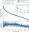Fig. D.1. The eigenspectrum for linear shrinkage as a function of NJK is compared to the eigenspectrum of the sample covariance (black dashed line). In the bottom subplot we show the ratio with respect to the sample covariance. The solid lines represents the mean and the envelopes the spread (i.e. 95% confidence interval) from ten realisations. In the inset subplot we show the mean and standard deviation for the scalar shrinkage intensity λ as a function of NJK, showing that increasing NJK leads to a smaller (non-zero) and better constrained λ. This more constrained λ leads to a more precise covariance, for instance the eigenspectrum shows less spread between realisations.

All Figures

	Fig. 1. The jackknife partition segments shown for the North Euclid DR1-like wide survey footprint using the k-means method on the left and the binary space partitioning method on the right. Both maps have been divided into 151 segments, with each segment assigned a random colour for visibility. The maps are shown in an orthographic projection around the North polar cap.
In the text

	Fig. 2. The jackknife partition segments shown for the South Euclid DR1-like wide survey footprint using the binary space partition method with 36 segments on the left and 144 on the right. Each segment has been assigned a random colour for visibility. The maps are shown in an orthographic projection around the South polar cap.
In the text

	Fig. 3. A schematic diagram displaying how the BSP algorithm was used to split a single region on the sky into two equal area segments.
In the text

Fig. 4. A demonstration of the partial-sky correction for the jackknife pseudo-Cℓ. In the top-left panel, the angular correlation function for the Euclid DR1-like mask (black) is compared to that of a single jackknife sample mask (blue). For angular scales between approximately 80° and 100°, no baselines are present in the footprint or the mask correlation function; this region is dominated by numerical noise. Since the jackknife footprint is slightly smaller, its mask correlation function contains fewer baselines in this range. In the bottom-left panel, we show the partial-sky correction function as the ratio of the full footprint to the jackknife footprint correlation functions (blue). The difference in baselines leads to significant noise in this correction function. This noise is mitigated by applying a logistic damping function (shown in orange). On the right, we illustrate the effect of applying a partial-sky correction directly to the jackknife Cℓ (blue), and compare it to a correction using the logistic damping function (orange). While a direct correction results in a very noisy angular power spectrum, the damped partial-sky correction yields a more robust and reliable estimate of the Cℓ.

In the text

Fig. 5. The correlation matrix shown in relation to the number of jackknife samples NJK (bottom right), in comparison to the sample covariance correlation matrix (top left corner). The correlation matrix is divided into blocks representing the covariance between each angular power spectra pair. On the left we show the jacknife covariances NJK = 74 and on the right with NJK = 296. Each angular power spectra is indicated with a label of the form XiYj where X and Y represent the angular power spectra type, either P for clustering or E and B for E- and B-modes, while the subscripts i and j represent the tomographic bin. Increasing NJK improves the non-diagonal structure of the jackknife covariance, features in the sample covariance start to show more clearly for NJK = 296 where the noise levels are lower.

In the text

Fig. 6. The eigenspectrum plotted as a function of the number of jackknife samples NJK (light to dark blue envelopes) in comparison to the sample covariance (dashed black line). In the bottom subplot we show the ratio with respect to the sample covariance. The solid lines represents the mean and the envelopes the spread (i.e. 95% confidence intervals) from ten realisations. Increasing NJK improves the off-diagonal structure of the jackknife covariance although we see a bias towards higher eigenvalues for the smaller eigenmodes. For NJK = 74 and 148 the covariance is singular, shown by the eigenspectrum dropping to zero for eigenmodes > NJK.

In the text

	Fig. 7. The standard deviation for the jackknife and debiased jackknife estimates of the covariance σJK, for NJK = 74, are compared to the sample covariance. The lines and error bars represent the mean and spread across ten realisations. See Fig. A.2 for details on the subplot layout. Debiasing removes the bias towards high diagonal components in the jackknife covariance.
In the text

Fig. 8. The correlation matrix of the jackknife covariance (top left) is compared to the same matrix after jackknife debiasing (bottom right). See Fig. 5 for details on the subplot layout. Debiasing produces a noisy covariance, especially in regions of low ℓ where the assumptions of the jackknife (i.e. that the samples can be treated as independent) break down. In contrast, linear shrinkage provides a covariance with lower noise-properties more closely matching the structure of the sample covariance correlation matrix.

In the text

Fig. 9. The eigenspectrum for jackknife shrinkage, debiased jackknife, and DICES (a combination of both with the jackknife shrinkage correlation structure with debiased jackknife standard deviation) computed from NJK = 74 and compared to the eigenspectrum of the sample covariance (dashed black line). In the bottom subplot we show the ratio with respect to the sample covariance. The solid lines represents the mean and the envelopes the spread (i.e. 95% confidence interval) from ten realisations. Linear shrinkage produces a covariance estimate that is non-singular but biased high, while the debiased jackknife is singular and has a poor non-diagonal structure. The combination resolves the deficiency of both methods, providing a covariance that is non-singular and unbiased.

In the text

Fig. 10. The SNR (top) and SNRdiag (bottom) broken down into the clustering (left), weak-lensing E-mode (middle), and B-mode (right) components. The SNR for jackknife shrinkage and DICES are shown. The dashed black line shows the mean and the grey envelopes the 95% confidence interval spread from ten realisations. The box-plot displays the full range with a vertical line, the box representing the interquartile range and the median indicated by a pink horizontal line. Replacing the standard deviations with the debiased jackknife diagonals improves the SNR and SNRdiag for clustering while for E and B-modes they are consistent with and without this correction. For SNRdiag the bias towards low values is seen only for clustering and improves with the corrected covariance but is not completely removed.

In the text

Fig. 11. The SNR (top) and SNRdiag (bottom) for the joint clustering and weak-lensing data vector shown using the shrunk jackknife covariance as a function of NJK, relative to the sample covariance. Clustering spectra are limited to 10 ≤ ℓ ≤ 80 to balance contributions. Increasing NJK reduces the spread in both metrics. While SNR agrees with the sample covariance across all NJK, SNRdiag remains biased, though converging toward the sample estimate. See Fig. 10 for details.

In the text

Fig. 12. The SNR (top) and SNRdiag (bottom) for the joint clustering and weak-lensing data vector plotted for the jackknife shrinkage in comparison to DICES with NJK = 74. See Fig. 10 for details on the plot layout. To balance the contributions from clustering and weak lensing we limit all clustering auto and cross angular power spectra to 10 ≤ ℓ ≤ 80. Replacing the standard deviations with the debiased jackknife diagonals improves SNRdiag but biases SNR slightly high. This illustrates the bias is caused due to biases in the estimate of the correlation matrix.

In the text

	Fig. 13. A schematic flow chart showing how to compute internal covariance estimates using DICES. Inputs are coloured in blue, while (internal) output products are coloured in (yellow) orange. Processes are coloured in grey. The red arrows indicate processes initiated with delete-1 jackknife samples, while blue arrows indicate processes involving delete-2 jackknife samples.
In the text

Fig. 14. A summary of the performance of the internal covariance estimate DICES in comparison to the sample covariance. In the top panel we show the unbiased estimates of the standard deviation from DICES in comparison to the standard deviation of the sample covariance. On the bottom plots we compare DICES with the sample covariance showing that DICES reproduces an unbiased estimate of the eigenspectrum (left) and retains the correlation structure of the covariance (right).

In the text

Fig. A.1. The jackknife mean (${\overline{\mathit{C}}}_{\ell }^{\mathrm{JK}}$) before (in blue) and after (in red) correcting for the jackknife footprint is shown in comparison to the original angular power spectra computed for the entire footprint Cℓ. The lines and error bars represent the mean and spread across ten realisations. The difference is scaled as a function of the sample covariance standard deviation (σS i.e. the square root of the diagonals CS) with grey bands representing 2% standard deviations from the Cℓ for the entire footprint. The figure is divided into subplots for each angular auto and cross spectra pair, where P denotes overdensity, and E- and B-modes from weak lensing and the numbers 0 and 1 denote the tomographic bin. The sky correction is important for correcting the auto spectra for angular clustering but otherwise the correction has a minimal effect with the exception of a few cross-spectra (in particular P0 × E1).

In the text

Fig. A.2. The standard deviation for jackknife estimates of the covariance σJK (dashed horizontal grey line) before (in blue) and after (in red) correcting for the jackknife footprint is shown in comparison to the sample covariance standard deviation σS. The lines and error bars represent the mean and spread across ten realisations. The standard deviation for the jackknife covariance is unaffected by the sky correction.

In the text

Fig. B.1. The sky-corrected jackknife mean ${\overline{\mathit{C}}}_{\ell }^{\mathrm{JK}}$ is plotted as a function of the number of jackknife samples NJK. The lines and error bars represent the mean and spread across ten realisations. The difference is scaled as a function of the sample covariance standard deviation (σS i.e. the square root of the diagonals of CS). Increasing NJK improves the bias of the auto-spectra particularly at large ℓ, but except for a few cases (in particular P0 × E1), cross-spectra are generally unbiased for all NJK.

In the text

Fig. B.2. The standard deviation for jackknife estimates of the covariance σJK is plotted as a function of the number of jackknife samples NJK in comparison to the sample covariance standard deviation σS. The lines and error bars represent the mean and spread across ten realisations. The number of jackknife samples does not appear to be changing the estimates of the diagonal components of the jackknife covariance.

In the text

	Fig. C.1. The correlation matrix of the jackknife covariance with NJK = 74 (top left) is compared to the three different shrinkage methods: scalar shrinkage (left), block shrinkage (middle) and matrix shrinkage (right). See Fig. 5 for details on the subplot layout. In all case shrinkage dampens the noise-level of the covariance, however for matrix shrinkage this coupled with spurious noise.
In the text

Fig. C.2. The eigenspectrum for three shrinkage methods is compared to the sample covariance (dashed black line). Linear shrinkage is performed on the jackknife covariance with NJK = 74, using scalar, block, and matrix shrinkage. In the bottom subplot we show the ratio with respect to the sample covariance. The solid lines represent the mean and the envelopes the spread (i.e. 95% confidence interval) from ten realisations. Scalar shrinkage, with a single value for the shrinkage intensity, produces a covariance matrix that is non-singular and follows the sample covariance eigenspectrum for all eigenmodes, albeit with larger scatter. Block shrinkage is sometimes singular (eigenmodes > 200 are sometimes zero) while matrix shrinkage is always singular (eigenmodes > 180 are always zero). All methods are biased high for small eigenmodes, due to a bias towards high diagonals in the jackknife covariance which are not altered since we shrink towards a Gaussian correlation prediction.

In the text

Fig. D.1. The eigenspectrum for linear shrinkage as a function of NJK is compared to the eigenspectrum of the sample covariance (black dashed line). In the bottom subplot we show the ratio with respect to the sample covariance. The solid lines represents the mean and the envelopes the spread (i.e. 95% confidence interval) from ten realisations. In the inset subplot we show the mean and standard deviation for the scalar shrinkage intensity λ as a function of NJK, showing that increasing NJK leads to a smaller (non-zero) and better constrained λ. This more constrained λ leads to a more precise covariance, for instance the eigenspectrum shows less spread between realisations.

In the text

References

- Abbott, T. M. C., Aguena, M., Alarcon, A., et al. 2022, Phys. Rev. D, 105, 023520 [CrossRef] [Google Scholar]
- Alonso, D., Sanchez, J., Slosar, A., & LSST Dark Energy Science Collaboration 2019, MNRAS, 484, 4127 [NASA ADS] [CrossRef] [Google Scholar]
- Chon, G., Challinor, A., Prunet, S., Hivon, E., & Szapudi, I. 2004, MNRAS, 350, 914 [Google Scholar]
- Efron, B., & Stein, C. 1981, Ann. Stat., 9, 586 [CrossRef] [Google Scholar]
- Escoffier, S., Cousinou, M. C., Tilquin, A., et al. 2016, arXiv e-prints [arXiv:1606.00233] [Google Scholar]
- Euclid Collaboration (Scaramella, R., et al.) 2022, A&A, 662, A112 [NASA ADS] [CrossRef] [EDP Sciences] [Google Scholar]
- Euclid Collaboration (Mellier, Y., et al.) 2025, A&A, 697, A1 [Google Scholar]
- Euclid Collaboration (Tessore, N., et al.) 2025, A&A, 694, A141 [Google Scholar]
- Favole, G., Granett, B. R., Silva Lafaurie, J., & Sapone, D. 2021, MNRAS, 505, 5833 [NASA ADS] [CrossRef] [Google Scholar]
- Friedrich, O., Seitz, S., Eifler, T. F., & Gruen, D. 2016, MNRAS, 456, 2662 [NASA ADS] [CrossRef] [Google Scholar]
- Fuchs, H., Kedem, Z. M., & Naylor, B. F. 1980, SIGGRAPH. Comput. Graph., 14, 124 [Google Scholar]
- García-García, C., Alonso, D., & Bellini, E. 2019, JCAP, 11, 043 [CrossRef] [Google Scholar]
- Górski, K. M., Hivon, E., Banday, A. J., et al. 2005, ApJ, 622, 759 [Google Scholar]
- Hall, A., & Taylor, A. 2022, Phys. Rev. D, 105, 123527 [NASA ADS] [CrossRef] [Google Scholar]
- Hartlap, J., Simon, P., & Schneider, P. 2007, A&A, 464, 399 [NASA ADS] [CrossRef] [EDP Sciences] [Google Scholar]
- Heymans, C., Tröster, T., Asgari, M., et al. 2021, A&A, 646, A140 [NASA ADS] [CrossRef] [EDP Sciences] [Google Scholar]
- Hikage, C., Oguri, M., Hamana, T., et al. 2019, PASJ, 71, 43 [Google Scholar]
- Hotelling, H. 1931, Ann. Math. Stat., 2, 360 [CrossRef] [Google Scholar]
- Joachimi, B. 2017, MNRAS, 466, L83 [NASA ADS] [CrossRef] [Google Scholar]
- Kwan, J., Sánchez, C., Clampitt, J., et al. 2017, MNRAS, 464, 4045 [NASA ADS] [CrossRef] [Google Scholar]
- Lacasa, F., & Kunz, M. 2017, A&A, 604, A104 [NASA ADS] [CrossRef] [EDP Sciences] [Google Scholar]
- Ledoit, O., & Wolf, M. 2004, J. Multivar. Anal., 88, 365 [Google Scholar]
- Looijmans, M. J., Wang, M. S., & Beutler, F. 2024, arXiv e-prints [arXiv:2402.13783] [Google Scholar]
- Loureiro, A., Whittaker, L., Spurio Mancini, A., et al. 2022, A&A, 665, A56 [NASA ADS] [CrossRef] [EDP Sciences] [Google Scholar]
- Mohammad, F. G., & Percival, W. J. 2022, MNRAS, 514, 1289 [NASA ADS] [CrossRef] [Google Scholar]
- Nicola, A., García-García, C., Alonso, D., et al. 2021, JCAP, 03, 067 [Google Scholar]
- Norberg, P., Baugh, C. M., Gaztañaga, E., & Croton, D. J. 2009, MNRAS, 396, 19 [Google Scholar]
- Percival, W. J., Friedrich, O., Sellentin, E., & Heavens, A. 2022, MNRAS, 510, 3207 [NASA ADS] [CrossRef] [Google Scholar]
- Planck Collaboration VI. 2020, A&A, 641, A6 [NASA ADS] [CrossRef] [EDP Sciences] [Google Scholar]
- Pope, A. C., & Szapudi, I. 2008, MNRAS, 389, 766 [NASA ADS] [CrossRef] [Google Scholar]
- Ross, A. J., Beutler, F., Chuang, C.-H., et al. 2017, MNRAS, 464, 1168 [Google Scholar]
- Schäfer, J., & Strimmer, K. 2005, Stat. Appl. Genet. Mol. Biol., 4, 32 [Google Scholar]
- Sellentin, E., & Heavens, A. F. 2016, MNRAS, 456, L132 [Google Scholar]
- Shirasaki, M., Takada, M., Miyatake, H., et al. 2017, MNRAS, 470, 3476 [NASA ADS] [CrossRef] [Google Scholar]
- Simpson, F., Blake, C., Peacock, J. A., et al. 2016, Phys. Rev. D, 93, 023525 [Google Scholar]
- Szapudi, I., Prunet, S., Pogosyan, D., Szalay, A. S., & Bond, J. R. 2001, ApJ, 548, L115 [Google Scholar]
- Tegmark, M., Taylor, A. N., & Heavens, A. F. 1997, ApJ, 480, 22 [NASA ADS] [CrossRef] [Google Scholar]
- Tessore, N., Loureiro, A., Joachimi, B., von Wietersheim-Kramsta, M., & Jeffrey, N. 2023, Open J. Astrophys., 6, 11 [NASA ADS] [CrossRef] [Google Scholar]