| Issue |
A&A
Volume 699, July 2025
|
|
|---|---|---|
| Article Number | A276 | |
| Number of page(s) | 16 | |
| Section | Galactic structure, stellar clusters and populations | |
| DOI | https://doi.org/10.1051/0004-6361/202555281 | |
| Published online | 17 July 2025 | |
Th/Eu abundance ratio of red giants in the Kepler field
1
Astronomical Science Program, Graduate Institute for Advanced Studies,
SOKENDAI, 2-21-1 Osawa,
Mitaka,
Tokyo
181-8588,
Japan
2
National Astronomical Observatory of Japan,
2-21-1 Osawa,
Mitaka,
Tokyo
181-8588,
Japan
3
Kapteyn Astronomical Institute, University of Groningen,
PO Box 800,
9700AV
Groningen,
The Netherlands
4
Astronomisches Rechen-Institut, Zentrum für Astronomie der Universität Heidelberg,
Mönchhofstraße 12-14,
69120
Heidelberg,
Germany
5
Kavli Institute for the Physics and Mathematics of the Universe (WPI), The University of Tokyo Institutes for Advanced Study, The University of Tokyo,
Kashiwa,
Chiba
277-8583,
Japan
★ Corresponding authors: This email address is being protected from spambots. You need JavaScript enabled to view it.
; This email address is being protected from spambots. You need JavaScript enabled to view it.
; This email address is being protected from spambots. You need JavaScript enabled to view it.
Received:
24
April
2025
Accepted:
5
June
2025
Abstract
The r-process production in the early Universe has been well constrained by extensive studies of metal-poor stars. However, the r-process enrichment in the metal-rich regime remains poorly understood. In this study, we examine the abundance ratios of Th and Eu, which represent the actinides and lanthanides, respectively, for a sample of metal-rich disk stars. Our sample covers 89 giant stars in the Kepler field with metallicities −0.7 ≤ [Fe/H] ≤ 0.4 and ages ranging from a few hundred million years to approximately 14 Gyr. Age information for this sample is available from stellar seismology, which is essential for studying the radioactive element Th. We derived Th and Eu abundances through χ2 fitting of high-resolution archival spectra (R ≈ 80 000) obtained with the High Dispersion Spectrograph at the Subaru Telescope. We created synthetic spectra for individual stars using a 1D local thermodynamic equilibrium spectral synthesis code, Turbospectrum, adopting MARCS model atmospheres. Our study establishes the use of a less extensively studied Th II line at 5989 Â, carefully taking into account the blends of other spectral lines to derive the Th abundance. We successfully determine the Eu abundance for 89 stars in our sample and the Th abundance for 81 stars. For the remaining eight stars, we estimate the upper limits of the Th abundance. After correcting the Th abundance for decay, we find no correlation between [Th/Eu] and [Fe/H], which indicates that actinide production with respect to lanthanide production does not depend on metallicity. On the other hand, we find a positive correlation of [Th/Eu] with age, with a slope of 0.10 ± 0.04. This may hint at the possibility that the dominant r-process sources are different between the early and late Universe.
Key words: stars: abundances / stars: atmospheres / stars: general / Galaxy: disk
© The Authors 2025
 Open Access article, published by EDP Sciences, under the terms of the Creative Commons Attribution License (https://creativecommons.org/licenses/by/4.0), which permits unrestricted use, distribution, and reproduction in any medium, provided the original work is properly cited.
This article is published in open access under the Subscribe to Open model. This email address is being protected from spambots. You need JavaScript enabled to view it. to support open access publication.
1 Introduction
Heavy elements (Z ≥ 30) in the Universe are produced by neutron-capture nucleosynthesis, an important part of which is the rapid neutron-capture process, known as the r-process (Burbidge et al. 1957; Cameron 1957). The r-process produces about half of the heavy elements, especially heavy elements with Z = 57-71 (the lanthanides), and exclusively elements with Z ≥ 90 (the actinides) (Seeger et al. 1965; Kratz et al. 1993; Goriely & Arnould 2001). For the r-process to occur, the physical conditions must satisfy a sufficiently high neutron density and a low electron fraction. Astrophysical sites that can host the r-process and reproduce the observed stellar abundance pattern are still under debate (Arnould et al. 2007; Kajino et al. 2019; Cowan et al. 2021). Among the proposed events are mergers of binary neutron stars (NSM) (Radice et al. 2018; Domoto et al. 2021; Naidu et al. 2022; Holmbeck et al. 2023), neutron star-black hole (NS-BH) mergers (Surman et al. 2008; Wehmeyer et al. 2019; Wanajo et al. 2024), and highly energetic cases of core-collapse supernovae (CCSNe) such as magnetorotational supernovae (MRD SNe) (Winteler et al. 2012; Cescutti & Chiappini 2014; Nishimura et al. 2017; Reichert et al. 2023). To date, NSMs are the only events proven to host the r-process, as observed from the electromagnetic counterparts of gravitational wave detections (Watson et al. 2019; Siegel 2022; Kasliwal et al. 2022; Domoto et al. 2025).
The abundances of r-process elements have been extensively studied in metal-poor stars, which are thought to have been polluted by a single r-process event (Truran 1981; Sneden et al. 1996; Farouqi et al. 2022). The abundance pattern of metalpoor stars can thus be used to infer r-process mechanisms as well as the astrophysical events and their physical properties. Europium, as an element with almost pure r-process contribution (Bisterzo et al. 2014), is usually used as a proxy for r-process study. On the other hand, Th is used as a proxy for actinides, as it has the isotope with the longest lifetime (14 Gyr). Another long-living actinide, U, is very difficult to detect as the absorption lines reside in the UV part of the stellar spectra and are very weak and often severely blended (Cayrel et al. 2001; Frebel et al. 2007; Placco et al. 2017; Shah et al. 2023). Studies of metal-poor stars revealed that, while elements from the second to the third r-process peak, including the lanthanides, follow a universal pattern (Sneden et al. 1996, 2000a; Westin et al. 2000; Honda et al. 2006), the actinides show variations: some stars exhibit overabundance or underabundance relative to the scaled solar pattern, termed actinide-boost and actinide-deficient stars, respectively (Cayrel et al. 2001; Hill et al. 2002; Honda et al. 2004; Placco et al. 2023). It is still debated whether this variation is caused by different r-process events or a variation in the same event (Schatz et al. 2002; Holmbeck et al. 2019; Wanajo et al. 2024). This highlights the importance of observing Th and Eu abundances, as they can help us understand the origin of r-process production, and especially the difference between lanthanides and actinides.
Understanding actinide production is crucial to the application of Th as an age indicator. The [Th/Eu] abundance ratios have been used as a chronometer to determine stellar ages (Sneden et al. 1996; Cowan et al. 1997; Honda et al. 2004; Frebel et al. 2007), as an alternative to isochrone methods, which are dependent on stellar evolution models. The caveat of using chronometers is the uncertainty in the theoretical initial production ratio (PR) of the elements involved, which contributes to the derived age uncertainty (Cayrel et al. 2001; Frebel et al. 2007). Once the PR is better constrained, the Th/Eu chronometer can provide more accurate age estimates.
While the studies of metal-poor stars provide valuable insights into the r-process production in the early Universe, the r-process enrichment in the more metal-rich region is less well understood. In contrast with metal-poor stars that are enriched by a single or minimum number of r-process sources, metal-rich stars contain a build-up of materials from several generations of star formation and r-process events (Reichert et al. 2021). The r-process event progenitors may evolve with time, resulting in different events dominating the metal-rich and metal-poor regimes. Thus, studying the r-process abundance in metal-rich stars is equally important for providing a complete picture of the r-process enrichment at a later stage and the evolution of the r-process with time.
In studying metal-rich stars, it is important to disentangle the r-process source(s) from that of other elements such as Fe and the α-elements. Previous studies of r-process abundances in metal-rich stars have found that the r-process and the α-elements show different evolutionary trends, suggesting different properties of supernovae that produce them (Guiglion et al. 2018). The number of contributing sources is also debated in the context of the timescale needed to produce the observed r-process abundance in metal-poor and metal-rich stars. Several studies found that two sources may be required to explain the observed abundance; these include one prompt source (e.g., MRD SNe) and one with a longer delay time (e.g., NSMs) (Wehmeyer et al. 2015; Côté et al. 2019; Kobayashi et al. 2020; Skúladóttir & Salvadori 2020; Tsujimoto 2021; Molero et al. 2023).
The origins of the r-process in disk stars are usually traced by the abundance of Eu, while the actinides are less widely studied. Recently, Th enrichment in disk stars has been studied by Mishenina et al. (2022), who compared the [Th/Fe] abundance trend with metallicities to predictions from galactic chemical evolution models. In studies of solar-type metal-rich stars as Mishenina et al. (2022), Th abundance is derived from the Th line at 4019 Â (del Peloso et al. 2005; Botelho et al. 2019). This line is widely used to determine Th abundances due to its detectability in solar-type stars. However, deriving Th abundances from this line is difficult because other atomic and molecular transitions contaminate the surrounding region. Some just overlap the Th line (e.g., Fe, Ni, Ce, Nd, Mn, and Co), with some weaker contributions from CH and CN. The Th abundance derived from this line is very sensitive to the estimate of the line strengths of these elements, especially for major blending components such as Fe, Ni, and Mn (Botelho et al. 2019). Therefore, an abundance analysis derived from a Th line with less severe contamination is desired to derive more accurate Th abundances.
An alternative approach is to utilize a Th line at 5989 Â, which is less blended compared to the one at 4019 Â. This line is known to provide a consistent Th abundance with those derived from other Th lines for an r-process-enhanced (RPE) very metalpoor giant star such as HD 221170 (Ivans et al. 2006). While this line is weak in non-RPE stars, it has been detected in the spectrum of Arcturus by Gopka et al. (2007) and further confirmed by Strassmeier et al. (2018). In such stars, the reliability of the Th abundance derived from this line has yet to be studied.
In this study, we investigated the evolution of Th and Eu abundances across different stellar ages and metallicities. For this purpose, we analyzed a sample of red giant stars in the Kepler field, which has prior information on stellar age from asteroseismology, allowing us to apply abundance corrections for Th decay and to study the relationship between its initial abundance, age, and metallicities. We focused on analyzing the Th 5989 Â line, examining the reliability of Th abundance measurements from this line. Our study provides a large sample of metal-rich stars with reliable Th abundances and age information.
Our study sheds new light on the evolution of Th and Eu in the metal-rich regime. We describe the data and methods in Sects. 2 and 3. We present the results and discussion in Sects. 4 and 5, and our conclusions in Sect. 6.
2 Data
Our sample consists of 89 giant stars, which is a combined sample from Takeda & Tajitsu (2015) and Takeda et al. (2016). The sample has seismic parameters (maximum frequency vmax and large separation frequency Δν) from NASA’s Kepler mission (Koch et al. 2010; Mosser et al. 2012). Takeda & Tajitsu (2015) determined the radii and masses using asteroseismic scaling relations with the seismic parameters determined by Mosser et al. (2012). Subsequently, Takeda et al. (2016) determined the age by assigning a stellar evolution model given the seismic mass and radius for each star. Liu et al. (2019) analyzed the same sample and determined the individual abundances of Na, Al, Mg, Si, Ca, Ti, V, Cr, Ni, Y, Ba, La, and Ce by comparing the observed equivalent widths with theoretical expectations based on the local thermodynamic equilibrium (LTE) model atmospheres by Kurucz (1993). They also determined the Eu abundance for 81 stars in the sample through the equivalent width (EW) method.
In this study, we derived our abundances using highresolution spectra obtained by Takeda & Tajitsu (2015) and Takeda et al. (2016). The data were originally taken on September 9, 2014, and July 3, 2015, using the High Dispersion Spectrograph (HDS, Noguchi et al. (2002) on the Subaru Telescope. The wavelength coverage is 5100-7800 Â, with a resolving power of R ≈ 80 000 and signal-to-noise ratio (S/N) of approximately 100-200 over the whole spectrum range, as reported in Takeda & Tajitsu (2015) and Takeda et al. (2016). We retrieved the reduced spectra from the Japanese Virtual Observatory portal for archive HDS spectra1.
We adopted the stellar parameters (Teff, log g, and [Fe/H]) derived by Takeda & Tajitsu (2015) and Takeda et al. (2016), given in Table A.1. They determined the stellar parameters by requiring the Fe abundances from individual Fe I and Fe II lines to show no dependence on excitation potentials and equivalent widths, as described in Takeda et al. (2002) and Takeda et al. (2005). We adopted the elemental abundances reported by Liu et al. (2019) in our analysis, except for Eu.
3 Methods
We derived the abundance ratios of Eu and Th through spectral synthesis methods based on model atmospheres. We created synthetic spectra with TSFitPy (Gerber et al. 2023; Storm & Bergemann 2023), the Python wrapper for Turbospectrum spectral synthesis code (Alvarez & Plez 1998; Plez 2012) with model atmospheres from an interpolation of MARCS model atmospheres (Gustafsson et al. 2008), assuming LTE conditions and 1D approximation (spherical symmetries for stars with low surface gravities and plane-parallel for stars with high surface gravities). We determined the best-fit abundance by χ2 minimization with the Nelder-Mead method, with the χ2 calculated as
 (1)
(1)
where Oi is the data point and Ei is the synthetic spectrum flux at the corresponding wavelength. The S/N was calculated locally from the noise around the continuum level near the analyzed Th and Eu lines. This typically falls in the range of S /N reported in Takeda & Tajitsu (2015) and Takeda et al. (2016), although sometimes lower or higher than the typical range.
We analyzed Arcturus as a standard star, adopting the following stellar parameters: Teff = 4286 ± 30 K, [Fe/H] = −0.52 ± 0.04, log g = 1.66 ± 0.05, and vmic = 1.74 kms−1 as determined by Ramírez & Allende Prieto (2011). We determined the Eu abundance using the Eu II line at 6645 Â, accounting for the hyperfine splitting (HFS) already included in the line list described in Sect. 3.1. The assumed Eu isotopic abundances are the default values set by Turbospectrum, i.e., the solar isotopic ratio (151Eu = 47.8% and 153Eu = 52.2%). The Th abundance is determined using the Th II line at 5989 Â. We adopted abundances of O, Na, Mg, Al, Si, K, Ca, Sc, Ti, V, Cr, Mn, Co, Ni, and Zn from Ramírez & Allende Prieto (2011). Of particular interest were the alpha elements, [Si/Fe] = 0.33 and [Mg/Fe] = 0.37, whose enhancement contributes to the continuum absorption. We also adopted typical Nd abundances for disk stars, [Nd/Fe] = 0.2 (Mishenina et al. 2013; Tautvaišiene et al. 2021) in the calculation of synthetic spectra for the Th line region. Since this Nd line is well separated from the Th line, it did not impact our Th measurement, although including this Nd abundance results in a better fit to the observation. We used this star as a reference to adjust the line list, as described in Sect. 3.1, and applied these adjustment to analyze our main sample.
For the main sample, we adopted the stellar parameters Teff, log g, and [Fe/H], estimated by Takeda & Tajitsu (2015) and Takeda et al. (2016). We also took into account individual elemental abundances from Liu et al. (2019), as mentioned above, and adopted [Nd/Fe] = 0.2 for the whole sample. We adopted the solar abundances from Asplund et al. (2009) to obtain the scaled solar abundances of Eu and Th.
3.1 Atomic and molecular line lists
We used the atomic line lists provided with the Turbospectrum code, based on the Gaia-ESO Survey (GES) line list (Ryabchikova et al. 2015; Heiter et al. 2021) with updated atomic data for C, N, O, Mg, and Si (Magg et al. 2022). The oscillator strength, log g f value of the Th line adopted in this study, was taken from the measurements of Nilsson et al. (2002). They reported a total uncertainty of 10% in the g f -value, which translates to an uncertainty of approximately 0.043 dex in log g f, and thus the same uncertainty in ATh. For comparison, the uncertainty of the g f -value for the Th II line at 4019 Â is 3% (log gf = −0.228 ± 0.013 Nilsson et al. 2002).
There are several absorption features around the region of the Th line causing potential blends, such as Si I lines toward blue at 5988.791 and 5988.838 Â (Fig. 1), an Nd II line toward red at 5989.378 Â, and a CN line overlapping with the Th line at 5989.054 Â. The line list predicts Si and Nd features that do not match the observed features. Hence, we made several adjustments to the line list to obtain a better match between the synthetic spectrum and the observation for Arcturus.
Adopting the Si abundance from Ramírez & Allende Prieto (2011), the synthetic spectra of the Si lines are too strong. As the Si abundance measurement of Ramírez & Allende Prieto (2011) is based on the analysis of five Si lines, we suspect this discrepancy to be caused by incomplete or incorrect atomic data of the two Si lines. The oscillator strengths of the two Si lines having the excitation potential of 5.964 eV originate from Robert L. Kurucz’s line list. As far as we know, there is no information on the reliability of these line data. As the original line list overestimates the strength of the Si I lines compared to the observed feature, we weaken the lines by gradually changing the oscillator strengths until the synthetic spectrum matches the observation. We changed the oscillator strength from log g f = −1.453 to log gf = −2.053 for the Si I line at 5988.791 Å. The Si I line at 5988.838 Å was neglected. As for the Nd line, we followed the adjustment made by Aoki et al. (2007), i.e., the wavelength, oscillation strengths, and excitation potential from 5989.378 to 5989.312 Å, log g f = −1.480 to −2.05, and χ = 0.745 eV to 0.38 eV. The final line list we adopted is shown in Table A.2.
We also included molecular line lists of two isotopes of CN (12C14N and 13C14N) compiled by Sneden et al. (2014), based on the transition data from Brooke et al. (2014), to fit the Eu line as well as additional 12C12C and TiO molecules from GES lists2 to fit the Th line. We further inspected the completeness of the CN line lists, especially 12C14N, which dominates over the other isotopes. In the online line list compiled by R. L. Kurucz3, two 12C14N lines that are absent from the list compiled by Sneden et al. (2014) are found at 5988.438 À and 5989.054 À. These are the transitions from J = 51.5 and J = 41.5, respectively, which exceed the range computed by Brooke et al. (2014). These lines are also tabulated on the VALD database4, based on the measurement by Kurucz, from which we confirmed the transition probabilities of the lines. Of particular interest is the line at 5989.054 À, which overlaps with the Th line under study. This line has an excitation potential of χ = 0.897 eV and oscillator strength of log gf = −2.23, according to Kurucz’s online database (see Table A.3).
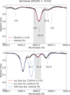 |
Fig. 1 Top panel: our fitting result of the Eu line for Arcturus. The dotted black line shows the observed spectrum; the solid red line shows the best-fit spectrum; and the dashed gray line shows the spectrum without Eu contribution. Bottom panel: our fitting result of the Th line in Arcturus. The dashed blue lines show the synthetic spectrum before the adjustment of the line list; the solid red line shows the final fitting result; and the dashed gray line shows the synthetic spectrum without Th contribution. |
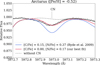 |
Fig. 2 CN line used to constrain the strength of CN absorption. The solid blue line indicates the synthetic spectrum assuming [C/Fe] and [N/Fe] from Ryde et al. (2009), while the solid red line indicates our best-fit result (see Sect. 3.2). The dashed gray line indicates the synthetic spectrum without CN contribution. |
3.2 CN line strength estimation
We examined the observed features of the aforementioned CN lines in Arcturus, assuming individual abundances of C and N from Ryde et al. (2009), [C/Fe] = 0.15 and [N/Fe] = 0.37. Our analysis included other CN lines belonging to the same vibrational transition of the same electronic system in the nearby regions, and the C and N abundances taken from the literature overestimated the strength of those lines. Therefore, we adjusted the C and N abundances using a 12C14N line that is not contaminated by atomic absorption. The CN line at 5972.985 À was suitable for this purpose (see Table A.3). We synthesized the spectra assuming several sets of C and N abundances to match the observed feature, as shown in Fig. 2. In this case, assuming [C/Fe] = 0.00 and [N/Fe] = 0.17 ([C + N/Fe] = 0.04), which we determined from the method described below, gives a better match to the observed feature. This is lower than the combined abundance of [(C + N)/Fe] = 0.20 presented in Ryde et al. (2009), which was derived from CN lines in the near-infrared region, whereas the lines we analyze lie in the optical region.
Based on the above discussion, we decided to independently estimate the 5989.054 Å CN line strength from the 5972.985 Å line instead of adopting C and N abundances from the literature. We note that our purpose is not to derive the C and N abundance but only to constrain the strength of the CN line to estimate the contamination on the Th line. For this purpose, we fit the 5972.985 Å CN line to determine N abundance while fixing the C abundance at [C/Fe] = 0.00. The C and N abundances assumed in the calculations for Arcturus are presented in Fig. 2. We adopted the best-fit [N/Fe] for the fixed [C/Fe] in the analysis of the Th line.
The final result of the adjustments of the Th line is shown in the bottom panel of Fig. 1. It is clear that the overall agreement between the synthetic and observed spectra is improved by updating the line list.
The Eu line is minimally blended with a CN line on the blue wing, as shown in the top panel of Fig. 1. There are multiple CN lines in this region, though most are very weak; the strongest are a 13C14N line at 6644.965 Å and 12C14N line at 6644.922 Å, according to the Brooke et al. (2014) line list. However, the contribution from 13C14N line is not identified in the current analysis.
Even though the blend is very weak in the case of Arcturus, the CN line is stronger in the case of more metal-rich stars (see Fig. 6). We estimate the strength of the CN line at 6644.922 Å using a CN line at 6644.304 Å (overlapping with another line at 6644.352 Å), which is directly adjacent to the Eu line (see Fig. 1). The blend on the Eu line slightly affects the Eu abundance determination in cool, metal-rich stars, as described in Sect. 4, where we find some discrepancy between our results and those of Liu et al. (2019). However, since the blend is located only on the wing of the Eu line, the Eu abundance is not very sensitive to the choice of the CN abundance, as long as the blend itself is included. The information on the CN lines used to constrain the strength and the CN lines contaminating the Th and Eu lines is given in Table A.3. We applied this method to our main sample. Fig. 3 shows the strength of the CN lines represented by their equivalent widths. It is evident that the strength of the CN lines increases with metallicity, indicating more prominent blends in more metal-rich stars.
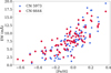 |
Fig. 3 Our estimate of the CN line strength (equivalent widths) derived by fixing the C abundance and varying N abundance. The strength of the CN line varies in the region of the Th and Eu lines, as indicated by the EW of the CN lines at 5972.985 and 6644.3 À. |
Typical uncertainties for Arcturus and our main sample.
3.3 Error estimation
The total error in the Th and Eu abundances stems from the stellar parameters, fitting, continuum placement, and the CN line contribution. To estimate the errors due to individual sources, we estimated the sensitivity of the Th and Eu abundances to changes in each parameter. As the Th line is blended with CN, we needed to separate the CN and Th contributions in estimating errors from stellar parameters, as the change in stellar parameters can also change the CN line contribution. We also estimated the sensitivity of Th abundances to the change of CN line strengths for a fixed set of stellar parameters. We applied the same treatment as for Th for the Eu line.
For our main sample, the intrinsic errors of the stellar parameters were estimated by Takeda & Tajitsu (2015) and Takeda et al. (2016) to be around 10-30 K for Teff, 0.05-0.1 dex for log g, 0.05-0.1 kms−1 for microturbulent velocity, and 0.02-0.04 dex for [Fe/H] (Takeda et al. 2008). Including the systematic difference from the stellar parameters in the Kepler Input Catalog (KIC), we estimated the errors of Teff, log g, vmic, and [Fe/H] to be 100 K, 0.1 dex, 0.2 km s−1, and 0.1 dex, respectively, following Liu et al. (2019). For Arcturus, we considered the uncertainties given by Ramírez & Allende Prieto (2011), 30 K for Teff, 0.05 dex for log g, and 0.04 dex for [Fe/H]. We did not consider the uncertainty from microturbulent velocity in Arcturus as it was not given by Ramírez & Allende Prieto (2011). The effect of microturbulent velocity was expected to be negligible, as demonstrated for our main sample. The typical uncertainties from stellar parameters for Th and Eu are given in Table 1.
Since we determined the abundance by χ2 fitting, we adopted the fitting error from the χ2 calculation. The abundance offset at 1σ was taken from the abundance for which the χ2 value is different by 1 from the best-fit value. We estimated continuum placement error by shifting the continuum level by 0.5% uniformly across the fitting window. We find that continuum error is one of the dominant contributors to the total error for Th, along with the fitting error.
We estimated the uncertainty of the strength of the 5989.054 Å CN line from the fitting and the continuum placement error of the 5972.985 Å line. The change in [Th/H] due to the error of the CN line strength varies from 0.0 to 0.1 dex in most cases, and up to approximately 0.3 dex in the most severe cases. On the other hand, even though the Eu line is blended with a CN line on the blue wing, the effect of the uncertainty of the CN line strength on the Eu abundance is less significant (see Table 1).
The total error is the sum of the individual sources of errors in quadrature. The errors of the Eu abundance are smaller than 0.1 dex in most cases, while the errors of Th vary significantly with the strength of the Th line and the S/N. There is no significant trend between stars with different ranges of stellar parameters for both Eu and Th, as the CN contributions are separated in estimating the errors from stellar parameters. In Table 1, we present three examples with varying Th line strength and S/N to illustrate their impact on the total uncertainty in the Th abundance. These three stars represent the best, typical, and worst cases regarding the Th line fitting quality. The total error is dominated by the fitting error, which is dependent on the S/N, and the continuum placement error, as shown in Table 1.
4 Results
4.1 Arcturus
The results of Eu and Th abundances for Arcturus are given in Table A.1 and shown in Fig. 4 with those for the main sample.
We compare our results with those of previous studies that use Arcturus as a standard star in their analysis. Worley et al. (2009) obtained [Eu/Fe] = 0.36 ± 0.04, which corresponds to [Eu/H] = −0.23, assuming their metallicity of [Fe/H] = −0.59 ± 0.12. Van der Swaelmen et al. (2013) found a value of [Eu/Fe] = 0.40 ± 0.05, corresponding to [Eu/H] = −0.25 assuming their metallicity of [Fe/H] = −0.65. The two literature results are in agreement with our result of [Eu/H] = −0.22 ± 0.04 within the uncertainty.
With the updated line list, we obtain [Th/H] = −0.34 or [Th/Fe] = 0.18. As far as we are concerned, the latest measurement of Th in Arcturus was done by Gopka et al. (1999), who reported log (Th) = −0.31 from two lines at 4510.526 Å and 4631.762 Å. Adopting the solar Th abundance from Asplund et al. (2009), this corresponds to [Th/H] = −0.33, in good agreement with our result. An earlier study by Holweger (1980) reported a value of [Th/H] = −0.90 obtained using the 4019 Å line. This result was derived by employing the oscillator strength from Corliss (1979), log gf = −0.19. A newer measurement by Nilsson et al. (2002) gives a value of log gf = −0.228. With the updated log g f , their abundance would correspond to [Th/H] = −0.862. This value is significantly lower than our result. As the 4019 Å line is more severely affected by blends, the Th abundance derived from this line is very sensitive to the contribution of the blending components. For example, Holweger (1980) assumed log gf = −2.60 for a blend by Co I line at 4019.126 Å, while a more recent value adopted by Mishenina et al. (2022) is log g f = −3.298. We suspect that the blending of the Co I line is overestimated in their analysis, which leads to an underestimation of the Th abundance.
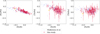 |
Fig. 4 From left to right: trend of [Eu/Fe], [Th/Fe], and [Th/Eu] against metallicities, respectively. The blue-filled circles show the results of Mishenina et al. (2022), and the red-filled circles show our results. The open red circles show the outliers discussed in the text, and the downward arrows denote upper limits. The yellow pentagon denotes Arcturus. |
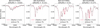 |
Fig. 5 Observed spectra of the Th line region (dots) compared to synthetic ones (lines). The fitting results of four stars in our sample with different metallicities show varying strengths of the CN line contribution. The solid red line shows the best-fit spectrum, and the dashed gray line shows the synthetic spectrum without Th contribution (i.e., the contribution from the CN line). The second left panel shows the case of the star with a high Th abundance, KIC4243623. |
4.2 Main sample
We successfully derive Eu abundances for all the stars in our sample. We derive the Th abundance for 81 stars in our sample, for which χ2 fitting reaches convergence. For the remaining 8 stars, in which the Th line is very weak or the feature is unclear, we estimate upper limits by searching for Th abundance that gives a line depth larger than the noise level. We show the bestfit spectra for four example stars with different metallicities in Figs. 5 and 6. The figures show that the contribution of the CN line varies with metallicity, both in cases of overlap with the Th line and with the blue wing of the Eu line.
The Th and Eu abundances for our sample are given in Table A.1. We show [Eu/Fe], [Th/Fe], and [Th/Eu] against metallicity in Fig. 4, along with the results from Mishenina et al. (2022) for comparison. We note that there are some outliers in our measurements that show low [Th/Fe] for their metallicities, KIC10382615 ([Th/Fe] = −0.15 at [Fe/H] = −0.49), KIC5858034 ([Th/Fe] = −0.25 at [Fe/H] = −0.19), and KIC4902641 ([Th/Fe] = −0.32 at [Fe/H] = 0.03). For KIC10382615, the Th feature is disturbed by noise, and for KIC5858034 and KIC4902641, we noticed a weak absorption feature, with a line depth less than 5%. This results in large fitting uncertainties for these stars, about 0.4 dex for KIC10382615 and KIC4902641, and 0.2 dex for KIC5858034. Taking into account the uncertainties, the three stars are not distinguished from the main trend of [Th/Fe].
We find one star with a high [Th/Fe], KIC4243623 ([Th/Fe] = 0.87 at [Fe/H] = −0.31). Since this star shows no discernible CN feature at 5972.985 A, we assume no contribution of CN. Even if we assume an upper limit for the CN contribution, i.e., [C/Fe] = 0.0 and [N/Fe] = 0.0, we still find a high value of [Th/Fe] ≈ 0.80 for this star. We also find a relatively high Eu abundance of [Eu/Fe] = 0.40. This star is regarded as an object with a slight enhancement in r-process elements. The observed and best-fit spectra for this star are shown in the second left panel of Figs. 5 and 6. Liu et al. (2019) classified this star to be a thin disk star, and it does not show any enhancements in other elements, for example, [Mg/Fe] = 0.18, [Ba/Fe] = −0.10, and [La/Fe] = −0.03. This finding is an interesting case where a metal-rich star exhibits such a high enhancement in r-process elements, especially Th (see Xie et al. 2024).
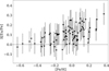 |
Fig. 7 Difference between [Eu/Fe] in Liu et al. (2019) and this study (Δ[Eu/Fe] = [Eu/Fe]literature - [Eu/Fe]this work). |
4.3 Comparison with previous studies
We analyze the same sample as Liu et al. (2019), who also report on [Eu/Fe] (see Fig. 7). The [Eu/Fe] values obtained by our analysis are lower than those from Liu et al. (2019) for the majority of stars in the sample. While we derive our abundance based on the spectral synthesis, Liu et al. (2019) relied on the measurement of the EW of the line, in which the blend with CN lines would not be taken into account. The discrepancy is larger for stars at higher metallicities, suggesting a more significant blend of the CN line. Although Liu et al. (2019) does not provide any information on the Eu lines they used to derive abundance, we suspect that the treatment of the blend of the CN line is the reason for this offset. Our findings for [Eu/Fe] align with the trend observed by Mishenina et al. (2022), as shown in the left panel of Fig. 4.
Our [Th/Fe] abundance trend is shown in the middle panel of Fig. 4 along with the results of Mishenina et al. (2022). The overall trend of our [Th/Fe] agrees with theirs, albeit with a slightly larger scatter around [Fe/H] ~ 0.0. This scatter is also found in the [Th/Eu] distribution in the right panel of Fig. 4. We discuss this scatter in more detail in Sect. 5.
We note that Mishenina et al. (2022) determined Th abundances for a sample of main-sequence stars from the 4019 A Th II line, which is significantly affected by the blending of multiple atomic and molecular features, the strongest being Fe. Therefore, some offset could arise between the Th abundances derived from the two lines if the treatment of blending is insufficient. Fig. 8 confirms that our [Th/Fe] shows no clear correlation with Teff, supporting that we were able to model the line and blending correctly.
To further test the consistency of Th abundances derived from both Th lines, we analyze a metal-poor giant star for which both lines are measurable, HD 221170. We do not find any significant offset between the results from the two lines in this star, with [Th/Fe] = 0.89 from both lines. This is in line with the study by Ivans et al. (2006), who showed an agreement of Th abundances derived from different lines. They found ATh = −1.49 from the Th II line at 5989 A and ATh = −1.46 from the line at 4019 A (Ivans et al. 2006). Therefore, we conclude that both Th lines give consistent abundances and the results are robust.
It should be noted, however, that comparing Th measurements from both lines as in the study by Ivans et al. (2006) is not possible for metal-rich stars. In main-sequence stars, the 5989 A line is too weak even at solar metallicity, while in metal-rich giants, the 4019 A line is not measurable because of severe contamination by other elements. Our sample and that of Mishenina et al. (2022) consist of stars at higher metallicities, where the effects of molecules can be important, rendering a direct comparison of Th abundance from both lines as in the case of HD 221170.
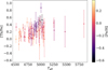 |
Fig. 8 [Th/Fe] distribution of the stars in our sample, color-coded according to metallicities. There is no correlation between the Th abundance and Teff or [Fe/H], supporting that our measurement is not affected by systematics in stellar parameters. |
4.4 NLTE effects
Our analysis adopts model atmospheres from the MARCS grids and the Turbospectrum spectral synthesis code, which assume 1D LTE conditions. The nonlocal thermodynamic equilibrium (NLTE) effects on Eu abundance have been studied for the 6645 A line with 1D model atmospheres (Guo et al. 2025). The correction is expected to be around 0-0.05 dex for red giants in our metallicity range, which is within our Eu abundance uncertainties. In the case of Th, Mashonkina et al. (2012) showed that there is a positive correction around 0-0.2 dex in cool stars for the 4019 A line, although there have not been any NLTE calculations to date for the 5989 A line. Although NLTE effects are not expected to be large for ionized lines such as the Th II line we use, future detailed NLTE calculations for this line would be of great interest to investigate the possible effects.
5 Discussions
This study presents the first determination of Th abundance from the 5989 A line, which has not been widely used previously, for a large sample of red giant stars. Our study demonstrates that the use of this line offers a new window to derive Th abundance in a larger number of stars.
The advantage of our sample is that ages are estimated by assigning stellar evolution models based on masses and radii derived from asteroseismic scaling relations. This enables us to correct the effect of decay of the actinide Th to obtain the initial abundance ratios. Due to radioactive decay, the currently observed Th abundance does not reflect the initial production of Th. Thus, examining the trend of initial Th abundance is more suitable to accurately infer the correlation between Th production with metallicities and ages.
We correct the Th abundance for the decay by adopting the stellar age provided by Takeda et al. (2016). The abundance of Th after time t decreases, according to the following equation:
 (2)
(2)
In the logarithmic scale of [Th/H], the difference between the initial and the current Th abundance is
![Mathematical equation: \rm{[Th/H]}_{\rm{initial}} - \rm{[Th/H]}_{\rm{now}} = \frac{\lambda t}{\ln(10)} = 2.15 \times 10^{-2} t/Gyr,](/articles/aa/full_html/2025/07/aa55281-25/aa55281-25-eq3.png) (3)
(3)
with t the stellar age in Gyr. Whereas the age uncertainty is not provided by Takeda et al. (2016), typical uncertainties from similar methods are 10-20% for red giants (Yu et al. 2018; Warfield et al. 2024; Pinsonneault et al. 2025). This would result in a change in age with an order of 0.07 dex in the logarithmic scale, and a 0.02 dex change in the Th abundance correction, which is smaller than our measurement uncertainty. Therefore, the impact of age uncertainty on the abundance trend is negligible compared to the uncertainty of abundance measurement.
In the discussion on the Th abundances corrected for the decay ([Th/H]initial from here onward), we assume that the r-process material was produced shortly before star formation. In reality, there might be some delay between the r-process production and star formation, and Th might have decayed during that period. Furthermore, accumulated Th from several r-process events might have decayed during the time between subsequent events.
5.1 [Eu/H] and [Th/H] trends with metallicities and ages
We first examine the possibility of different enrichment histories between stellar populations in our sample. Classifications into thin disk, thick disk, halo, or transition populations have been determined by Liu et al. (2019). Thin disk stars dominate our sample, with five thick disk, two halo, and two transition stars in the sample (see Table 4 of Liu et al. 2019). The only distinct difference is that the halo stars are of low metallicity, while the thick disk and transition stars overlap with thin disk stars in metallicities. Due to this distribution, we find no distinguishable difference in the trends of the abundance ratios between each population with our current sample.
Fig. 9 shows that age and metallicity do not exhibit a one-to-one relationship. Our sample can be divided into three groups: young metal-rich, old metal-rich, and old metal-poor stars, as indicated in the figure. As our sample covers stars with [Fe/H] ≥-0.7, there are no strictly “metal-poor” stars; the term is merely used to refer to stars with lower metallicity than the majority of the sample. Here we define metal-rich stars as those with [Fe/H] ≥ −0.1 and young stars as those younger than approximately 2 Gyrs of age. This is based on the borders of the region with no stars in the sample, located in the bottom left of Fig. 9.
The presence of the three groups is also visible in the [X/H] - [Fe/H] and [X/H] - age trends in Figs. 10 and 11. Examining abundance trends with age in terms of [X/Fe] may complicate the discussion because of the age-metallicity relation degeneracy. Thus, we examine the abundance trends in terms of [X/H] so as not to complicate the discussion of Eu and Th production with the variation of metallicity with age.
We fit a linear regression model to our data using the form
 (4)
(4)
where m is the slope and b represents the predicted value of y at x = xmean. This form ensures that the intercept is well-constrained without extrapolating beyond the data range while maintaining the robustness of the slope. We test the significance of the slope by the p-value, which indicates the probability of observing a trend when the null hypothesis of zero slope is true. Conservatively, a threshold of p = 0.05 is assumed to determine the significance of the trend. We show the p-value, slope, and the uncertainty of the slope for each of our linear regression fittings in Table 2.
Our result shows that [Eu/H] clearly correlates with metal-licity, as shown in the left panel of Fig. 10. The slope of [Eu/H] with [Fe/H] trend is significant compared to its uncertainty. The value of p = 0.0 confirms this result and, thus, we conclude that there is a significant correlation between [Eu/H] and [Fe/H].
On the contrary, we find that the correlation between [Eu/H] and age is less clear, close to a flat trend as shown on the left panel of Fig. 11. The linear fit shows a decreasing trend with increasing age, although the slope is not significant compared to the uncertainty. Indeed, we find a rather high p-value for the trend to be significant. Thus, our results suggest that [Eu/H] depends on metallicities rather than age. As found in the left panel of Fig. 11, old metal-poor stars have lower [Eu/H] than old metal-rich stars. Among them, four stars particularly have low values.
We identify the four old stars with the lowest [Eu/H] as KIC5737655 ([Eu/H] = −0.25 at [Fe/H] = −0.63), KIC6531928 ([Eu/H] = −0.25 at [Fe/H] = −0.57), KIC10382615 ([Eu/H] = −0.35 at [Fe/H] = −0.49), and KIC7734065 ([Eu/H] = −0.36 at [Fe/H] = −0.43). These stars have clear Eu line features, and the uncertainties indicate that our Eu measurement for these stars is robust.
We also examine the Th features of these stars. For KIC5737655 and KIC7734065, we successfully derive Th abundance and obtain [Th/H]initial = 0.20 and 0.35, respectively. KIC10382615 has a relatively large uncertainty and low [Th/Fe] deviating from the main trend in Fig. 4, as discussed in Sect. 4. We find [Th/H]initial = −0.47 for this star. We cannot derive Th for KIC6531928, and instead estimate an upper limit of [Th/H]initial = 0.13. As found in Fig. 11, [Th/H]initial of KIC5737655 and KIC7734065 do not deviate from the main trend with age, even though they show a deviation from the trend in [Eu/H]. The upper limit of Th for KIC6531928 also does not deviate from the trend, although we cannot make a definite judgment in this case. On the other hand, KIC10382615 shows both Eu and Th deviating from the trend, although the large uncertainty of Th for this star hinders us from making a clear conclusion on this matter. Interestingly, KIC5737655, KIC7734065, and KIC6531928 are classified into the thick disk by Liu et al. (2019), representing three out of five thick disk stars in the sample, while KIC10382615 is identified as a thin disk star. As these stars do not strongly deviate from the [Eu/H] - [Fe/H] correlation, their Eu abundance is consistent with the expectations for their metallicity range, particularly at the metal-poor end of the trend.
The [Th/H]initial trends are shown in the middle panel of Figs. 10 and 11. The correction in abundance is negligible for the youngest stars, while an increase in [Th/H] (and [Th/Eu]) reaches approximately 0.3 dex in the oldest stars. The impact of corrections is observable by comparing [Th/Eu]now and [Th/Eu]initial in Fig. 12 and the right panel of Fig. 11, respectively. In Fig. 12, the oldest stars show quite low [Th/Eu]now compared to the young stars but show higher [Th/Eu]initial after correction for the decay.
We exclude upper limits and the three stars with the lowest [Th/H], which have large uncertainties discussed in Sect. 4, from our linear regression fittings. To ensure the robustness of our analysis, we also examine the trends excluding the stars with total Th abundance uncertainties larger than 0.3 dex. The slopes of the [Th/H]initial and [Th/Eu]initial trends with ages and metallicities exhibit little to no change. This does not change the significant correlations described below.
We find a significant correlation between [Th/H]initial and metallicity, as shown in the middle panel of Fig. 10. On the other hand, no significant correlation between [Th/H]initial and age is found in the middle panel of Fig. 11. This suggests that [Th/H]initial, similarly to [Eu/H], depends on metallicities rather than ages.
No significant correlation is found between [Th/Eu]initial and metallicity, as shown in the right panel of Fig. 10. In Sect. 4, we point out that [Th/Eu]now exhibits a large scatter in the metal-rich region ([Fe/H] ≥ −0.1), where the scatter starts to appear, also in line with the metal-rich group defined in Fig. 9. This remains unchanged after correction for decay. The standard deviation is σobs = 0.15 for [Th/Eu]now and σobs = 0.16 for [Th/Eu]initial. The overlap of young and old stars in this region suggests that [Th/Eu] PR is not constant among stars of different ages.
This is confirmed by the statistically significant correlation between [Th/Eu]initial and age, as shown in the right panel of Fig. 11, with a slope of 0.10 ± 0.04. We further confirm the varying PR between the young and old stars by examining the mean [Th/Eu]initial in each group indicated in Fig. 9. The mean [Th/Eu]initial is 0.16 dex for young metal-rich, 0.23 dex for old metal-poor, and 0.29 dex for old metal-rich stars. The standard error of the mean is 0.03 for each of the three groups, indicating that the difference of the mean [Th/Eu]initial between the young and either of the old groups is significant.
We note that while young stars tend to be more massive than old stars, this mass difference does not affect the correlation we identified. The variation in mass leads to different surface gravities, which we accounted for in our analysis by using spectroscopic log g values that are not influenced by assumptions about mass. Additionally, the impact of log g on the uncertainties in Th and Eu abundances is minimal (see Table 1), and this effect is canceled out in the [Th/Eu] ratio. Consequently, our results should inherently reflect any abundance variations resulting from the mass differences between the two groups.
To further test the evolution of [Th/Eu]initial with age, the predicted [Th/Eu]now assuming a constant PR is shown in Fig. 12. The Th/Eu PR depends on theoretical calculations, with values ranging from log (Th/Eu) = −0.375 to −0.24 (Cowan et al. 1999; Kratz et al. 2007; Hill et al. 2017; Placco et al. 2017; Ji & Frebel 2018). This corresponds to [Th/Eu]initial ranging from 0.12 to 0.26 dex. In addition, if the scaled solar value is assumed to be the universal PR, it would give [Th/Eu]initial = 0.10 dex given the age of the solar system, approximately 4.6 Gyr (log age = 9.7, the present solar value is shown by the black solar symbol). Fig. 12 shows that a constant PR, regardless of the assumed value, cannot account for the [Th/Eu]now variation in old stars. This shows that Th decay alone cannot explain the observed spread in [Th/Eu]now.
Our findings suggest that while [Th/Eu] PR varies over time, it does not depend on metallicity. This aligns with our findings, as both Eu and Th are expected to increase with metallicity. Further interpretation of these findings will be discussed in the following section.
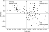 |
Fig. 9 Age-metallicity relation for our sample. |
Abundance correlations with metallicities and ages.
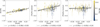 |
Fig. 10 Trends of [Eu/H], [Th/H], and [Th/Eu] against metallicity. The symbols are the same as in Fig. 4, with the color codes indicating age. The best-fit linear regression is given below each panel, and the shaded region indicates the confidence interval of the fit. We find significant trends for [Eu/H] and [Th/H], but not for [Th/Eu] (see text). |
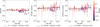 |
Fig. 11 Trends of [Eu/H], [Th/H], and [Th/Eu] against age in logarithmic scale. The symbols are the same as in Fig. 10, with color codes indicating metallicities. We find a significant trend for [Th/Eu], but not for [Eu/H] and [Th/H] (see text). |
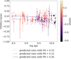 |
Fig. 12 Trend of [Th/Eu]now with age. The dashed lines indicate the predicted present-day ratio assuming a constant PR. The solar symbol marks the solar value, and the black stars indicate the two RPE stars, CS 31082-001 and HE 1523-0901. |
5.2 The implications on the r-process production
In this section, we discuss the interpretation of the correlations described above. First, we observe positive correlations for both Eu and Th with metallicities. The difference in slope of [Eu/H] - [Fe/H] and [Th/H]initial - [Fe/H] is 0.04 ± 0.10, showing that there is no significant difference in the strength of those correlations. This is further supported by the flat trend of [Th/Eu]initial against metallicity (see also Roederer et al. 2009). This finding aligns with standard galactic chemical evolution models, where the production of Eu and Th increases as the events that produce Fe also increase.
Second, we find a statistically significant positive correlation between [Th/Eu]initial and age. This may hint at a more efficient Th production in the early Universe, causing a slight increase in [Th/Eu]initial ratio toward older age. Such a scenario can be explained by different dominant r-process source(s) in the early and present-day Universe, i.e., short and long-timescale events. As the Universe evolves, the relative contributions of different sites of r-process events change, leading to the [Th/Eu]initial ratio’s dependency on age. There have been discussions supporting the combination of long and short-timescale r-process sources (e.g., Côté et al. 2019; Mishenina et al. 2022, and Farouqi et al. 2022). However, there is no clear consensus on short-timescale source(s) that can produce a high actinide-to-lanthanide ratio.
Even though CCSNe are commonly proposed as candidates for short timescale r-process sources, the physical conditions do not favor heavy r-process element production (Wanajo et al. 2011; Janka 2012; Goriely & Janka 2016). Instead, compact binary mergers such as NSMs or NS-BH mergers are more favored, as their ejecta are more neutron-rich, resulting in lanthanides and actinides production (Wanajo et al. 2014; Just et al. 2015). Rare types of CCSNe, such as MRD SNe, may produce actinides, but likely only in small quantities, indicating that this type of event contributes a minimal fraction of the universal r-process material (Reichert et al. 2023). However, the current models for CCSNe and NSMs still have limitations in their detailed treatment of the underlying physics (see, for example, Goriely & Janka 2016). Therefore, further investigation is necessary to develop a model that can produce actinides on a short timescale under realistic astrophysical conditions.
It is also crucial to contextualize our results within the universal [Th/Eu] ratios, including the more metal-poor regime not covered in our sample. Metal-poor stars exhibit a large scatter of >1.0 dex in [Th/Eu]now at [Fe/H] ≤ −1.8 (see, for example, Ren et al. (2012) and Fig. 5 of Wu et al. (2022). Since these stars are very metal-poor, it is reasonable to assume they have ages around 13 Gyr, which would lead to a similar amount of scatter in [Th/Eu]initial . The abundance scatter in metal-poor stars is commonly explained by the environmental factors of their birthplace. These stars typically reside in the galactic halo and smaller systems, where stochastic r-process events in the early Universe and inhomogeneous mixing of the natal cloud naturally result in a large star-to-star abundance scatter.
In Fig. 12, we present two examples of RPE halo stars, CS 31082-001 and HE 1523-0901, previously analyzed by Cayrel et al. (2001) and Frebel et al. (2007). Their ages are estimated by employing various chronometers, including U/Th, U/Ir, and U/Os, resulting in a median age of 12.5 Gyr for CS 31082-001 (Cayrel et al. 2001) and a weighted average of 13.2 Gyr for HE 1523-0901 (Frebel et al. 2007). The current [Th/Eu]now value for CS 31082-001 exceeds the predicted ratio from decay, even when assuming the highest PR, while the value for HE 1523-0901 falls between the highest and lowest PRs. Although this may support the variation of PR found in our study, it cannot be directly concluded for these stars due to the environmental factors mentioned above. On the other hand, in our sample of disk stars, a larger number of events and a more homogeneous chemical mixing are expected to contribute to the observed stellar abundances. Even though some degree of inhomogeneous mixing in the disk cannot be ruled out, especially in the case of old stars, the wide age distribution of our sample allows for a more robust analysis of PR variation. Therefore, our study shows that, while [Th/Eu]initial is correlated with age, environmental factors also play an important role in shaping the [Th/Eu] distribution.
5.3 Further improvements and prospects
The improved precision of the Th abundance will provide a more stringent constraint on the r-process evolution, especially the actinides, in the metal-rich regime. To obtain more accurate and reliable abundances, an improvement could be made to the measurements of the atomic properties of this line. As mentioned in Sect. 3, there is quite a large uncertainty, 10% of the gf value, in the Th line analyzed in this study. Improving the precision of the oscillator strength would minimize the systematic offset in the Th abundance measurement.
Another important point is compiling a complete line list including all the atomic and molecular lines in the region, especially the strong lines most likely to appear in the stellar spectra. This is especially crucial for lines that might be a source of blending in the Th line, as in the case of the CN 5989.054 Å line. The precision of the data for the other lines is also of importance, for example, the oscillator strengths of the neighboring Si I lines and the wavelength of the Nd II line. While these lines do not directly overlap with the Th line, the overall fitting accuracy would improve the local continuum placement.
Furthermore, as the uncertainties in the Th abundance measurement are dominated by the fitting uncertainty, increasing the S/N in the Th region helps reduce the measurement uncertainties. This is especially important in cases where the Th line feature is weak.
Analyzing a more homogeneous sample, such as globular clusters, would help better constrain the abundance trends with metallicities. As globular clusters consist of stars with similar ages, there would be no overlap between different populations of stars, minimizing the noise in analyzing the abundance trends. This would provide a constraint for old metal-poor stars around −2.5 ≤ [Fe/H] ≤ −0.5. The constraint for young metal-rich stars could be provided by studying open clusters in the metallicity range of −0.5 ≤ [Fe/H] ≤ 0.3. Combining both types of samples would then give a complete picture of the abundance trends with age, without overlapping the populations. Such studies are currently scarce due to the difficulty of detecting the Th line, with some examples being Sneden et al. (2000b) and Yong et al. (2008). However, the small sample sizes hinder any conclusion on the Th abundance trend.
The correlation of the [Th/Eu]initial ratio with stellar age indicates that the Th/Eu PR is not constant. This emphasizes the need to constrain its evolution through both observational data and theoretical calculations. Previous discussions of the varying PR can be found in works by Hill et al. (2017) and Ji & Frebel (2018), which demonstrate that in some cases, tuning the PR is necessary to derive a physical stellar age using the Th/Eu chronometer. This suggests that using the Th/Eu ratio as a chronometer should be done with caution. An alternative is the Th/U chronometer, which may offer reduced systematic uncertainties in the PR due to the close mass numbers of Th and U (Cowan et al. 1999; Schatz et al. 2002). However, this approach comes with the challenge of detecting U lines and accurately determining their abundance.
Our results suggest that Th is more efficiently produced in the early Universe, pointing to the necessity of actinide production in short-timescale source(s). Currently, there is insufficient evidence supporting any particular source. Although NSMs are preferred over CCSNe in terms of physical conditions, concerns about delay times remain. This study provides observational constraints for future research into theoretical models of actinide production in the early Universe.
6 Conclusions
We derived abundance measurements for Th and Eu for a sample of red giant stars with −0.7 < [Fe/H] < 0.4. We demonstrate that Th abundance can be derived from the Th II line at 5989 Å with higher precision by careful treatment of the atomic data and blending. While we find that the [Eu/Fe] abundance is well constrained, there is a wider spread on [Th/Fe]. For the first time, we derive the initial Th abundance using prior age information from seismology. While individual measurement uncertainty may be considerable, our large sample size enables us to examine statistically significant correlations between abundance ratios with metallicities and ages.
We identify the following key findings:
There is a significant correlation between [Eu/H] and [Fe/H], as well as between [Th/H]initial and [Fe/H], as expected from standard galactic chemical evolution models.
On the other hand, there is no significant trend between [Th/Eu]initial and [Fe/H], suggesting that [Th/Eu] remains broadly uniform across metallicities covered in our sample.
The abundance ratio [Th/Eu]initial shows a significant correlation with age, which may point to different contributions of the dominant r-process site in the early Universe compared to the present day.
Our analysis can be improved by minimizing the uncertainties in Th abundance, for example, by increasing the precision of the line data, completing the line list, and increasing the spectral S /N. More accurate measurements of Th abundance would benefit the understanding of actinide evolution in metal-rich stars.
Acknowledgements
This research is based on data collected at Subaru Telescope, which is operated by the National Astronomical Observatory of Japan. We are honored and grateful for the opportunity to observe the Universe from Mau-nakea, which has cultural, historical, and natural significance in Hawaii. The data are retrieved from the JVO portal (http://jvo.nao.ac.jp/portal) operated by NAOJ. This work was supported in part by JSPS KAKENHI Grant Numbers JP21H04499 and JP20H05855, and by a Spinoza grant awarded to Amina Helmi. T.M. acknowledges support from a Gliese Fellowship at the Zentrum für Astronomie, University of Heidelberg. A.A. is grateful to Nicholas Storm for helpful discussions regarding the use of TSFitPy.
Appendix A Additional tables
Abundance results, stellar parameters, seismic masses, and ages for Arcturus and our main sample
Line list for the Th 5989 Å region
CN lines responsible for and used to constrain contamination of Th and Eu features
References
- Alvarez, R., & Plez, B. 1998, A&A, 330, 1109 [NASA ADS] [Google Scholar]
- Aoki, W., Honda, S., Sadakane, K., & Arimoto, N. 2007, PASJ, 59, L15 [NASA ADS] [Google Scholar]
- Arnould, M., Goriely, S., & Takahashi, K. 2007, Phys. Rep., 450, 97 [Google Scholar]
- Asplund, M., Grevesse, N., Sauval, A. J., & Scott, P. 2009, ARA&A, 47, 481 [NASA ADS] [CrossRef] [Google Scholar]
- Bisterzo, S., Travaglio, C., Gallino, R., Wiescher, M., & Käppeler, F. 2014, ApJ, 787, 10 [NASA ADS] [CrossRef] [Google Scholar]
- Botelho, R. B., Milone, A. d. C., Meléndez, J., et al. 2019, MNRAS, 482, 1690 [NASA ADS] [CrossRef] [Google Scholar]
- Brooke, J. S. A., Ram, R. S., Western, C. M., et al. 2014, ApJS, 210, 23 [NASA ADS] [CrossRef] [Google Scholar]
- Burbidge, E. M., Burbidge, G. R., Fowler, W. A., & Hoyle, F. 1957, Rev. Mod. Phys., 29, 547 [NASA ADS] [CrossRef] [Google Scholar]
- Cameron, A. G. W. 1957, AJ, 62, 9 [CrossRef] [Google Scholar]
- Cayrel, R., Hill, V., Beers, T. C., et al. 2001, Nature, 409, 691 [CrossRef] [PubMed] [Google Scholar]
- Cescutti, G., & Chiappini, C. 2014, A&A, 565, A51 [NASA ADS] [CrossRef] [EDP Sciences] [Google Scholar]
- Corliss, C. H. 1979, MNRAS, 189, 607 [Google Scholar]
- Côté, B., Eichler, M., Arcones, A., et al. 2019, ApJ, 875, 106 [Google Scholar]
- Cowan, J. J., McWilliam, A., Sneden, C., & Burris, D. L. 1997, ApJ, 480, 246 [Google Scholar]
- Cowan, J. J., Pfeiffer, B., Kratz, K. L., et al. 1999, ApJ, 521, 194 [NASA ADS] [CrossRef] [Google Scholar]
- Cowan, J. J., Sneden, C., Lawler, J. E., et al. 2021, Rev. Mod. Phys., 93, 015002 [Google Scholar]
- del Peloso, E. F., da Silva, L., Porto de Mello, G. F., & Arany-Prado, L. I. 2005, A&A, 440, 1153 [NASA ADS] [CrossRef] [EDP Sciences] [Google Scholar]
- Domoto, N., Tanaka, M., Wanajo, S., & Kawaguchi, K. 2021, ApJ, 913, 26 [NASA ADS] [CrossRef] [Google Scholar]
- Domoto, N., Wanajo, S., Tanaka, M., Kato, D., & Hotokezaka, K. 2025, ApJ, 978, 99 [Google Scholar]
- Farouqi, K., Thielemann, F. K., Rosswog, S., & Kratz, K. L. 2022, A&A, 663, A70 [NASA ADS] [CrossRef] [EDP Sciences] [Google Scholar]
- Frebel, A., Christlieb, N., Norris, J. E., et al. 2007, ApJ, 660, L117 [NASA ADS] [CrossRef] [Google Scholar]
- Gerber, J. M., Magg, E., Plez, B., et al. 2023, A&A, 669, A43 [NASA ADS] [CrossRef] [EDP Sciences] [Google Scholar]
- Gopka, V. F., Yushchenko, A. V., Shavrina, A. V., & Perekhod, A. V. 1999, Kinematika i Fizika Nebesnykh Tel, 15, 447 [Google Scholar]
- Gopka, V. F., Vasil’Eva, S. V., Yushchenko, A. V., & Andrievsky, S. M. 2007, Odessa Astron. Pub., 20, 58 [Google Scholar]
- Goriely, S., & Arnould, M. 2001, A&A, 379, 1113 [NASA ADS] [CrossRef] [EDP Sciences] [Google Scholar]
- Goriely, S., & Janka, H. T. 2016, MNRAS, 459, 4174 [Google Scholar]
- Guiglion, G., de Laverny, P., Recio-Blanco, A., & Prantzos, N. 2018, A&A, 619, A143 [NASA ADS] [CrossRef] [EDP Sciences] [Google Scholar]
- Guo, Y., Storm, N., Bergemann, M., et al. 2025, A&A, 693, A211 [NASA ADS] [CrossRef] [EDP Sciences] [Google Scholar]
- Gustafsson, B., Edvardsson, B., Eriksson, K., et al. 2008, A&A, 486, 951 [NASA ADS] [CrossRef] [EDP Sciences] [Google Scholar]
- Heiter, U., Lind, K., Bergemann, M., et al. 2021, A&A, 645, A106 [EDP Sciences] [Google Scholar]
- Hill, V., Plez, B., Cayrel, R., et al. 2002, A&A, 387, 560 [CrossRef] [EDP Sciences] [Google Scholar]
- Hill, V., Christlieb, N., Beers, T. C., et al. 2017, A&A, 607, A91 [NASA ADS] [CrossRef] [EDP Sciences] [Google Scholar]
- Holmbeck, E. M., Frebel, A., McLaughlin, G. C., et al. 2019, ApJ, 881, 5 [NASA ADS] [CrossRef] [Google Scholar]
- Holmbeck, E. M., Barnes, J., Lund, K. A., et al. 2023, ApJ, 951, L13 [Google Scholar]
- Holweger, H. 1980, The Observatory, 100, 155 [NASA ADS] [Google Scholar]
- Honda, S., Aoki, W., Kajino, T., et al. 2004, ApJ, 607, 474 [NASA ADS] [CrossRef] [Google Scholar]
- Honda, S., Aoki, W., Ishimaru, Y., Wanajo, S., & Ryan, S. G. 2006, ApJ, 643, 1180 [NASA ADS] [CrossRef] [Google Scholar]
- Ivans, I. I., Simmerer, J., Sneden, C., et al. 2006, ApJ, 645, 613 [NASA ADS] [CrossRef] [Google Scholar]
- Janka, H.-T. 2012, Ann. Rev. Nucl. Part. Sci., 62, 407 [Google Scholar]
- Ji, A. P., & Frebel, A. 2018, ApJ, 856, 138 [NASA ADS] [CrossRef] [Google Scholar]
- Just, O., Bauswein, A., Ardevol Pulpillo, R., Goriely, S., & Janka, H. T. 2015, MNRAS, 448, 541 [NASA ADS] [CrossRef] [Google Scholar]
- Kajino, T., Aoki, W., Balantekin, A. B., et al. 2019, Prog. Part. Nucl. Phys., 107, 109 [NASA ADS] [CrossRef] [Google Scholar]
- Kasliwal, M. M., Kasen, D., Lau, R. M., et al. 2022, MNRAS, 510, L7 [Google Scholar]
- Kobayashi, C., Karakas, A. I., & Lugaro, M. 2020, ApJ, 900, 179 [Google Scholar]
- Koch, D. G., Borucki, W. J., Basri, G., et al. 2010, ApJ, 713, L79 [Google Scholar]
- Kratz, K.-L., Bitouzet, J.-P., Thielemann, F.-K., Moeller, P., & Pfeiffer, B. 1993, ApJ, 403, 216 [NASA ADS] [CrossRef] [Google Scholar]
- Kratz, K.-L., Farouqi, K., Pfeiffer, B., et al. 2007, ApJ, 662, 39 [NASA ADS] [CrossRef] [Google Scholar]
- Kurucz, R. 1993, ATLAS9 Stellar Atmosphere Programs and 2 km/s grid. Kurucz CD-ROM No. 13. Cambridge, 13 [Google Scholar]
- Liu, Y. J., Wang, L., Takeda, Y., Bharat Kumar, Y., & Zhao, G. 2019, MNRAS, 482, 4155 [Google Scholar]
- Magg, E., Bergemann, M., Serenelli, A., et al. 2022, A&A, 661, A140 [NASA ADS] [CrossRef] [EDP Sciences] [Google Scholar]
- Mashonkina, L., Ryabtsev, A., & Frebel, A. 2012, A&A, 540, A98 [NASA ADS] [CrossRef] [EDP Sciences] [Google Scholar]
- Mishenina, T. V., Pignatari, M., Korotin, S. A., et al. 2013, A&A, 552, A128 [NASA ADS] [CrossRef] [EDP Sciences] [Google Scholar]
- Mishenina, T., Pignatari, M., Gorbaneva, T., et al. 2022, MNRAS, 516, 3786 [NASA ADS] [CrossRef] [Google Scholar]
- Molero, M., Magrini, L., Matteucci, F., et al. 2023, MNRAS, 523, 2974 [NASA ADS] [CrossRef] [Google Scholar]
- Mosser, B., Goupil, M. J., Belkacem, K., et al. 2012, A&A, 540, A143 [NASA ADS] [CrossRef] [EDP Sciences] [Google Scholar]
- Naidu, R. P., Ji, A. P., Conroy, C., et al. 2022, ApJ, 926, L36 [CrossRef] [Google Scholar]
- Nilsson, H., Zhang, Z. G., Lundberg, H., Johansson, S., & Nordström, B. 2002, A&A, 382, 368 [NASA ADS] [CrossRef] [EDP Sciences] [Google Scholar]
- Nishimura, N., Sawai, H., Takiwaki, T., Yamada, S., & Thielemann, F. K. 2017, ApJ, 836, L21 [CrossRef] [Google Scholar]
- Noguchi, K., Aoki, W., Kawanomoto, S., et al. 2002, PASJ, 54, 855 [NASA ADS] [CrossRef] [Google Scholar]
- Pinsonneault, M. H., Zinn, J. C., Tayar, J., et al. 2025, ApJS, 276, 69 [NASA ADS] [CrossRef] [Google Scholar]
- Placco, V. M., Holmbeck, E. M., Frebel, A., et al. 2017, ApJ, 844, 18 [NASA ADS] [CrossRef] [Google Scholar]
- Placco, V. M., Almeida-Fernandes, F., Holmbeck, E. M., et al. 2023, ApJ, 959, 60 [NASA ADS] [CrossRef] [Google Scholar]
- Plez, B. 2012, Astrophysics Source Code Library [record ascl:1205.004] [Google Scholar]
- Radice, D., Perego, A., Hotokezaka, K., et al. 2018, ApJ, 869, 130 [Google Scholar]
- Ramírez, I., & Allende Prieto, C. 2011, ApJ, 743, 135 [Google Scholar]
- Reichert, M., Hansen, C. J., & Arcones, A. 2021, ApJ, 912, 157 [NASA ADS] [CrossRef] [Google Scholar]
- Reichert, M., Obergaulinger, M., Aloy, M. Á., et al. 2023, MNRAS, 518, 1557 [Google Scholar]
- Ren, J., Christlieb, N., & Zhao, G. 2012, A&A, 537, A118 [NASA ADS] [CrossRef] [EDP Sciences] [Google Scholar]
- Roederer, I. U., Kratz, K.-L., Frebel, A., et al. 2009, ApJ, 698, 1963 [NASA ADS] [CrossRef] [Google Scholar]
- Ryabchikova, T., Piskunov, N., Kurucz, R. L., et al. 2015, Phys. Scr, 90, 054005 [Google Scholar]
- Ryde, N., Edvardsson, B., Gustafsson, B., et al. 2009, A&A, 496, 701 [NASA ADS] [CrossRef] [EDP Sciences] [Google Scholar]
- Schatz, H., Toenjes, R., Pfeiffer, B., et al. 2002, ApJ, 579, 626 [NASA ADS] [CrossRef] [Google Scholar]
- Seeger, P. A., Fowler, W. A., & Clayton, D. D. 1965, ApJS, 11, 121 [NASA ADS] [CrossRef] [Google Scholar]
- Shah, S. P., Ezzeddine, R., Ji, A. P., et al. 2023, ApJ, 948, 122 [Google Scholar]
- Siegel, D. M. 2022, Nat. Rev. Phys., 4, 306 [NASA ADS] [CrossRef] [Google Scholar]
- Skúladóttir, Á., & Salvadori, S. 2020, A&A, 634, L2 [NASA ADS] [CrossRef] [EDP Sciences] [Google Scholar]
- Sneden, C., Cowan, J. J., Ivans, I. I., et al. 2000a, ApJ, 533, L139 [NASA ADS] [CrossRef] [Google Scholar]
- Sneden, C., Johnson, J., Kraft, R. P., et al. 2000b, ApJ, 536, L85 [NASA ADS] [CrossRef] [Google Scholar]
- Sneden, C., Lucatello, S., Ram, R. S., Brooke, J. S. A., & Bernath, P. 2014, ApJS, 214, 26 [Google Scholar]
- Sneden, C., McWilliam, A., Preston, G. W., et al. 1996, ApJ, 467, 819 [NASA ADS] [CrossRef] [Google Scholar]
- Storm, N., & Bergemann, M. 2023, MNRAS, 525, 3718 [NASA ADS] [CrossRef] [Google Scholar]
- Strassmeier, K. G., Ilyin, I., & Weber, M. 2018, A&A, 612, A45 [NASA ADS] [CrossRef] [EDP Sciences] [Google Scholar]
- Surman, R., McLaughlin, G. C., Ruffert, M., Janka, H. T., & Hix, W. R. 2008, ApJ, 679, L117 [NASA ADS] [CrossRef] [Google Scholar]
- Takeda, Y., & Tajitsu, A. 2015, MNRAS, 450, 397 [Google Scholar]
- Takeda, Y., Sato, B., Kambe, E., Sadakane, K., & Ohkubo, M. 2002, PASJ, 54, 1041 [NASA ADS] [Google Scholar]
- Takeda, Y., Ohkubo, M., Sato, B., Kambe, E., & Sadakane, K. 2005, PASJ, 57, 27 [NASA ADS] [CrossRef] [Google Scholar]
- Takeda, Y., Sato, B., & Murata, D. 2008, PASJ, 60, 781 [NASA ADS] [CrossRef] [Google Scholar]
- Takeda, Y., Tajitsu, A., Sato, B., et al. 2016, MNRAS, 457, 4454 [Google Scholar]
- Tautvaišiene, G., Viscasillas Vázquez, C., Mikolaitis, Š., et al. 2021, A&A, 649, A126 [NASA ADS] [CrossRef] [EDP Sciences] [Google Scholar]
- Truran, J. W. 1981, A&A, 97, 391 [NASA ADS] [Google Scholar]
- Tsujimoto, T. 2021, ApJ, 920, L32 [Google Scholar]
- Van der Swaelmen, M., Hill, V., Primas, F., & Cole, A. A. 2013, A&A, 560, A44 [NASA ADS] [CrossRef] [EDP Sciences] [Google Scholar]
- Wanajo, S., Janka, H.-T., & Müller, B. 2011, ApJ, 726, L15 [NASA ADS] [CrossRef] [Google Scholar]
- Wanajo, S., Sekiguchi, Y., Nishimura, N., et al. 2014, ApJ, 789, L39 [Google Scholar]
- Wanajo, S., Fujibayashi, S., Hayashi, K., et al. 2024, Phys. Rev. Lett., 133, 241201 [Google Scholar]
- Warfield, J. T., Zinn, J. C., Schonhut-Stasik, J., et al. 2024, AJ, 167, 208 [NASA ADS] [CrossRef] [Google Scholar]
- Watson, D., Hansen, C. J., Selsing, J., et al. 2019, Nature, 574, 497 [NASA ADS] [CrossRef] [Google Scholar]
- Wehmeyer, B., Pignatari, M., & Thielemann, F. K. 2015, MNRAS, 452, 1970 [NASA ADS] [CrossRef] [Google Scholar]
- Wehmeyer, B., Fröhlich, C., Côté, B., Pignatari, M., & Thielemann, F. K. 2019, MNRAS, 487, 1745 [NASA ADS] [CrossRef] [Google Scholar]
- Westin, J., Sneden, C., Gustafsson, B., & Cowan, J. J. 2000, ApJ, 530, 783 [NASA ADS] [CrossRef] [Google Scholar]
- Winteler, C., Käppeli, R., Perego, A., et al. 2012, ApJ, 750, L22 [Google Scholar]
- Worley, C. C., Cottrell, P. L., Freeman, K. C., & Wylie-de Boer, E. C. 2009, MNRAS, 400, 1039 [NASA ADS] [CrossRef] [Google Scholar]
- Wu, Z., Ricigliano, G., Kashyap, R., Perego, A., & Radice, D. 2022, MNRAS, 512, 328 [Google Scholar]
- Xie, X.-J., Shi, J., Yan, H.-L., et al. 2024, ApJ, 970, L30 [NASA ADS] [CrossRef] [Google Scholar]
- Yong, D., Karakas, A. I., Lambert, D. L., Chieffi, A., & Limongi, M. 2008, ApJ, 689, 1031 [NASA ADS] [CrossRef] [Google Scholar]
- Yu, J., Huber, D., Bedding, T. R., et al. 2018, ApJS, 236, 42 [NASA ADS] [CrossRef] [Google Scholar]
R. L. Kurucz online database of molecular line lists, accessible at http://kurucz.harvard.edu/molecules/cn/cnaxbrookek.asc
All Tables
Abundance results, stellar parameters, seismic masses, and ages for Arcturus and our main sample
CN lines responsible for and used to constrain contamination of Th and Eu features
All Figures
|
Fig. 1 Top panel: our fitting result of the Eu line for Arcturus. The dotted black line shows the observed spectrum; the solid red line shows the best-fit spectrum; and the dashed gray line shows the spectrum without Eu contribution. Bottom panel: our fitting result of the Th line in Arcturus. The dashed blue lines show the synthetic spectrum before the adjustment of the line list; the solid red line shows the final fitting result; and the dashed gray line shows the synthetic spectrum without Th contribution. |
| In the text | |
|
Fig. 2 CN line used to constrain the strength of CN absorption. The solid blue line indicates the synthetic spectrum assuming [C/Fe] and [N/Fe] from Ryde et al. (2009), while the solid red line indicates our best-fit result (see Sect. 3.2). The dashed gray line indicates the synthetic spectrum without CN contribution. |
| In the text | |
|
Fig. 3 Our estimate of the CN line strength (equivalent widths) derived by fixing the C abundance and varying N abundance. The strength of the CN line varies in the region of the Th and Eu lines, as indicated by the EW of the CN lines at 5972.985 and 6644.3 À. |
| In the text | |
|
Fig. 4 From left to right: trend of [Eu/Fe], [Th/Fe], and [Th/Eu] against metallicities, respectively. The blue-filled circles show the results of Mishenina et al. (2022), and the red-filled circles show our results. The open red circles show the outliers discussed in the text, and the downward arrows denote upper limits. The yellow pentagon denotes Arcturus. |
| In the text | |
|
Fig. 5 Observed spectra of the Th line region (dots) compared to synthetic ones (lines). The fitting results of four stars in our sample with different metallicities show varying strengths of the CN line contribution. The solid red line shows the best-fit spectrum, and the dashed gray line shows the synthetic spectrum without Th contribution (i.e., the contribution from the CN line). The second left panel shows the case of the star with a high Th abundance, KIC4243623. |
| In the text | |
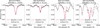 |
Fig. 6 Same as in Fig. 5, but for the Eu line region. |
| In the text | |
|
Fig. 7 Difference between [Eu/Fe] in Liu et al. (2019) and this study (Δ[Eu/Fe] = [Eu/Fe]literature - [Eu/Fe]this work). |
| In the text | |
|
Fig. 8 [Th/Fe] distribution of the stars in our sample, color-coded according to metallicities. There is no correlation between the Th abundance and Teff or [Fe/H], supporting that our measurement is not affected by systematics in stellar parameters. |
| In the text | |
|
Fig. 9 Age-metallicity relation for our sample. |
| In the text | |
|
Fig. 10 Trends of [Eu/H], [Th/H], and [Th/Eu] against metallicity. The symbols are the same as in Fig. 4, with the color codes indicating age. The best-fit linear regression is given below each panel, and the shaded region indicates the confidence interval of the fit. We find significant trends for [Eu/H] and [Th/H], but not for [Th/Eu] (see text). |
| In the text | |
|
Fig. 11 Trends of [Eu/H], [Th/H], and [Th/Eu] against age in logarithmic scale. The symbols are the same as in Fig. 10, with color codes indicating metallicities. We find a significant trend for [Th/Eu], but not for [Eu/H] and [Th/H] (see text). |
| In the text | |
|
Fig. 12 Trend of [Th/Eu]now with age. The dashed lines indicate the predicted present-day ratio assuming a constant PR. The solar symbol marks the solar value, and the black stars indicate the two RPE stars, CS 31082-001 and HE 1523-0901. |
| In the text | |
Current usage metrics show cumulative count of Article Views (full-text article views including HTML views, PDF and ePub downloads, according to the available data) and Abstracts Views on Vision4Press platform.
Data correspond to usage on the plateform after 2015. The current usage metrics is available 48-96 hours after online publication and is updated daily on week days.
Initial download of the metrics may take a while.