| Issue |
A&A
Volume 699, July 2025
|
|
|---|---|---|
| Article Number | A87 | |
| Number of page(s) | 12 | |
| Section | The Sun and the Heliosphere | |
| DOI | https://doi.org/10.1051/0004-6361/202554580 | |
| Published online | 02 July 2025 | |
Magnetic flux cancellation in a flux-emergence magnetohydrodynamics simulation of coronal hole eruptions and jets
Physics Department, University of Ioannina, Ioannina GR-45110, Greece
⋆ Corresponding author: spatsour@uoi.gr
Received:
17
March
2025
Accepted:
8
May
2025
Context. Observations have demonstrated that magnetic flux cancellation can be associated with coronal jets and eruptions taking place in coronal holes. However, magnetic flux cancellation is barely reported in magnetohydrodynamics (MHD) simulations of coronal jets and eruptions which employ emerging twisted flux tubes.
Aims. We search for signatures of magnetic flux cancellation in a 3D resistive MHD flux-emergence simulation of coronal jets and eruptions in a coronal-hole-like environment.
Methods. To do this, we analysed the output from a 3D MHD simulation of an emerging twisted horizontal flux tube from the convection zone into the solar atmosphere. The simulation considered the impact of neutral hydrogen on the magnetic induction equation, that is, it employed partially ionised plasma. Standard and blowout jets as well as eruptions were observed during the simulation.
Results. We observe clear evidence of magnetic flux cancellation in a short segment along the internal polarity-inversion line (iPIL) of the photospheric Bz during an extended period of the simulation characterised by eruptions and blowout jets. Converging magnetic footpoint motions at ≈1 km s−1 carried sheared fields within the magnetic tails of the emerging flux tube towards the iPIL. These fields reconnect at the iPIL and generate concave-upward and slowly rising field lines causing a flux decrease that is associated with magnetic flux cancellation. The magnetic flux decreases at a rate of ≈3.2×10¹⁸ Mx hour−1 and about 15–20% during intervals of individual eruptions and jets.
Conclusions. We show evidence of magnetic flux cancellation in 3D MHD simulations of coronal hole eruptions and jets associated with an emerging twisted flux tube. The magnetic flux cancellation can be traced up to about 520 km above the photosphere and might contribute to the formation of pre-eruptive magnetic flux rope seeds. Although our results are consistent with several basic aspects of magnetic flux-cancellation observations associated with coronal jets, the observations nevertheless also suggest that cancellation involves much larger fractions of the available flux than our numerical simulation. We supply avenues to address this discrepancy in future work.
Key words: Sun: activity / Sun: atmosphere / Sun: corona
© The Authors 2025
 Open Access article, published by EDP Sciences, under the terms of the Creative Commons Attribution License (https://creativecommons.org/licenses/by/4.0), which permits unrestricted use, distribution, and reproduction in any medium, provided the original work is properly cited.
This article is published in open access under the Subscribe to Open model. Subscribe to A&A to support open access publication.
1. Introduction
Coronal jets are narrow transient collimated outflows that are observed all over the Sun: in the quiet Sun (QS), in coronal holes (polar and equatorial), and in active regions (e.g. see the reviews Raouafi et al. 2016; Shen 2021; Schmieder 2022). They are mainly observed in the soft X-rays (SXRs) and in the extreme ultraviolet (EUV) with imagers and spectrometers and in the white light with coronagraphs. It is important to build a concrete understanding of the physical mechanisms that form and evolve coronal jets and small-scale eruptions in general because these phenomena might represent an important contributor to the solar wind mass supply (e.g. Raouafi et al. 2023; Chitta et al. 2023). In addition, given the relative simplicity of the magnetic configurations involved in coronal jets, studying them and eventually understanding them may also provide important clues about large-scale eruptive solar phenomena (e.g. Sterling et al. 2015; Wyper et al. 2017; Kumar et al. 2021). Significant changes in the magnetic helicity and free magnetic energy, similarly to what is observed during larger-scale eruptive phenomena, are recorded during coronal jets, as suggested by observations and Magnetohydrodynamics (MHD) modelling (e.g. Nindos et al. 2024; Moraitis et al. 2024). The multitude of wavelength bands and instruments used in observations of coronal jets and related phenomena gives rise to a plethora of various descriptive terms and classifications.
A proposed classification of coronal jets is in terms of “standard” and “blowout” jets Moore et al. (2010). A standard jet occurs when reconnection between an emerging magnetic bipole and the ambient large-scale open magnetic field takes place (e.g. Yokoyama & Shibata 1996; Moreno-Insertis et al. 2008; Archontis & Hood 2013; Moreno-Insertis & Galsgaard 2013; Fang et al. 2014). Blowout jets occur when stressed and occasionally twisted core magnetic fields first erupt and then reconnect with the ambient large-scale open magnetic field (e.g. Pariat et al. 2009; Archontis & Hood 2013). Therefore, a key characteristic of blowout jets is that a small-scale eruption is in order, and leads to the opening of previously closed sheared or twisted core fields that are channelled into the resulting blowout jets.
Magnetic flux cancellation is a frequently observed phenomenon in the photosphere of the QS, coronal holes, and active regions. It occurs when patches of vertical photospheric magnetic fields of opposite polarity with a similar magnetic field magnitude approach each other and their magnetic flux decreases (Livi et al. 1985; Martin et al. 1985; Martin 1988). Frequently, periods of magnetic flux cancellation occur in tandem with multi-scale eruptive activity that ranges all way from proper coronal mass ejections (CMEs) down to coronal jets and transient outflows (e.g. Green & Kliem 2009; Savcheva et al. 2012; Yardley et al. 2018; Panesar et al. 2018; Chintzoglou et al. 2019; Moore et al. 2022). In addition to being considered a potential trigger mechanism for eruptive phenomena and transient outflows and a supplier of solar wind mass and coronal heating (e.g. Pontin et al. 2024), magnetic flux cancellation is also a viable formation mechanism of pre-eruptive magnetic flux ropes (MFRs; e.g. van Ballegooijen & Martens 1989; Amari et al. 2003; Mackay & van Ballegooijen 2006; Aulanier et al. 2010; Hassanin et al. 2022; Xing et al. 2024). MFRs are coherent arrangements of twisted magnetic fields that coil around a common axis (e.g. see the definitions and pertinent discussions in Patsourakos et al. 2020), and they are a candidate pre-eruptive magnetic configuration.
There exist three possibilities to deal with the decrease in the magnetic flux that is associated with magnetic flux cancellation: i) emergence of U-loops; ii) submergence of Ω-loops, and iii) magnetic reconnection at or close to the photosphere that creates pairs of U- and Ω-loops (for a schematic of these three cases, we refer to Fig. 2 in Zwaan 1987). The third scenario generates both U- and Ω-loops that emerge and submerge, respectively. It then depends on whether the height at which the reconnection occurs is somewhat below or above the height at which magnetic field information is available, so that magnetic flux cancellation is detected via emerging U- or submerging Ω-loops, respectively. Observations of magnetic flux cancellation give rise to cases consistent with either emerging U-loops (e.g. van Driel-Gesztelyi et al. 2000; Bernasconi et al. 2002; Bellot Rubio & Beck 2005) or submerging Ω-loops (e.g. Harvey et al. 1999; Chae et al. 2004; Yang et al. 2009; Takizawa et al. 2012).
Observations by the Atmospheric Imaging Assembly (AIA) and Helioseismic and Magnetic Imager (HMI) on board the Solar Dynamics Observatory (SDO) showed varying proportions of coronal jets and small-scale eruptions associated with magnetic flux cancellation. McGlasson et al. (2017) analysed 30 equatorial coronal hole (ECH) and 30 QS jets and found that 85% of them were associated with magnetic flux cancellation. Mou et al. (2018) studied 21 small-scale eruptions stemming from 11 QS coronal bright points (CBPs) and found that 19 of these eruptions were associated with magnetic flux cancellation. Panesar et al. (2018) showed that magnetic flux cancellation was associated with 13 ECH jets containing mini-filament material. Moore et al. (2022) analysed 43 microflares in ECHs that were associated with small-scale bipolar ephemeral active regions with a typical span of 10 Mm. 18 of the microflares were associated with blowout jets, and magnetic flux cancellation before and during those jets was reported. Recent Solar Orbiter Extreme-Ultraviolet Imager (EUI) ultra-high spatial resolution observations of five small-scale coronal jets showed that three of them were associated with magnetic flux cancellation (Panesar et al. 2023). These studies also suggest that magnetic flux cancellation might be the trigger of the reported eruptions and jets. On the other hand, Kumar et al. (2019) analysed 27 ECH jets and found that only 6 of them were associated with magnetic flux cancellation that occurred before or during them. Muglach (2021) applied local correlation tracking to white-light photospheric images at the feet of a sample of 35 ECH jets and found evidence of converging motions and magnetic flux cancellation in four cases, and eight more complex cases, featuring both flux emergence and magnetic flux cancellation. Finally, recent joint EUI-HMI observations of 627 small-scale QS brightenings that occurred above concentrations of strong bipolar magnetic fields showed that only about 8% of these events were associated with magnetic flux cancellation (Nelson et al. 2024). The smallest magnetic flux emergence or cancellation events might be missed by the HMI resolution, as was noted for example by Nóbrega-Siverio et al. (2024), Georgoulis et al. (2025). A recent spectroscopic study of two jets in an ECH showed no evidence of magnetic flux cancellation in HMI observations (Koletti et al. 2024).
The MHD modelling of coronal jets and of eruptive solar phenomena in the low solar atmosphere in general may be cast into two broad categories: surface-driven and flux-emergence models (e.g. consult the recent reviews of Chen 2011; Raouafi et al. 2016; Green et al. 2018; Archontis & Syntelis 2019; Patsourakos et al. 2020; Shen 2021; Schmieder 2022). Surface-driven models employ simulation boxes that only incorporate the solar atmosphere, and they therefore span the photosphere, chromosphere, the transition region, and a segment of the lower corona. These models are driven by prescribed photospheric flow fields. Flux-emergence models typically include a part of the upper convection zone along with a segment covering the stratified atmosphere above it. These models are driven by the emergence of buoyant horizontal or toroidal twisted flux tubes from the convection zone into the solar atmosphere. In addition to prescribing the specifics (e.g. distribution of twist and a density deficit) of the sub-photospheric flux tubes, the subsequent evolution of the system including emergence, build-up of magnetic energy, shear and twist and eruptive activity is rather self-consistent.
Magnetic flux cancellation in surface-driven models and simulations was addressed by various authors (e.g. van Ballegooijen & Martens 1989; Amari et al. 2003; Mackay & van Ballegooijen 2006; Aulanier et al. 2010; Syntelis et al. 2019; Færder et al. 2023; Pontin et al. 2024). In order to achieve magnetic flux cancellation, these models and simulations typically involved a combination of postulated converging and shearing photospheric flow fields along with magnetic diffusion of the normal component of the magnetic field via prescribed tangential electric fields. Imposing appropriate sub-photospheric velocity fields was also shown to give rise to magnetic flux cancellation (Rempel et al. 2023).
Magnetic flux cancellation in flux-emergence simulations was discussed in detail by Magara (2011) and Fang et al. (2012). Both studies involved the emergence of a horizontal twisted flux tube from the convection zone into the solar atmosphere. Magara (2011) reported that magnetic flux cancellation was caused by the emergence and subsequent convergence of U-loops in the related polarity-inversion line (PIL) of the photospheric Bz, where Bz changes sign when the PIL is crossed. The U-loops might emerge against the gravity of the plasma collected in their concave upward segments, that is, magnetic dips, if they are shallow enough so that mass can drain. This essentially facilitates the rise of the U-loop. However, deep U-loops are not able not rise, and their legs would therefore be pinched off and reconnect. In both cases, signatures of magnetic flux cancellation are expected.
Fang et al. (2012) reported that photospheric convective and shearing motions carried emerging magnetic fields of opposite polarity in the PIL where they reconnected in a tether-cutting fashion (e.g. Moore et al. 2001). The reconnection gave rise to magnetic flux cancellation signatures, and an MFR formed. None of these simulations reported eruptive activity. To the best to our knowledge, the studies by Magara (2011) and Fang et al. (2012) are the only 3D MHD simulations of emerging twisted flux tubes that reported a magnetic flux cancellation.
Nóbrega-Siverio & Moreno-Insertis (2022) discussed 2D Bifrost flux-emergence simulations in a magnetic-null configuration within a coronal hole and studied the formation and dynamics of a CBP in terms of microflares, eruptions, and jets. In this simulation, flux emergence is related to convection-mediated dynamics. The authors noted that the photospheric magnetic flux at the feet of the CBP decreased for a time, which they attributed to magnetic flux cancellation. Panesar et al. (2023) reported Bifrost simulations of the injection of a horizontal flux sheet with a temporally varying strength from the convection zone into the solar atmosphere. They analysed five small-scale jets in detail and found that four of them were triggered by magnetic flux cancellation. The reported jets contained cool plasma. The simulations by Nóbrega-Siverio & Moreno-Insertis (2022) and Panesar et al. (2023) did not employ emerging twisted flux tubes.
We therefore conclude that there is a lack of detailed investigations of magnetic flux cancellation in MHD simulations of emerging twisted flux tubes that lead to coronal jets and eruptions in coronal holes. This is the focus of our study and a timely investigation, also in view of jet observations showing evidence of magnetic flux cancellation. In Section 2 we briefly describe our simulation, Section 3 presents the overall behaviour of our simulation, Section 4 discusses the characteristics and origins of the detected magnetic flux cancellation in detail and describes its implications for pre-eruptive MFRs, and Section 5 finally contains a summary and a discussion of our results. It also supplies comparisons of our simulation results with pertinent observations and MHD models.
2. Simulation
We employed output from a flux-emergence simulation using the code Lare3D (Arber et al. 2001), which solves the single-fluid ressistive MHD equations in 3D. The simulation, reported by Chouliaras & Archontis (in prep.), employed partial ionisation of the hydrogen in the magnetic induction equation. For more details on the implementation and the overall impact of partial ionisation of hydrogen in flux emergence in 3D MHD simulations, we refer to Chouliaras et al. (2023) and Chouliaras & Archontis (2025). The same simulation was also recently analysed by Moraitis et al. (2024), who studied the free magnetic energy and magnetic helicity evolution in the simulation box and its relation to coronal jets and eruptions. The simulation box was a 4203 voxel cube. The sides of each voxel were 180 km long, and therefore, the simulation box spanned about 65 Mm in each dimension. The simulation box included an ≈7 Mm thick upper convection zone layer at its bottom, and photospheric, chromospheric, transition region, and coronal layers were also included. The photospheric layer corresponds to the xy plane of the simulation box at an appropriate height. A cylindrical and uniformly twisted flux tube was placed 2.3 Mm below the photosphere with its axis running along the y-axis of the simulation box. Given an ascribed density deficit along a segment of the flux tube, the tube becomes buoyant and eventually emerges into a background isothermal atmosphere. The background atmosphere is permeated with an almost vertical magnetic field that forms an angle of ≈11 degrees with the vertical and uniform positive-polarity ambient magnetic field having a magnitude of ≈10 Gauss. In this way, our simulation emulated the emergence of a bipolar region within a coronal hole-like environment. The results from the simulation were damped in 86.9 s time-steps. We stress that the emergence of the twisted flux tube into the solar atmosphere is not full, but partial, that is, the tube axis does not emerge above the photosphere (see Chouliaras et al. 2023). This behaviour is due to the mass-laden lower segments of the buoyant tube, where plasma is collected in magnetic dips. This inhibits the rise of the tube. The partial emergence of twisted flux tubes is a standard feature of many flux-emergence simulations (e.g. consult the review Archontis & Syntelis 2019).
3. Overall behaviour of the simulation
We first discuss the overall behaviour of the simulation. In Fig. 1 we plot the temporal evolution of the total unsigned photospheric magnetic flux and the kinetic energy calculated in the coronal segment of the simulation box, that is, starting 3.2 Mm above the photosphere. The photospheric magnetic flux increased during the considered interval: rapidly from time-steps 25–50, and more gradually from time-step 50 onward. This behaviour is due to the emergence of the twisted flux tube from the convection zone into the solar atmosphere, and it is typical of either simulations or observations of a flux emergence in the solar atmosphere. The kinetic energy exhibits several major temporally resolved peaks at time-steps 30, 34, 48, 58, and 75; a bump in kinetic energy is also seen at time-step 45. As discussed in detail by Moraitis et al. (2024), kinetic energy peaks until ≈ time-step 34 correspond to standard (i.e. reconnection) jets, while for the rest of the considered simulation interval, they correspond to blowout jets caused by eruptions of stressed magnetic fields. The standard jets of our simulation involve cool surge-like plasmas, as also seen in other simulations Yokoyama & Shibata (1996), Moreno-Insertis & Galsgaard (2013), Nóbrega-Siverio et al. (2016). More cool material is involved in the blowout jets of our simulation.
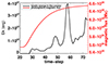 |
Fig. 1. Temporal evolution of the coronal kinetic energy calculated 3.2 Mm above the photosphere (black line) and of the photospheric magnetic flux (red line). Consecutive time-steps are 86.9 s apart. |
Fig. 2 contains slices of the temperature, vertical speed (Vz), and field-aligned current density, Jpar,

in the xz-midplane spanning the solar atmosphere (i.e. photosphere and above) for three snapshots during the simulation. Because the axis of the emerging flux tube runs along the y-axis, slices of physical parameters in the xz-midplane sample a cross-section perpendicular to and in the middle of the emerging flux tube axis. In the first row of Fig. 2, we show a snapshot during a standard jet, while the second and third row of this figure contain a snapshot of a pre-eruptive MFR and its eventual eruption into a blowout jet, respectively. The snapshot in the second row of Fig. 2 corresponds to a period of almost constant coronal kinetic energy (see Fig. 1), before it impulsively increases during an eruption associated with a blowout jet. We discuss this pre-eruptive MFR in more detail in Section 5. The standard jet (first row) corresponds to an extended region with high Vz values (panel (b)) that coincides with a high-temperature region (panel (a)). These are telltale signatures of standard jets that occur when reconnection between emerging closed and ambient open fields takes place. When these two sets of field lines start to reconnect, the heated plasma is emitted in the form of the standard jet. In the second row of Fig. 2, the cross-section of a pre-eruptive MFR can be traced by a quasi-circular concentration in Jpar (panel (f)), and it mainly contains cool plasma (panel (d)). The eruption of this MFR generates a large blowout jet (panel (h)) that contains both cool and hot plasma (panel (g)). Inspection of the associated movie also shows a multitude of quasi-steady upflows in addition to the larger-scale eruptions and jets.
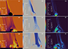 |
Fig. 2. Distribution of the logarithm of the temperature, Vz and Jpar (square-root scaling) in the xz-midplane spanning the solar atmosphere (i.e. photosphere and above) in the left, middle, and right column, respectively. Each row corresponds to a given snapshot during the simulation. Consecutive time-steps are 86.9 s apart. The associated movie is available online. |
In Fig. 3 we show the photospheric Bz for time-step 42. In this snapshot, a significant part of the flux emergence has taken place (see the photospheric magnetic flux evolution in Fig. 1). The PIL of the photospheric Bz (purple line) consists of two parts: one part between the two polarities of the emerging magnetic flux (inner PIL; iPIL) and the other part lies around the minority (negative) polarity emerging flux and essentially separates it from the ambient positive-polarity field. The photospheric imprint of the emerging magnetic flux tube consists of two components at either side of the iPIL: two oval-shaped strong-field spots, and two elongated weaker-field magnetic tails corresponding to the feet and the horizontal extensions of the emerging flux tube into the photosphere, respectively (e.g. López Fuentes et al. 2000; Archontis & Hood 2010; Luoni et al. 2011). Along most of the length of the iPIL, it separates spot-tail segments with a disparate magnetic field magnitude. However, around the centre of Fig. 3, and encompassed by the green box, lies a segment of the iPIL that features similar magnitude conjugate tail magnetic fields. As we show in the next section, the magnetic flux cancellation takes place in this region.
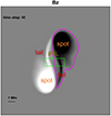 |
Fig. 3. Photospheric Bz for time-step 42. Black (white) corresponds to negative (positive) Bz saturated in ±300 Gauss. The purple line corresponds to the PIL of the photospheric Bz. The green box encapsulates the region in which magnetic flux cancellation takes place. |
4. Magnetic flux cancellation
4.1. Detection of magnetic flux cancellation
In this section, we discuss the signatures and characteristics of magnetic flux cancellation as they result from our simulation. Fig. 4 contains several representative panels of the photospheric Bz during the simulation, which can essentially be treated as photospheric Bz magnetograms. Each panel in this figure also includes the horizontal velocities of the photospheric magnetic footpoints, which are shown with blue arrows. In determining these velocities, we followed Démoulin & Berger (2003) and Lionello et al. (2020), who considered the impact of the flux emergence on the horizontal velocities of the magnetic footpoints (for an illustration of the effect, see, e.g., Figure 1 in Démoulin & Berger 2003). This is a necessary action to take, as we hereby use a flux-emergence simulation, and residing exclusively to the horizontal (plasma) velocities is not sufficient for the calculation of the magnetic-footpoints’ velocities.
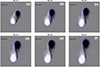 |
Fig. 4. Sample panels of the photospheric Bz and of the magnetic-footpoint horizontal speeds. Black (white) correspond to negative(positive) polarity Bz saturated in ±300 Gauss. The overplotted blue arrows correspond to the horizontal speeds of the magnetic footpoints. The longest arrows correspond to a magnitude of 1 km s−1. The purple line corresponds to the PIL of the photospheric Bz. The green box corresponds to the region in which magnetic flux cancellation takes place. Consecutive time-steps are 86.9 s apart. The associated movie is available online. |
Fig. 4 and the associated movie reveal several generic features of MHD simulations of emerging twisted flux tubes that lead to the formation of bipolar regions with strong PILs. This includes the appearance and development of conjugate magnetic spots and tails as well as complex flow fields with shear and rotation. The spots start to emerge at about time-step 23, and the tails appear slightly later, at about time-step 26. The Bz evolution in the green box (same as in Fig. 3) shows that during time-steps ≈20–35, the magnetic flux moves away from the iPIL due to the emerging and laterally expanding fields. However, at time-step ≈35, the segments of the conjugate tails inside the green box start to converge towards the iPIL and eventually reach a minimum distance at about time-step 53. The convergence of the magnetic tails is accompanied by a decrease in their magnetic field magnitude. The green box in Fig. 3 and Fig. 4 sufficiently covers the full length along the iPIL where the tail-tail convergence and interaction described above take place.
The magnetic footpoint velocities of Fig. 4 show an opposite rotation of the two spots, which drags the conjugate magnetic tails in opposite directions and hence shears them. These rotating and shearing motions result from Lorentz forces, as in many other MHD simulations and models (e.g. Longcope & Welsch 2000; Manchester 2001; Archontis & Török 2008; Fan 2009; Fang et al. 2012; Georgoulis et al. 2012; Leake et al. 2013; Sturrock et al. 2015; Syntelis et al. 2017). As the iPIL is inclined with respect to the x-axis, and because of the opposite-directed shearing footpoint motions on either side of the iPIL, we surmise that these motions introduce a component perpendicular to and pointing to the iPIL. This essentially causes the conjugate magnetic tails to converge to the iPIL.
To furthermore study the evolution of the conjugate magnetic tails, we generated Fig. 5, where we display a time-distance plot of Bz averaged along the height of the green box in Fig. 3 as a function of time and distance along the base of the box. During time-steps ≈23–35, we observe two diverging branches of opposite-signed Bz. Starting from time-step 35, however, the two branches start to converge and then attain a more or less constant distance at about time-step 53. The speed at which the two branches converge is around 1 km s−1 judged by the fiducial red line we supply in Fig. 5. These patterns are consistent with the photospheric magnetograms we discussed in the previous paragraphs.
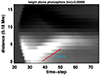 |
Fig. 5. Time-distance plot of the photospheric Bz corresponding to sums of Bz along the columns of the green box of Fig. 3; the distance corresponds to the position along the base of the box of Fig. 3. The inclined red line has a slope of ≈1 km s−1. Consecutive time-steps are 86.9 s apart. |
In Fig. 6 we show time-series of the positive, absolute negative, and net unsigned magnetic flux calculated for the green box in Fig. 3. This is equivalent to taking column sums of the time-distance plot in Fig. 5. We first note that the positive and negative fluxes are relatively well balanced. The positive flux is slightly higher as a natural consequence of the positive-polarity ambient magnetic field. From time-step 35 onward, which corresponds to the period of the conjugate-tail convergence and encounter discussed in the previous paragraphs, all fluxes decrease simultaneously. There is a significant decrease of ≈75% in the net unsigned magnetic flux during this period. This corresponds to a flux-cancellation rate of ≈3.2×10¹⁸ Mx hour−1 as resulting from the linear fit of the pertinent time-step and magnetic flux pairs (green line in Fig. 6). In shorter intervals that encompass major peaks in the coronal kinetic energy that correspond to eruptions and blowout jets, for example, from about time-steps 45–53 and 55–62 in Fig. 1, the magnetic flux decreases by about 15–20% of its value at the start of the corresponding intervals. In summary, Figures 3–6, and given the pertinent results presented in the Introduction, show telltale signatures of magnetic flux cancellation. This includes convergence followed by a decrease in their flux content in a PIL of photospheric magnetic patches of opposite polarity and similar magnetic field magnitude and flux.
 |
Fig. 6. Temporal evolution of the positive (blue line), negative (red line) and net unsigned photospheric magnetic flux (black line) in the green box of Fig. 3 shown from the appropriate column sums of the time-distance map of Fig. 5. The green line corresponds to a linear fit of the time-step and net unsigned flux pairs from time-step 35 onward. Consecutive time-steps are 86.9 s apart. |
Magnetic flux cancellation associated with conjugate magnetic tail fields can be traced up to ≈520 km above the photosphere. Above this height, the magnetic tails vanish because the magnetic field distribution becomes smoother, and moreover, the iPIL strongly shifts and is distorted with regard to its position and shape in the low photosphere. Fig. 7 shows an analog of Fig. 6, and the pertinent calculations were performed in the area enclosed by the green box in Fig. 3, but this time, located at a height of 3 pixels above the photosphere. As anticipated by the decrease with height of the magnetic field, the fluxes reported in this figure are lower than the corresponding photospheric fluxes in Fig. 6. Moreover, and as also noted in Fig. 6, all displayed fluxes (i.e. positive, absolute negative, and net unsigned) decrease at the same time, which is consistent with magnetic flux cancellation. However, we observe a delay of ≈7 time-steps (i.e. 608 s) in the onset of magnetic flux cancellation at z = 3 pixels as compared to z = 0 pixels. This delay is anticipated because we used a flux-emergence simulation in which magnetic flux progressively reaches larger heights in the solar atmosphere.
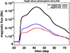 |
Fig. 7. Same as in Fig. 6, but this time, corresponding to magnetic fluxes calculated 520 km above the photosphere and in the same box as used for the calculations of Fig. 6. |
4.2. Interpretation of magnetic flux cancellation
In this section, we discuss the possible mechanism that causes the flux cancellation in our simulation. In Fig. 8 we display magnetic field lines traced from seeds within a sphere with a radius of 2 pixels that is centred 2 pixels above the centre of the photospheric plane of the simulation box, which is also the centre of the green box in Fig. 3. Therefore, these field lines essentially permeate the volume in which magnetic flux cancellation takes place. Fig. 8 shows two groups of magnetic field lines: J-shaped lines rooted in the magnetic tail and spots, and S-shaped field lines that are sandwiched between the J-shaped lines and run along the iPIL. The J-shaped field lines owe their shape to the twisting and shearing photospheric motions discussed in the previous paragraphs, which align them with the iPIL. They are carried by the converging magnetic footpoint motions to the iPIL (see, e.g. Fig. 4) where they eventually reconnect and give rise to the S-shaped field lines. The transition from J- to S-shaped field lines in PILs was frequently reported in both observational and modelling studies following the work of van Ballegooijen & Martens (1989), and we discuss this in more detail in Section 5. In tandem with the above, the conjugate tail magnetic fields associated with the J-shaped field lines undergoing reconnection in the iPIL also give rise to the (photospheric) magnetic flux-cancellation signatures discussed in the previous paragraphs. We therefore conclude that magnetic flux cancellation is associated with low-altitude magnetic reconnection between the J-shaped field lines.
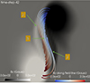 |
Fig. 8. Magnetic field lines traced from a sphere with a radius of 2 pixels and the centre 2 pixels above the middle of the photospheric plane of the simulation box for time-step 42. We display the photospheric Bz saturated in ±300 Gauss with a greyscale. The traced field lines are coloured as a function of Bz along their lengths. |
To elaborate on the nature of the magnetic flux cancellation reported here, we first calculated the component of Vz perpendicular to the magnetic field,  ,
,
where k corresponds to the unit vector along the positive z-axis. We opted to use  instead of Vz as the former only corresponds to the fraction of Vz perpendicular to the magnetic field. Therefore,
  can be viewed as a proxy of the vertical speed of the field lines and not of field-aligned plasma flows (see also Fang et al. 2012 for a discussion of field line speeds with regard to magnetic flux cancellation). A positive (negative)
  implies that the corresponding field line segment rises (falls).
We also calculated the component of the magnetic tension vector (∼B·∇B) along the z-axis, κz, normalised by the field magnitude,
κz with positive (negative) sign corresponds to field lines that are locally concave upward (downward). Regions in photospheric PILs with positive κz correspond to the so-called bald patches (Titov et al. 1993).
In panels (a) and (b) of Fig. 9, we show an overhead and a side view of the S-shaped field lines in Fig. 8 coloured as a function of  along their length. We conclude that the S-shaped field lines generally correspond to positive
  with a magnitude of ≈0.2–0.5 km s−1. We assert that the central parts of the S-shaped field lines, that is, those corresponding to the green box in Fig. 3 in which magnetic flux cancellation takes place, have positive κz. Therefore, from the analysis of
  and κz, we conclude that the field lines slowly rise and are concave-upward in their middle in the region in which flux cancellation takes place. This is equivalent to emerging U-loops associated with magnetic flux cancellation discussed in the Introduction. In summary, and from the analysis of Figures 8 and 9, we suggest that reconnection of the J-shaped field lines rooted in the conjugate tails at either side of the iPIL gives rise to concave-upward slowly rising magnetic field lines. The latter explains the reduction in the photospheric magnetic flux that is associated with magnetic flux cancellation.
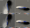 |
Fig. 9. S-shaped magnetic field lines of Fig. 8 coloured as a function of |

As discussed in the Introduction, magnetic reconnection associated with magnetic flux cancellation can lead to emerging (submerging) U- and Ω-loops. The emerging U-loops are consistent with the rising concave-upward field lines discussed in the previous paragraph. To provide a tentative explanation for the lack of submerging Ω-loops, we followed van Ballegooijen & Martens (1989). They suggested that post-reconnection field lines in flux-cancellation sites can submerge when they are only short enough for the associated magnetic curvature to overcome the corresponding magnetic buoyancy. This requirement is consistent with a maximum footpoint separation of ≈900 km, which is a few times the photospheric scale-height, for submergence to occur. Assuming semicircular field lines, we obtain an equivalent maximum field line length of ≈1300 km. Finally, calculation of the lengths of the S-shaped field lines of Fig. 9 gives values in the range ≈3300–4800 km, which might explain why we did not obtain submerging field lines. This is confirmed in Fig. 10. This figure contains the time-series of the positive, absolute negative, and net unsigned magnetic flux for the green box in Fig. 3 in which we detected photospheric magnetic flux cancellation, this time at a depth of 180 km below the photosphere. Fig. 10 clearly shows no increase in the relevant subphotospheric magnetic fluxes during the period when magnetic flux cancellation is observed in the photosphere. This increase would be expected if the cancellation were caused by the submergence of magnetic field lines.
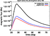 |
Fig. 10. Temporal evolution of the positive (blue line) and negative (red line) magnetic flux 180 km below the photosphere for the green box of Fig. 3. Consecutive time-steps are 86.9 s apart. |
4.3. Magnetic flux cancellation and pre-eruptive MFRs
We now discuss the implications of our results in terms of pre-eruptive magnetic configurations. Following our discussion of Fig. 8 in terms of the J- and S-shaped magnetic field lines, we note that the overall behaviour adheres to the so-called arcade-to-sigmoid transformation scenario originally advocated by van Ballegooijen & Martens (1989), which is a basic element of a number of observational and theoretical and modelling works. According to this scenario, magnetic reconnection converts J-shaped field (arcade) field lines into S-shaped (sigmoid) field lines, which eventually leads to the formation of pre-eruptive MFRs. The S-shaped field lines in Fig. 8 do not correspond to a fully developed MFR, but they rather represent a seed thereof. Additional reconnection in the iPIL is required to generate truly twisted field lines undergoing several crossings of the iPIL, and hence, eventually, of pre-eruptive MFRs as well (see, e.g. the schematics and associated discussion by van Ballegooijen & Martens 1989 and Green et al. 2011). This reconnection does not only lead to the formation of pre-eruptive MFRs, but also contributes to their subsequent growth (see also the pertinent MHD simulation results by e.g. Aulanier et al. 2010; Syntelis et al. 2017).
To draw a more quantitative link between magnetic flux cancellation and pre-eruptive MFRs, we discuss the pre-eruptive MFR in Fig. 11. This MFR corresponds to the yellow field lines that were traced from a quasi-circular Jpar concentration in the xz-midplane outlined with the dashed line. The Jpar concentration used for the MFR field line tracing sits at the top of a narrow vertical Jpar concentration that is permeated with the purple magnetic field lines traced from the magnetic flux-cancellation region, as discussed for Fig. 8. We calculated the twist number, Tw, of these field lines,
where the integration was performed along the length L of each of the traced field lines. Tw essentially supplies the number of turns that two infinitesimally adjacent field lines make around each other (Berger & Prior 2006). We used the software described by Liu et al. (2016) in our calculations of Tw. The average Tw of the yellow field lines is 1.2, and the corresponding standard deviation is 0.5. Hence, this MFR is a weakly twisted MFR, as are most of the pre-eruptive MFRs reported by either observations or models (e.g. Patsourakos et al. 2020). We recall that this MFR eventually erupted and gave rise to a blowout jet (see, e.g. the discussion of Fig. 2).
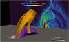 |
Fig. 11. Pre-eruptive MFR (yellow magnetic field lines) traced from a small sphere centred at and spanning a quasi-circular concentration of enhanced Jpar outlined with dashes in the xz-midplane. The Jpar distribution in the xz-midplane is translated from its original position for clarity. The purple magnetic field lines are traced from the same seeds as the field lines shown in Fig. 8. We display the photospheric Bz distribution with a greyscale. The figure corresponds to time-step 53. |
We now calculated an estimate of the axial, that is, associated with By, magnetic flux, Φy, of the pre-eruptive MFR. In calculating Φy, we considered pixels inside the Jpar concentration used to trace the MFR field lines. The resulting Φy is 4.2×10¹⁸ Mx, while the cancelled magnetic flux in the interval encompassing the associated eruption and blowout jet, that is, spanning time-steps 53–63 (see Fig. 1), is about 1018 Mx. This means that magnetic flux cancellation might have roughly contributed up to ≈ the 25% of the axial magnetic flux of the pre-eruptive MFR. Following the discussion of the previous paragraphs, the magnetic flux associated with flux cancellation may have ended up in the pre-eruptive MFR as a consequence of multiple reconnections that lifted and coiled the original S-shaped field lines. For an in-depth analysis of the connection between the magnetic fluxes associated with magnetic flux cancellation and those sealed in pre-eruptive MFRs and its intricacies, we refer to Green et al. (2011). It is obvious from the above that the cancelled magnetic flux is neither the sole nor the main contributor to the magnetic flux content of the pre-eruptive MFR. Reconnection and cancellation above the photospheric layers in which we observed magnetic flux cancellation might have been relevant, as shown, for example by Aulanier et al. (2010), Syntelis et al. (2017). As discussed previously, beyond a certain height in the low photosphere, the magnetic tails vanish and the magnetic field distribution becomes more homogeneous. This might in principle facilitate magnetic reconnection and magnetic flux cancellation along more extended segments in the respective iPILs. Calculating the contribution of reconnection and cancellation in multiple heights above the photosphere in the magnetic flux budget of pre-eruptive MFRs is a worthwhile future investigation.
5. Conclusions and discussion
We have presented a study of magnetic flux cancellation in a 3D MHD simulation of the emergence of a twisted flux tube into a coronal hole that led to eruptions and jets. Our main conclusions are summarised below.
-
We found photospheric magnetic flux cancellation between opposite-polarity and commensurate strength magnetic flux patches entrained in the magnetic tails of the emerging system.
-
The cancelling patches are associated with J-shaped (sheared) field lines, which converge and eventually reconnect along a short segment of the iPIL. The reconnection events generate slowly rising concave-upward field lines that lead to the flux decrease associated with magnetic flux cancellation.
-
The magnetic flux cancellation rate is ≈3.2×10¹⁸ Mx hour−1. Time periods when magnetic flux decreases by 15–20% were found during intervals encompassing individual eruptions and jets.
-
Magnetic flux cancellation is not temporally correlated with the standard jets of the simulation, but occurs when the system experiences eruptions and blowout jets.
-
Magnetic flux cancellation can be traced to 520 km above the photosphere, with a delay of of around 10 minutes with respect to its occurrence in the photosphere.
-
Magnetic flux cancellation might have been relevant to the formation of MFR seeds, which eventually grow and erupt and give rise to the blowout jets of the simulation.
Our simulations included partial ionisation of hydrogen in the low solar atmosphere. Whether this inclusion affects magnetic flux cancellation in flux-emergence simulations requires further work. We recall, however, that a handful of MHD simulations of emerging twisted flux tubes employing full ionisation of hydrogen indeed exhibited evidence of magnetic flux cancellation as well, but no eruptive behaviour was reported (Magara 2011; Fang et al. 2012).
We first compared our results with the pertinent MHD flux-emergence simulations of Magara (2011) and Fang et al. (2012). As also discussed in the Introduction, both studies involved the emergence of twisted flux tubes from the convection zone into the solar atmosphere, and both gave rise to magnetic flux cancellation. Similarly to our results, these studies both involved slowly rising concave-upward field lines assuming the form of U-loops. Magara (2011) reported that the U-loops corresponded to the bottom of the emerging flux tube, which can rise because their curvature is small. Fang et al. (2012) reported that the U-loops resulted from magnetic reconnection driven by convective and shear motions. Therefore, our results agree better with those by Fang et al. (2012).
We now compare our results with observations. We first compare the deduced magnetic cancellation rate, that is, 3.2×10¹⁸ Mx hour−1, with pertinent observational results. Panesar et al. (2018) found from HMI magnetograms an average magnetic flux-cancellation rate ≈0.6×10¹⁸ Mx hour−1 for 13 ECH jets, which is significantly lower than our findings. Reid et al. (2016) inferred magnetic flux-cancellation rates associated with Ellerman bombs inside an active region in the range ≈3.6×(1017−1018) Mx hour−1. Kaithakkal & Solanki (2019) found a magnetic flux-cancellation rate of ≈3.6×10¹⁸ Mx hour−1 in a young active region. Ledvina et al. (2022) found a magnetic flux-cancellation rate of ≈1.4×10¹⁸ Mx hour−1 for 38 QS magnetic flux-cancellation events. Wang et al. (2022) analysed 1245 magnetic flux-cancellation events inside an ECH and found an average magnetic flux-cancellation rate of ≈1018 Mx hour−1. Interestingly, a common element in Reid et al. (2016), Kaithakkal & Solanki (2019), Ledvina et al. (2022) and Wang et al. (2022) that led to elevated magnetic flux-cancellation rates which are closer with our results is that they all employed high-resolution magnetograms with a sub-arcesecond spatial resolution. We recall that the (horizontal) spatial resolution of our simulation of 180 km corresponds to scales that can be resovled with sub-arcsecond resolution observations, that is, they are below the spatial resolution of HMI. This implies that a simulation output at a spatial resolution commensurate to that of HMI could lead to lower magnetic flux-cancellation rates that are more consistent with HMI observations. The speed of the converging motions of the magnetic tails associated with magnetic flux cancellation of our simulation (i.e. ≈1km s−1) is consistent with observations in magnetic flux cancellation sites corresponding to speeds in the range 0.3–1.8 km s−1 (e.g. Kaithakkal & Solanki 2019; Ledvina et al. 2022). Panesar et al. (2018) found decreases of 21–73% in the magnetic flux during temporal intervals around 13 ECH jets; the lower value of their values is consistent with the largest decrease (that is ≈20%) found in our simulation. Finally, our simulation results showing that blowout jets occur only during periods of magnetic flux cancellation, are consistent with a number of observational works discussed in the Introduction (McGlasson et al. 2017; Mou et al. 2018; Panesar et al. 2018, 2023; Moore et al. 2022). However, we have also discussed observational works in the Introduction showing the contrary (Kumar et al. 2019; Muglach 2021). We note here that not all of the jets of our simulation, and namely the standard jets, occurred when magnetic flux cancellation was occurring. Summarizing, it seems as if our simulation is consistent with several properties of magnetic flux cancellation and coronal jets and eruptions reported by observations.
An interesting result of our study is that magnetic flux cancellation can be traced, with a temporal delay of the order of about 10 minutes, in multiple heights up to ≈520 km above the photosphere. The vertical extent of the magnetic cancellation region is associated with the respective vertical extent of the magnetic tails. Multi-height high-resolution observations of Bz, for example with the Daniel K. Inouye Solar Telescope (DKIST) (e.g. de Wijn et al. 2022) and with the Swedish Solar Telescope (SST) Gošić et al. (2018, 2024) might supply important tests of these predictions based on our modelling.
While our simulation is consistent with several basic aspects of magnetic flux-cancellation observations, it also gives rise to a major difference. That is, the magnetic flux undergoing cancellation (e.g. Fig. 6) is significantly lower by about a factor of 100 with respect to the magnetic flux budget in the photospheric layer of the entire simulation box (e.g. Fig. 1), which is essentially dominated by the emergence of the twisted flux tube. This difference can readily be understood in terms of the small field of view of our calculations of the magnetic flux cancellation, that is, the green box in Fig. 3. In retrospective, if we had used a larger box than the green box in Fig. 3 to monitor the evolution of magnetic flux, we would have missed the signature of magnetic flux cancellation, that is, the magnetic flux evolution of Fig. 6.
While opposite-polarity magnetic fields converge towards the iPIL along its entire length, with the exception of the fields inside the green box in Fig. 3 and for the most part of the considered temporal interval, they correspond to largely disparate magnetic-field magnitudes, that is, to spot-tail magnetic fields. The interaction of these disparate magnitude fields may lead to the so-called unbalanced flux cancellation discussed by DeForest et al. (2007), which does not agree with the archetypal notion for flux cancellation, however, which involves opposite-polarity and similar-magnitude magnetic fields. A potential application of unbalanced magnetic flux cancellation in our simulation could be found during the standard jets in the external PIL of the system between the emerging and stronger negative flux (spot) and the ambient and weaker surrounding positive fields (e.g. see Fig. 3). Our calculation of the magnetic flux evolution in boxes bounding these fields only showed a decrease in the positive magnetic flux during the standard jets, while the negative magnetic fluxes continued to increase. However, as amply demonstrated in the existing literature on jets (see, e.g. the related literature in the Introduction) magnetic reconnection above the photosphere is the key physical mechanism behind standard jets. It therefore seems rather hard to attribute the triggering of the (global) eruptions and jets of our simulation to magnetic flux cancellation. This is corroborated by MHD simulations of larger-scale eruptions that suggest that the cancelled magnetic flux is a significant fraction of the total available magnetic flux, for example 6–11% in the studies by Archontis & Hood (2010), Aulanier et al. (2010), Hassanin et al. (2022). The same constraint also follows from observations (e.g. Panesar et al. 2018), showing that a sizeable fraction of the available magnetic flux in sites in which coronal jets occur undergoes cancellation. Because magnetic flux cancellation does not seem to be a plausible trigger mechanism of the jets and eruptions of our simulation, other proposed mechanisms therefore need to be studied (e.g. Pariat et al. 2009; Wyper et al. 2017). This task is beyond the scope of our study, however.
The important caveat of our simulation in terms of the small fraction of the available magnetic flux involved in magnetic flux cancellation may be mitigated in future MHD modelling efforts in at least two ways. First, by enhancing the magnitude of the ambient magnetic field in a number of locations. This emulates unipolar enhanced magnetic field patches in coronal holes, that is, an enhanced network, which could cancel the minority polarity field of the emerging bipoles (e.g. Panesar et al. 2018; Moore et al. 2022). Second, by considering the emergence and interaction of multiple twisted flux tubes (e.g. Lee et al. 2015; Chintzoglou et al. 2019). Both scenarios might lead to the encounter and eventual annihilation of large patches of opposite-polarity magnetic fields, and might therefore increase the fraction of the available magnetic flux undergoing magnetic flux cancellation. Finally, it will be worthwhile to investigate which properties of single emerging twisted flux tubes such as geometry and twist distribution might be more prone to lead to magnetic flux cancellation.
Data availability
Movies associated to Figs 2 and 4 are available at https://www.aanda.org
Acknowledgments
The authors acknowledge support by the ERC Synergy Grant ‘Whole Sun’ (GAN: 810218). The authors extend sincere thanks to the referee for useful suggestions and comments on the manuscript.
References
- Amari, T., Luciani, J. F., Aly, J. J., Mikic, Z., & Linker, J. 2003, ApJ, 595, 1231 [Google Scholar]
- Arber, T. D., Longbottom, A. W., Gerrard, C. L., & Milne, A. M. 2001, J. Comput. Phys., 171, 151 [NASA ADS] [CrossRef] [Google Scholar]
- Archontis, V., & Hood, A. W. 2010, A&A, 514, A56 [NASA ADS] [CrossRef] [EDP Sciences] [Google Scholar]
- Archontis, V., & Hood, A. W. 2013, ApJ, 769, L21 [Google Scholar]
- Archontis, V., & Syntelis, P. 2019, Philos. Trans. R. Soc. Lond. Ser. A, 377, 20180387 [Google Scholar]
- Archontis, V., & Török, T. 2008, A&A, 492, L35 [NASA ADS] [CrossRef] [EDP Sciences] [Google Scholar]
- Aulanier, G., Török, T., Démoulin, P., & DeLuca, E. E. 2010, ApJ, 708, 314 [Google Scholar]
- Bellot Rubio, L. R., & Beck, C. 2005, ApJ, 626, L125 [Google Scholar]
- Berger, M. A., & Prior, C. 2006, J. Phys. A: Math. Gen., 39, 8321 [Google Scholar]
- Bernasconi, P. N., Rust, D. M., Georgoulis, M. K., & Labonte, B. J. 2002, Sol. Phys., 209, 119 [NASA ADS] [CrossRef] [Google Scholar]
- Chae, J., Moon, Y. -J., & Pevtsov, A. A. 2004, ApJ, 602, L65 [Google Scholar]
- Chen, P. F. 2011, Living Rev. Sol. Phys., 8, 1 [Google Scholar]
- Chintzoglou, G., Zhang, J., Cheung, M. C. M., & Kazachenko, M. 2019, ApJ, 871, 67 [NASA ADS] [CrossRef] [Google Scholar]
- Chitta, L. P., Zhukov, A. N., Berghmans, D., et al. 2023, Science, 381, 867 [NASA ADS] [CrossRef] [Google Scholar]
- Chouliaras, G., & Archontis, V. 2025, ApJ, 979, 53 [Google Scholar]
- Chouliaras, G., Syntelis, P., & Archontis, V. 2023, ApJ, 952, 21 [NASA ADS] [CrossRef] [Google Scholar]
- DeForest, C. E., Hagenaar, H. J., Lamb, D. A., Parnell, C. E., & Welsch, B. T. 2007, ApJ, 666, 576 [NASA ADS] [CrossRef] [Google Scholar]
- Démoulin, P., & Berger, M. A. 2003, Sol. Phys., 215, 203 [CrossRef] [Google Scholar]
- de Wijn, A. G., Casini, R., Carlile, A., et al. 2022, Sol. Phys., 297, 22 [NASA ADS] [CrossRef] [Google Scholar]
- Færder, Ø. H., Nóbrega-Siverio, D., & Carlsson, M. 2023, A&A, 675, A97 [NASA ADS] [CrossRef] [EDP Sciences] [Google Scholar]
- Fan, Y. 2009, ApJ, 697, 1529 [NASA ADS] [CrossRef] [Google Scholar]
- Fang, F., Manchester, W. I., Abbett, W. P., & van der Holst, B. 2012, ApJ, 754, 15 [NASA ADS] [CrossRef] [Google Scholar]
- Fang, F., Fan, Y., & McIntosh, S. W. 2014, ApJ, 789, L19 [NASA ADS] [CrossRef] [Google Scholar]
- Georgoulis, M. K., Titov, V. S., & Mikić, Z. 2012, ApJ, 761, 61 [NASA ADS] [CrossRef] [Google Scholar]
- Georgoulis, M. K., Li, Q., Lee, Q., Wang, H., & Raouafi, N. E. 2025, ApJ, submitted [Google Scholar]
- Gošić, M., de la Cruz Rodríguez, J., De Pontieu, B., et al. 2018, ApJ, 857, 48 [CrossRef] [Google Scholar]
- Gošić, M., De Pontieu, B., & Sainz Dalda, A. 2024, ApJ, 964, 175 [Google Scholar]
- Green, L. M., & Kliem, B. 2009, ApJ, 700, L83 [NASA ADS] [CrossRef] [Google Scholar]
- Green, L. M., Kliem, B., & Wallace, A. J. 2011, A&A, 526, A2 [NASA ADS] [CrossRef] [EDP Sciences] [Google Scholar]
- Green, L. M., Török, T., Vršnak, B., Manchester, W., & Veronig, A. 2018, Space Sci. Rev., 214, 46 [Google Scholar]
- Harvey, K. L., Jones, H. P., Schrijver, C. J., & Penn, M. J. 1999, Sol. Phys., 190, 35 [NASA ADS] [CrossRef] [Google Scholar]
- Hassanin, A., Kliem, B., Seehafer, N., & Török, T. 2022, ApJ, 929, L23 [Google Scholar]
- Kaithakkal, A. J., & Solanki, S. K. 2019, A&A, 622, A200 [NASA ADS] [CrossRef] [EDP Sciences] [Google Scholar]
- Koletti, M., Gontikakis, C., Patsourakos, S., & Tsinganos, K. 2024, A&A, 690, A11 [NASA ADS] [CrossRef] [EDP Sciences] [Google Scholar]
- Kumar, P., Karpen, J. T., Antiochos, S. K., et al. 2019, ApJ, 873, 93 [NASA ADS] [CrossRef] [Google Scholar]
- Kumar, P., Karpen, J. T., Antiochos, S. K., et al. 2021, ApJ, 907, 41 [Google Scholar]
- Leake, J. E., Linton, M. G., & Török, T. 2013, ApJ, 778, 99 [NASA ADS] [CrossRef] [Google Scholar]
- Ledvina, V. E., Kazachenko, M. D., Criscuoli, S., et al. 2022, ApJ, 934, 38 [CrossRef] [Google Scholar]
- Lee, E. J., Archontis, V., & Hood, A. W. 2015, ApJ, 798, L10 [Google Scholar]
- Lionello, R., Titov, V. S., Mikić, Z., & Linker, J. A. 2020, ApJ, 891, 14 [Google Scholar]
- Liu, R., Kliem, B., Titov, V. S., et al. 2016, ApJ, 818, 148 [Google Scholar]
- Livi, S. H. B., Wang, J., & Martin, S. F. 1985, Aust. J. Phys., 38, 855 [Google Scholar]
- Longcope, D. W., & Welsch, B. T. 2000, ApJ, 545, 1089 [NASA ADS] [CrossRef] [Google Scholar]
- López Fuentes, M. C., Demoulin, P., Mandrini, C. H., & van Driel-Gesztelyi, L. 2000, ApJ, 544, 540 [CrossRef] [Google Scholar]
- Luoni, M. L., Démoulin, P., Mandrini, C. H., & van Driel-Gesztelyi, L. 2011, Sol. Phys., 270, 45 [NASA ADS] [CrossRef] [Google Scholar]
- Mackay, D. H., & van Ballegooijen, A. A. 2006, ApJ, 641, 577 [NASA ADS] [CrossRef] [Google Scholar]
- Magara, T. 2011, PASJ, 63, 417 [Google Scholar]
- Manchester, W. I. 2001, ApJ, 547, 503 [Google Scholar]
- Martin, S. F. 1988, Sol. Phys., 117, 243 [NASA ADS] [CrossRef] [Google Scholar]
- Martin, S. F., Livi, S. H. B., & Wang, J. 1985, Aust. J. Phys., 38, 929 [Google Scholar]
- McGlasson, R., Panesar, N. K., Sterling, A. C., & Schm, R. L. 2017, AGU Fall Meeting Abstracts, 2017, SH43A–2796 [Google Scholar]
- Moore, R. L., Sterling, A. C., Hudson, H. S., & Lemen, J. R. 2001, ApJ, 552, 833 [Google Scholar]
- Moore, R. L., Cirtain, J. W., Sterling, A. C., & Falconer, D. A. 2010, ApJ, 720, 757 [Google Scholar]
- Moore, R. L., Panesar, N. K., Sterling, A. C., & Tiwari, S. K. 2022, ApJ, 933, 12 [Google Scholar]
- Moraitis, K., Archontis, V., & Chouliaras, G. 2024, A&A, 690, A181 [NASA ADS] [CrossRef] [EDP Sciences] [Google Scholar]
- Moreno-Insertis, F., & Galsgaard, K. 2013, ApJ, 771, 20 [Google Scholar]
- Moreno-Insertis, F., Galsgaard, K., & Ugarte-Urra, I. 2008, ApJ, 673, L211 [Google Scholar]
- Mou, C., Madjarska, M. S., Galsgaard, K., & Xia, L. 2018, A&A, 619, A55 [NASA ADS] [CrossRef] [EDP Sciences] [Google Scholar]
- Muglach, K. 2021, ApJ, 909, 133 [NASA ADS] [CrossRef] [Google Scholar]
- Nelson, C. J., Hayes, L. A., Müller, D., et al. 2024, A&A, 692, A236 [NASA ADS] [CrossRef] [EDP Sciences] [Google Scholar]
- Nindos, A., Patsourakos, S., Moraitis, K., et al. 2024, A&A, 689, L11 [NASA ADS] [CrossRef] [EDP Sciences] [Google Scholar]
- Nóbrega-Siverio, D., & Moreno-Insertis, F. 2022, ApJ, 935, L21 [CrossRef] [Google Scholar]
- Nóbrega-Siverio, D., Moreno-Insertis, F., & Martínez-Sykora, J. 2016, ApJ, 822, 18 [Google Scholar]
- Nóbrega-Siverio, D., Cabello, I., Bose, S., et al. 2024, A&A, 686, A218 [NASA ADS] [CrossRef] [EDP Sciences] [Google Scholar]
- Panesar, N. K., Sterling, A. C., & Moore, R. L. 2018, ApJ, 853, 189 [NASA ADS] [CrossRef] [Google Scholar]
- Panesar, N. K., Hansteen, V. H., Tiwari, S. K., et al. 2023, ApJ, 943, 24 [NASA ADS] [CrossRef] [Google Scholar]
- Pariat, E., Antiochos, S. K., & DeVore, C. R. 2009, ApJ, 691, 61 [Google Scholar]
- Patsourakos, S., Vourlidas, A., Török, T., et al. 2020, Space Sci. Rev., 216, 131 [Google Scholar]
- Pontin, D. I., Priest, E. R., Chitta, L. P., & Titov, V. S. 2024, ApJ, 960, 51 [NASA ADS] [CrossRef] [Google Scholar]
- Raouafi, N. E., Patsourakos, S., Pariat, E., et al. 2016, Space Sci. Rev., 201, 1 [Google Scholar]
- Raouafi, N. E., Stenborg, G., Seaton, D. B., et al. 2023, ApJ, 945, 28 [NASA ADS] [CrossRef] [Google Scholar]
- Reid, A., Mathioudakis, M., Doyle, J. G., et al. 2016, ApJ, 823, 110 [Google Scholar]
- Rempel, M., Chintzoglou, G., Cheung, M. C. M., Fan, Y., & Kleint, L. 2023, ApJ, 955, 105 [NASA ADS] [CrossRef] [Google Scholar]
- Savcheva, A. S., Green, L. M., van Ballegooijen, A. A., & DeLuca, E. E. 2012, ApJ, 759, 105 [NASA ADS] [CrossRef] [Google Scholar]
- Schmieder, B. 2022, Front. Astron. Space Sci., 9, 820183 [NASA ADS] [CrossRef] [Google Scholar]
- Shen, Y. 2021, Proc. R. Soc. Lond. Ser. A, 477, 217 [NASA ADS] [Google Scholar]
- Sterling, A. C., Moore, R. L., Falconer, D. A., & Adams, M. 2015, Nature, 523, 437 [NASA ADS] [CrossRef] [Google Scholar]
- Sturrock, Z., Hood, A. W., Archontis, V., & McNeill, C. M. 2015, A&A, 582, A76 [NASA ADS] [CrossRef] [EDP Sciences] [Google Scholar]
- Syntelis, P., Archontis, V., & Tsinganos, K. 2017, ApJ, 850, 95 [NASA ADS] [CrossRef] [Google Scholar]
- Syntelis, P., Priest, E. R., & Chitta, L. P. 2019, ApJ, 872, 32 [NASA ADS] [CrossRef] [Google Scholar]
- Takizawa, K., Kitai, R., & Zhang, Y. 2012, Sol. Phys., 281, 599 [Google Scholar]
- Titov, V. S., Priest, E. R., & Demoulin, P. 1993, A&A, 276, 564 [NASA ADS] [Google Scholar]
- van Ballegooijen, A. A., & Martens, P. C. H. 1989, ApJ, 343, 971 [Google Scholar]
- van Driel-Gesztelyi, L., Malherbe, J. M., & Démoulin, P. 2000, A&A, 364, 845 [Google Scholar]
- Wang, J., Lee, J., Liu, C., Cao, W., & Wang, H. 2022, ApJ, 924, 137 [NASA ADS] [CrossRef] [Google Scholar]
- Wyper, P. F., Antiochos, S. K., & DeVore, C. R. 2017, Nature, 544, 452 [Google Scholar]
- Xing, C., Aulanier, G., Cheng, X., Xia, C., & Ding, M. 2024, ApJ, 966, 70 [Google Scholar]
- Yang, S., Zhang, J., & Borrero, J. M. 2009, ApJ, 703, 1012 [NASA ADS] [CrossRef] [Google Scholar]
- Yardley, S. L., Green, L. M., van Driel-Gesztelyi, L., Williams, D. R., & Mackay, D. H. 2018, ApJ, 866, 8 [Google Scholar]
- Yokoyama, T., & Shibata, K. 1996, PASJ, 48, 353 [Google Scholar]
- Zwaan, C. 1987, ARA&A, 25, 83 [NASA ADS] [CrossRef] [Google Scholar]
All Figures
|
Fig. 1. Temporal evolution of the coronal kinetic energy calculated 3.2 Mm above the photosphere (black line) and of the photospheric magnetic flux (red line). Consecutive time-steps are 86.9 s apart. |
| In the text | |
|
Fig. 2. Distribution of the logarithm of the temperature, Vz and Jpar (square-root scaling) in the xz-midplane spanning the solar atmosphere (i.e. photosphere and above) in the left, middle, and right column, respectively. Each row corresponds to a given snapshot during the simulation. Consecutive time-steps are 86.9 s apart. The associated movie is available online. |
| In the text | |
|
Fig. 3. Photospheric Bz for time-step 42. Black (white) corresponds to negative (positive) Bz saturated in ±300 Gauss. The purple line corresponds to the PIL of the photospheric Bz. The green box encapsulates the region in which magnetic flux cancellation takes place. |
| In the text | |
|
Fig. 4. Sample panels of the photospheric Bz and of the magnetic-footpoint horizontal speeds. Black (white) correspond to negative(positive) polarity Bz saturated in ±300 Gauss. The overplotted blue arrows correspond to the horizontal speeds of the magnetic footpoints. The longest arrows correspond to a magnitude of 1 km s−1. The purple line corresponds to the PIL of the photospheric Bz. The green box corresponds to the region in which magnetic flux cancellation takes place. Consecutive time-steps are 86.9 s apart. The associated movie is available online. |
| In the text | |
|
Fig. 5. Time-distance plot of the photospheric Bz corresponding to sums of Bz along the columns of the green box of Fig. 3; the distance corresponds to the position along the base of the box of Fig. 3. The inclined red line has a slope of ≈1 km s−1. Consecutive time-steps are 86.9 s apart. |
| In the text | |
|
Fig. 6. Temporal evolution of the positive (blue line), negative (red line) and net unsigned photospheric magnetic flux (black line) in the green box of Fig. 3 shown from the appropriate column sums of the time-distance map of Fig. 5. The green line corresponds to a linear fit of the time-step and net unsigned flux pairs from time-step 35 onward. Consecutive time-steps are 86.9 s apart. |
| In the text | |
|
Fig. 7. Same as in Fig. 6, but this time, corresponding to magnetic fluxes calculated 520 km above the photosphere and in the same box as used for the calculations of Fig. 6. |
| In the text | |
|
Fig. 8. Magnetic field lines traced from a sphere with a radius of 2 pixels and the centre 2 pixels above the middle of the photospheric plane of the simulation box for time-step 42. We display the photospheric Bz saturated in ±300 Gauss with a greyscale. The traced field lines are coloured as a function of Bz along their lengths. |
| In the text | |
|
Fig. 9. S-shaped magnetic field lines of Fig. 8 coloured as a function of |
| In the text | |
|
Fig. 10. Temporal evolution of the positive (blue line) and negative (red line) magnetic flux 180 km below the photosphere for the green box of Fig. 3. Consecutive time-steps are 86.9 s apart. |
| In the text | |
|
Fig. 11. Pre-eruptive MFR (yellow magnetic field lines) traced from a small sphere centred at and spanning a quasi-circular concentration of enhanced Jpar outlined with dashes in the xz-midplane. The Jpar distribution in the xz-midplane is translated from its original position for clarity. The purple magnetic field lines are traced from the same seeds as the field lines shown in Fig. 8. We display the photospheric Bz distribution with a greyscale. The figure corresponds to time-step 53. |
| In the text | |
Current usage metrics show cumulative count of Article Views (full-text article views including HTML views, PDF and ePub downloads, according to the available data) and Abstracts Views on Vision4Press platform.
Data correspond to usage on the plateform after 2015. The current usage metrics is available 48-96 hours after online publication and is updated daily on week days.
Initial download of the metrics may take a while.