| Issue |
A&A
Volume 699, July 2025
|
|
|---|---|---|
| Article Number | A261 | |
| Number of page(s) | 13 | |
| Section | Planets, planetary systems, and small bodies | |
| DOI | https://doi.org/10.1051/0004-6361/202554481 | |
| Published online | 16 July 2025 | |
Enforcing multiple constraints on the interior structure of Ganymede: A machine learning approach
1
Dipartimento di Fisica e Astronomia “Galileo Galilei”, Università di Padova,
Vicolo dell’Osservatorio 3,
35122
Padova,
Italy
2
Centro di Ateneo di Studi e Attività Spaziali “Giuseppe Colombo” (CISAS),
Via Venezia 15,
35131
Padova,
Italy
★ Corresponding author: This email address is being protected from spambots. You need JavaScript enabled to view it.
Received:
11
March
2025
Accepted:
3
June
2025
Abstract
Determining the internal composition of planetary bodies remains a challenging problem due to observational degeneracies. In the 2030s, ESA’s Juice mission will orbit Ganymede and provide key constraints on its interior structure, including estimates of the polar moment of inertia, Love numbers, libration amplitudes, and the amplitude and phase of the induced magnetic field due to a subsurface ocean. To impose these constraints in the most effective way, a joint inversion of all available parameters would be ideal. In this work, we applied a machine learning approach to predict the thicknesses and densities of Ganymede’s internal layers, the viscosity of the icy shell, and the ocean conductivity from these observables. We generated a synthetic dataset of plausible internal structures via Monte Carlo sampling and computed the corresponding observables using existing physical models. A neural network was then trained to learn the intricate relationships between them. The trained model retrieves the internal structure parameters with varying degrees of accuracy across different layers. It performs well in predicting the thicknesses and densities of the icy shell and ocean, with mean absolute errors on the order of 10 km and 10 kg m−3, respectively. These errors increase to about 40 km and 20 kg m−3 for the high-pressure ice layer beneath the ocean. The trained model also estimates the shell viscosity with a mean absolute error of 0.05 log10 Pa s, and the ocean conductivity with an error of 0.1 S m−1. However, the neural network performs poorly in the task of inferring the thickness and density of the deeper interior, suggesting limited sensitivity of these parameters to the chosen set of observables. The Monte Carlo dropout method was utilized to estimate the uncertainties in the predicted parameters. These results highlight the potential of machine learning as a fast, preliminary tool for detecting families of internal structures compatible with the observed parameters.
Key words: methods: numerical / planets and satellites: composition / planets and satellites: interiors / planets and satellites: oceans / planets and satellites: individual: Ganymede
© The Authors 2025
 Open Access article, published by EDP Sciences, under the terms of the Creative Commons Attribution License (https://creativecommons.org/licenses/by/4.0), which permits unrestricted use, distribution, and reproduction in any medium, provided the original work is properly cited.
This article is published in open access under the Subscribe to Open model. This email address is being protected from spambots. You need JavaScript enabled to view it. to support open access publication.
1 Introduction
With a diameter of about 5262 km, Ganymede is the largest moon in the Solar System and surpasses even Mercury in size. It was discovered over 400 years ago by Galileo Galilei along-side the other three Galilean satellites of Jupiter: Io, Europa, and Callisto. Ganymede is tidally locked to Jupiter, meaning it is in synchronous rotation, like all other Galilean moons. Moreover, as was first observed by Galileo and subsequently described by Laplace, Ganymede’s orbital period is in a 1:2:4 resonance with those of Europa and Io.
An analysis of the data provided by the close encounters with Ganymede of the Galileo spacecraft between 1995 and 2003, and the 2021 flyby of the Juno mission (Gomez Casajus et al. 2022), shows that Ganymede is the only moon with its own intrinsic magnetic field (Kivelson et al. 1996) and that, of all the solid bodies in the Solar System, Ganymede has the smallest normalized polar moment of inertia (MoI), Cnd, suggesting a differentiated interior structure with a metallic iron core, a silicate mantle, and a thick water-ice shell (Anderson et al. 1996).
The current knowledge of the moon’s internal structure and magnetic field is compatible with the presence of a subsurface ocean (Kivelson et al. 2002) that could potentially host extraterrestrial life. The European Space Agency (ESA) has identified Ganymede as a prime candidate for further exploration and selected it as the main scientific objective of the Jupiter Icy Moons Explorer (Juice) mission.
Juice was launched on April 14, 2023, and is scheduled to arrive at the Jovian system in 2031. The nominal tour entails two flybys of Europa, twelve of Callisto, and fifteen of Ganymede before it enters an orbital phase around Ganymede. This will include the Ganymede circular orbit phase, a low-altitude polar orbit at 500 km, which will later be lowered to 200 km. These low-altitude orbital phases are expected to be the most promising for Juice’s geophysical investigations, which will last approximately four months in total (Van Hoolst et al. 2024).
Contrary to the surface layer, which is dynamically observable, it is challenging to obtain observational constraints for the deep interior. The problem of determining the internal mass distribution of a body from the observed gravitational field alone is notoriously ill posed. This is especially true for planetary bodies whose internal structure is differentiated in concentric shells, which represent the most degenerate scenarios (Caldiero et al. 2023). Thus, it was not possible from the Galileo spacecraft radio tracking to unambiguously infer the thickness and densities of the individual layers, a task that requires better estimates of the moon’s gravity field, gravitational tides, and librations (Cappuccio et al. 2020; Steinbrügge et al. 2019).
Ganymede is subject to strong tidal forces, which result in variations in the gravitational potential and deformations of the satellite’s surface centered at the diurnal tidal cycle. Such variations are described by the Love numbers k2 and h2 for the tide-induced potential variation due to internal mass redistribution and the radial surface displacement, respectively. Large tidal amplitudes alone are not sufficient to confirm the presence of a subsurface ocean, as large values of the Love numbers h2 and k2 would also be compatible with models without an ocean (Wahr et al. 2006). However, much better constraints can be imposed on the interior structure by also taking the phase lags ϕk2 and ϕh2 of these complex numbers into consideration as they contain information about the rheological and dissipative states of the satellites (Hussmann et al. 2016). For Ganymede, these parameters will be estimated using data from the radio science experiment Geodesy and Geophysics of Jupiter and the Galilean Moons (3 GM) and the Ganymede Laser Altimeter (GALA) on board Juice (see, e.g., Cappuccio et al. 2020; Thor et al. 2021).
The magnetometers on board the Galileo spacecraft revealed the presence of a strong intrinsic magnetic field on Ganymede, consistent with a molten iron core capable of sustaining an internal dynamo (Kivelson et al. 1996; Schubert et al. 1996), as well as a magnetic induction signal at Jupiter’s synodic rotation period that supports the hypothesis that there is a liquid water subsurface ocean beneath the icy shell (Kivelson et al. 2002). This is further supported by heat transfer and thermal convection models, which are compatible with subsurface oceans ranging from tens to over one hundred kilometers in thickness (Spohn & Schubert 2003). Juice will study Ganymede’s electromagnetic induction response by combining data from the magnetometer instrument (J-MAG) and the Radio and Plasma Wave Instrument (RPWI), supported by the Particle Environment Package (PEP), the Ultraviolet Spectrograph (UVS), and the 3GM experiment (Van Hoolst et al. 2024). These measurements will allow constraints to be placed on the thicknesses of the icy shell and ocean, as well as on the ocean’s conductivity, offering valuable insights into its chemical composition (Vance et al. 2021).
A reanalysis of the Galileo data complemented with data acquired during a close Juno flyby indicates some deviation from hydrostatic equilibrium (Gomez Casajus et al. 2022). This deviation from a perfectly hydrostatic state suggests that the Mol factor might be larger than the value initially reported by the Galileo team, indicating a smaller degree of differentiation. However, the available data are not sufficient to place strict constraints on the interior structure. With the 3 GM data that will be gathered during Juice’s orbital phase around Ganymede, the J2 and C22 gravity coefficients can be estimated with very high accuracy, allowing for an assessment of the deviation from the hydrostatic ratio 10/3 = J2/C22. At the same time, the altimetric measurements from GALA will allow for an accurate estimation of Ganymede’s global shape that will be able to quantify any deviation from the ellipsoidal hydrostatic shape (Van Hoolst et al. 2024).
Like all other Galilean satellites, Ganymede currently occupies a rotational equilibrium configuration known as a Cassini state (Cassini 1693; Colombo 1966). This implies that it is in synchronous spin-orbit resonance, meaning that, on average, the same hemisphere always faces Jupiter, just as the Moon does with the Earth. However, due to Ganymede’s small but nonzero eccentricity, Jupiter exerts a time-variable torque on the figure of Ganymede, leading to oscillations in the rotation angle relative to uniform rotation. These variations are known as physical librations (e.g., Comstock & Bills 2003). Baland & Van Hoolst (2010) have shown that the libration amplitudes depend only weakly on the deeper interior. As a result, the amplitude of the annual longitudinal libration would provide direct information on the Mols of the outer shell. Estimates of Ganymede’s short-period libration amplitudes could be obtained from an analysis of GALA laser altimetry profiles (Steinbrügge et al. 2019), possibly in combination with stereo digital terrain models derived from the JANUS camera images on board Juice (see, e.g., Stark et al. 2015). Similarly, measurements of Ganymede’s small but nonzero obliquity would provide further constraints on its interior structure (Baland et al. 2012). Moreover, comparing obliquity and libration amplitudes as derived from surface observations and gravity data may reveal a potential misalignment between the outer ice shell and the solid interior, providing insights into their coupling mechanisms (Steinbrügge et al. 2019).
The diverse datasets and measurements acquired by the instruments on board Juice can be used synergistically to shed light on Ganymede’s interior structure. To impose constraints on the interior structure in the most effective way, a joint inversion of all available parameters would be ideal. Recent studies have demonstrated the effectiveness of employing machine learning techniques to tackle inverse problems in geodynamics (see, e.g., Atkins et al. 2016; Agarwal et al. 2021). In this work we propose a machine learning approach to predict the thicknesses and densities of Ganymede’s internal layers, the viscosity of the icy shell, and the ocean conductivity, starting from a set of observable parameters that will be provided by the Juice mission, including the polar MoI, the radial and gravitational Love numbers and associated phase lags, the longitudinal libration amplitudes, and the phase and amplitude of the induced magnetic field due to the presence of a conductive subsurface ocean. To achieve this, we generated a synthetic dataset of plausible internal structure models of Ganymede and computed the corresponding observable parameters using existing models. We then trained a neural network on the synthetic dataset to learn the intricate relationships between these parameters and the internal structure model. We note that our approach is similar to that of Baumeister et al. (2020), who used mixture density networks to infer the internal structure of exoplanets based on their mass (M), radius (R), and fluid Love number (k2; not to be confused with the gravitational tidal Love number of the same degree). A key difference in the case of Ganymede is the much broader set of observables that will be provided by the upcoming Juice mission.
2 Physical modeling
A schematic representation of the five-layer structure adopted in this study is shown in Fig. 1. The interior structure of Ganymede is modeled as five spherically symmetric shells of uniform density and is completely specified by the values of the radius (Rj), density (ρj), rigidity (μj), viscosity (ηj), and conductivity (σj) of each layer (j). An exception is introduced in Sect. 2.2, where the outer surface of each layer is permitted to take the shape of a generic triaxial ellipsoid to model Ganymede’s librations.
The hydrosphere of Ganymede is expected to generate pressures as high as 1.2 GPa at the boundary with the silicate mantle (Vance et al. 2014). Thus, any liquid ocean is expected to be located between a layer of ice I and a layer of denser highpressure ice (HP ice) phases, primarily composed of ice V and ice VI (Vance et al. 2014; Moore & Schubert 2003; Sohl et al. 2002).
The five layers used in this work are: an icy shell (s), a liquid subsurface ocean (o), an HP ice layer (i), a silicate mantle (m), and a fluid iron core (c). The numbering of the layers is given in increasing order from the innermost layer to the outermost one. Throughout the text, we use the following sets of subscript indices interchangeably to refer to the different layers:
![Mathematical equation: $\[\mathcal{I}=\{1,2,3,4,5\}=\{\mathrm{c}, \mathrm{~m}, \mathrm{i}, \mathrm{o}, \mathrm{~s}\}.\]$](/articles/aa/full_html/2025/07/aa54481-25/aa54481-25-eq1.png) (1)
(1)
A summary of the rheological parameters used and of the ranges used to sample the densities and thicknesses of the various layers is shown in Table 2. Also, it is worth noting that the composition and concentration of salts dissolved in the liquid ocean influence the temperatures and pressures at which the freezing points are located, allowing high salinity oceans to exist at depths greater than those considered in this study (Vance et al. 2014).
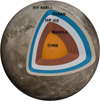 |
Fig. 1 Schematic illustration of an interior structure model of Ganymede, consisting of five concentric layers: an icy shell, a subsurface ocean, HP ice, a silicate mantle, and a fluid core. |
2.1 Love numbers
Juice will be able to measure both the vertical deformation, mainly due to Jupiter’s tidal potential, and the variations in the gravity field of Ganymede that arise due to the mass redistribution induced by the same tidal potential. These measurements will be possible thanks to the combined analysis of 3 GM radio tracking and the GALA altimeter (Van Hoolst et al. 2024). The response of a satellite to the external gravitational forcing by the primary planet is described by the solid-body tidal Love numbers h2, k2, and l2 of degree-two (Love 1909; Shida 1912). The Love numbers h2 and l2 describe the radial (ur) and lateral (u1) tidal displacements of the satellite, respectively. In particular,
![Mathematical equation: $\[u_{\mathrm{r}}=h_2 \frac{\mathcal{V}_2}{g} \text {, }\]$](/articles/aa/full_html/2025/07/aa54481-25/aa54481-25-eq2.png) (2)
(2)
where 𝒱2 is the degree-two time-dependent tidal potential and ![Mathematical equation: $\[g=G M_{\mathrm{G}} / R_{\mathrm{G}}^{2}\]$](/articles/aa/full_html/2025/07/aa54481-25/aa54481-25-eq3.png) is the surface gravitational acceleration, with MG and RG being Ganymede’s total mass and radius, respectively, and G the gravitational constant. Similarly, the k2 Love number describes the response of the body’s degree-two tidal potential caused by the internal displacements of mass. The incremental gravitational potential is given by
is the surface gravitational acceleration, with MG and RG being Ganymede’s total mass and radius, respectively, and G the gravitational constant. Similarly, the k2 Love number describes the response of the body’s degree-two tidal potential caused by the internal displacements of mass. The incremental gravitational potential is given by
![Mathematical equation: $\[\Delta \mathcal{V}=k_2 \mathcal{V}_2.\]$](/articles/aa/full_html/2025/07/aa54481-25/aa54481-25-eq4.png) (3)
(3)
In this work, we did not consider lateral surface variations, as the upcoming Juice data are expected to have limited sensitivity to the l2 Love number.
The Love numbers are bulk quantities that depend on the internal structure through the radial profiles of density, shear modulus, and viscosity (Moore & Schubert 2000). Since the viscoelastic properties of a body depend on the frequency of the external tidal forcing, the Love numbers are also frequency-dependent. Since, for the Galilean satellites, the main tidal cycle corresponds to their period of revolution, which for Ganymede is TG = 7.155 days, for the sake of simplicity we considered only the tidal forcing at the orbital frequency.
In general, the k2 and h2 Love numbers are complex numbers with amplitude and phase. The phase lags
![Mathematical equation: $\[\phi_{k_2}=\tan ^{-1} \frac{\operatorname{Im}\left(k_2\right)}{\operatorname{Re}\left(k_2\right)}, \quad \phi_{h_2}=\tan ^{-1} \frac{\operatorname{Im}\left(h_2\right)}{\operatorname{Re}\left(h_2\right)},\]$](/articles/aa/full_html/2025/07/aa54481-25/aa54481-25-eq5.png) (4)
(4)
contain information about the rheological and dissipative states of the satellites as they depend on the viscoelastic properties of the interior layers (Hussmann et al. 2016). For the special case of elastic planetary models, in which no dissipation due to friction occurs, the imaginary parts are equal to zero, and thus the respective phase lags vanish. With a slight abuse of notation, we sometimes refer to the real parts of the Love numbers as h2 and k2, respectively, when there is no risk of confusion. Jara-Orué & Vermeersen (2016) have found that the Love number k2 decreases with decreasing ocean density by about 23% for ocean densities in the range of 1000 kg m−3 to 1200 kg m−3, whereas h2 decreases by only 6%. The Love number k2 is therefore an excellent constraint on ocean density (Van Hoolst et al. 2024). The influence of uncertainties of the shell density (ρs) and rigidity (μs) in the values of the h2 and k2 Love numbers are less than 10% for realistic ranges of these parameters (Mitri et al. 2014; Jara-Orué & Vermeersen 2016), while the influence of the deeper interior on the Love numbers is below 1% (Jara-Orué & Vermeersen 2016; Kamata et al. 2016).
The Love numbers are also influenced by the viscosity of the ice shell, which can lead to large tidal deformations and dissipation. Dissipation is directly related to the phase lag, as it causes a delay in the tidal deformation relative to the tidal forcing. Unfortunately, viscosity is not well constrained and is strongly dependent on the thermal state (Moore & Schubert 2003; Van Hoolst et al. 2024). 3GM has the capability to determine the imaginary part of k2 with an accuracy of 6.8 × 10⁻⁵ (Cappuccio et al. 2020), thus providing key information on the ice shell viscosity and thermal state.
Except for a few special cases, closed-form analytical expressions for the Love numbers are not available, and they must be computed through numerical integration of the equilibrium equations or semi-analytical schemes. In this work, the frequency-dependent complex Love numbers h2 and k2 were computed using PyALMA3 (Petricca et al. 2024), a Python adaptation of the ALMA3 code (Melini et al. 2022). ALMA3 uses the viscoelastic normal modes method first introduced by Peltier (1974), which involves the propagation through the planetary layers of the fundamental solution of the equilibrium equations in the Laplace domain, and the solution of the secular equation whose roots determine the spectrum of viscoelastic relaxation times of the planetary body. Invoking the correspondence principle of linear viscoelasticity (Biot 1954; Fung 1965) the equilibrium equations can be cast in a formally elastic form by defining a complex rigidity μ(s) that depends on the adopted rheology and is a function of the Laplace variable, that is, the complex frequency s = iω. For a more detailed discussion, the reader is referred to Spada & Boschi (2006), Melini et al. (2022), and references therein. Throughout this work, the solid layers are modeled as Andrade viscoelastic shells. The Andrade rheological model, first introduced by Andrade (1910) to describe the stretching of metallic wires under constant stress, has become widely used in planetary science (see, e.g., Gevorgyan et al. 2020; Consorzi et al. 2024).
Compared to the simpler Maxwell model, the Andrade model is better suited for capturing high-frequency tidal deformations, making it particularly appropriate for Ganymede, given its short orbital period. The Andrade rheological law for the complex shear modulus reads
![Mathematical equation: $\[\mu(s)=\left[\frac{1}{\mu}+\frac{1}{\eta s}+\Gamma(\alpha+1) \frac{1}{\mu}\left(\frac{\eta s}{\mu}\right)^{-\alpha}\right]^{-1},\]$](/articles/aa/full_html/2025/07/aa54481-25/aa54481-25-eq6.png) (5)
(5)
where μ is the elastic shear modulus, η is the Newtonian viscosity, α is the creep parameter and Γ(x) is the Gamma function. Throughout this work, we assumed α = 1/3, the value originally proposed by Andrade (1910), although more recent studies allow α to take values between zero and unity (Walterová et al. 2023).
The fluid layers are modeled using the Newtonian rheology, and in this case, the complex rigidity is simply μ(s) = ηs. For the outer icy shell and HP ice layer, we adopted fixed rigidities of 3.3 and 6.6 GPa. The ice viscosity of the shell was sampled in the range 1013 to 1016 Pa s, while the viscosity of the HP ice layer was fixed at 1013 Pa s, a value compatible with a warm interior. For the silicate mantle, we used a rigidity of 50 GPa and a viscosity of 1020 Pa s. These values are consistent with those used in Hussmann et al. (2016). Lastly, both the ocean and the liquid iron core were treated as low-viscosity Newtonian fluids.
2.2 Libration amplitude of the icy shell
Due to Ganymede’s finite orbital eccentricity, Jupiter exerts a periodic torque on the triaxial figure of Ganymede. This, in turn, leads to physical librations (i.e., periodic variations in the rotation rate of the satellite) at the resonant orbital period. Besides the annual librations associated with a purely Keplerian motion, orbital perturbations, mainly due to interactions with the other Galilean satellites, the Sun, and Jupiter’s figure, give rise to librations with a wide spectrum of frequencies. However, although the amplitudes of the long-period librations may be large, they are almost independent of the interior structure (Rambaux et al. 2011). Furthermore, since the obliquity of Ganymede is expected to be small (Bills 2005), we restricted our attention to the longitudinal librations.
In the presence of a subsurface ocean, pressure, gravitational, viscous, and electromagnetic torques act to couple the ice shell to the ocean and the deeper interior (Van Hoolst et al. 2008, 2009). However, viscous torques acting at the ocean boundaries act over periods much longer than the annual libration period TG of just 7.155 days, and are thus ineffective at coupling the solid and liquid layers on such a short timescale (Baland & Van Hoolst 2010).
The analysis that we present next closely follows the formulation of Baland & Van Hoolst (2010), who have demonstrated that the libration amplitude at the orbital period (TG) depends primarily on the ice shell MoI (Cs), on the difference between the density of the ocean (ρo) and that of the outer shell (ρs), and only weakly on the deeper interior.
Let Aj < Bj < Cj be the principal Mols of the outer ellipsoidal surface of layer j. The z-component of the angular momentum equation for each layer can be written as
![Mathematical equation: $\[C_j \ddot{\phi}_j=\Gamma_j, \quad j \in \mathcal{I},\]$](/articles/aa/full_html/2025/07/aa54481-25/aa54481-25-eq7.png) (6)
(6)
where ϕj is the orientation angle between the long axis of layer j, which is associated with the smallest Mol (Aj) and a fixed direction in space, and Γj is the total torque acting on layer j due to gravitational interaction with Jupiter, internal gravitational forces between layers, and pressure forces on the boundaries between layers. Lastly, Cj is the polar MoI of layer j, which can be written as
![Mathematical equation: $\[C_j=\frac{8}{15} \pi \rho_j\left(R_j^5\left(1+\frac{2}{3} \alpha_j\right)-R_{j-1}^5\left(1+\frac{2}{3} \alpha_{j-1}\right)\right),\]$](/articles/aa/full_html/2025/07/aa54481-25/aa54481-25-eq8.png) (7)
(7)
where αj is the polar flattening of layer j, and Rj is its mean radius. The polar and equatorial flattening βj are defined as
![Mathematical equation: $\[\alpha_j=\frac{\left(a_j+b_j\right) / 2-c_j}{\left(a_j+b_j\right) / 2}, \quad \beta_j=\frac{a_j-b_j}{a_j},\]$](/articles/aa/full_html/2025/07/aa54481-25/aa54481-25-eq9.png) (8)
(8)
where aj > bj > cj are the lengths of the semi-axes of the outer ellipsoidal surface of layer j, with the longest axis pointing toward Jupiter. The polar and equatorial flattenings αs and βs are evaluated using the estimates of the triaxial figure from Burša (1997), which yield
![Mathematical equation: $\[\alpha_{\mathrm{s}}=4.301 \times 10^{-4}, \quad \beta_{\mathrm{s}}=5.154 \times 10^{-4}.\]$](/articles/aa/full_html/2025/07/aa54481-25/aa54481-25-eq10.png) (9)
(9)
For the sake of simplicity, in the following we assume that
![Mathematical equation: $\[\beta_{\mathrm{s}}=\beta_{\mathrm{o}}, \quad \alpha_{\mathrm{s}}=\alpha_{\mathrm{o}}, \quad \beta_j=\alpha_j=0, \quad j \neq \mathrm{s}, \mathrm{o}.\]$](/articles/aa/full_html/2025/07/aa54481-25/aa54481-25-eq11.png) (10)
(10)
By expanding Eq. (6) in terms of the mean anomaly (M) and eccentricity (e), Baland & Van Hoolst (2010) provide a solution that is correct up to the first order in terms of the small libration angles (γj = ϕj − M) and eccentricity (e). Solutions are sought of the form γj = gj sin M, where gj is the libration amplitude of layer j at the orbital period TG. Then, the libration amplitude of the outer shell can be written as
![Mathematical equation: $\[\begin{aligned}g_{\mathrm{s}} & \approx-6 e \frac{\left(B_{\mathrm{s}}-A_{\mathrm{s}}\right)+\left(B_{\mathrm{o}}-A_{\mathrm{o}}\right)}{C_{\mathrm{s}}} \\& \approx-6 e \frac{\left(\rho_{\mathrm{s}} \beta_{\mathrm{s}} R_{\mathrm{s}}^5+\left(\rho_{\mathrm{o}}-\rho_{\mathrm{s}}\right) \beta_{\mathrm{o}} R_{\mathrm{o}}^5\right)}{\rho_{\mathrm{s}}\left(R_{\mathrm{s}}^5\left(1+\frac{2}{3} \alpha_{\mathrm{s}}\right)-R_{\mathrm{o}}^5\left(1+\frac{2}{3} \alpha_{\mathrm{o}}\right)\right)},\end{aligned}\]$](/articles/aa/full_html/2025/07/aa54481-25/aa54481-25-eq12.png) (11)
(11)
where the equatorial MoI difference of layer j is expressed, correct up to first order in the equatorial flattening, as
![Mathematical equation: $\[B_j-A_j=\frac{8 \pi}{15} \int_{R_{j-1}}^{R_j} \rho_j \frac{\mathrm{~d}\left(\beta(r) r^5\right)}{\mathrm{d} r} \mathrm{~d} r, \quad j \in \mathcal{I}.\]$](/articles/aa/full_html/2025/07/aa54481-25/aa54481-25-eq13.png) (12)
(12)
Lastly, the libration amplitude of the outer shell at the equator can be written as Ls = |RGgs|. The main libration amplitude of the shell will be measured from GALA data, with an expected accuracy at the equator of about 10 m (Steinbrügge et al. 2019).
2.3 Moment of inertia
A direct constraint on the internal mass distribution is provided by the polar MoI, C, or equivalently by its nondimensional form, defined as ![Mathematical equation: $\[C_{\mathrm{nd}}=C /\left(M_{\mathrm{G}} R_{\mathrm{G}}^{2}\right)\]$](/articles/aa/full_html/2025/07/aa54481-25/aa54481-25-eq14.png) . For Ganymede, the gravity data acquired by the Galileo spacecraft during two close encounters with Ganymede led to a preliminary estimate of the moon’s gravity field quadrupole terms, under the assumption that Ganymede is in hydrostatic equilibrium, that is, J2 = (10/3) C22. These degree-2 gravity coefficients can be used to determine the mean Mol using the Darwin-Radau approximation (Murray & Dermott 1999). Using this approximation, Anderson et al. (1996) reported the value Cnd = 0.3105, the smallest among any planet or satellite in the Solar System. This value is significantly smaller than that of a spherical body of uniform density, for which Cnd = 2/5, and is thus an indication that the body’s mass is concentrated toward its center, suggesting a fully differentiated interior (Anderson et al. 1996). Nonetheless, it has been shown that the Darwin-Radau relation can lead to overestimating the Mol of Ganymede by more than 10%, when considering non-hydrostatic stresses at the surface or core-mantle boundary (Gao & Stevenson 2013).
. For Ganymede, the gravity data acquired by the Galileo spacecraft during two close encounters with Ganymede led to a preliminary estimate of the moon’s gravity field quadrupole terms, under the assumption that Ganymede is in hydrostatic equilibrium, that is, J2 = (10/3) C22. These degree-2 gravity coefficients can be used to determine the mean Mol using the Darwin-Radau approximation (Murray & Dermott 1999). Using this approximation, Anderson et al. (1996) reported the value Cnd = 0.3105, the smallest among any planet or satellite in the Solar System. This value is significantly smaller than that of a spherical body of uniform density, for which Cnd = 2/5, and is thus an indication that the body’s mass is concentrated toward its center, suggesting a fully differentiated interior (Anderson et al. 1996). Nonetheless, it has been shown that the Darwin-Radau relation can lead to overestimating the Mol of Ganymede by more than 10%, when considering non-hydrostatic stresses at the surface or core-mantle boundary (Gao & Stevenson 2013).
Under the assumption that all layers are spherical shells of uniform density ρj, with inner radius Rj−1 and outer radius Rj, the normalized polar MoI can be computed as
![Mathematical equation: $\[C_{\mathrm{nd}}=\frac{1}{M_{\mathrm{G}} R_{\mathrm{G}}^2} \sum_{j \in I} \frac{8}{15} \pi \rho_j\left(R_j^5-R_{j-1}^5\right), \quad R_0=0.\]$](/articles/aa/full_html/2025/07/aa54481-25/aa54481-25-eq15.png) (13)
(13)
This is equivalent to taking αj = 0 for all layers when evaluating Eq. (7).
2.4 Induced magnetic field
While ice is an insulator, the liquid water in the subsurface ocean is a conductive material. Whenever a conductive material is exposed to an external time-variable magnetic field, an induced magnetic field arises. In the case of the Galilean satellites, the induced fields are generated by temporal variations of Jupiter’s magnetic field at multiple frequencies. The orbit of Ganymede lies close to Jupiter’s equatorial plane, while the dipole axis of Jupiter’s strong magnetic field is tilted 9.6° with respect to its rotation axis (Acuna & Ness 1976). As a consequence, the magnetic field at the satellite’s location oscillates in time at Jupiter’s synodic period (TJ) of about 9.93 hours. Besides the main frequency, ω = 2π/TJ, other variations, not considered in this work, occur at fractions of the synodic period (e.g., TJ/2, TJ/3) due to higher-order harmonics of Jupiter’s internal field, at Ganymede’s orbital period, and at the solar rotation period (Seufert et al. 2011).
The electrical conductivity that determines the induction response of the water ocean is dependent on the salinity but also on the fluid’s temperature and pressure (Vance et al. 2021). However, results from Vance et al. (2021) show that the diffusive response for an ocean adiabatic conductivity profile and that of an ocean with uniform conductivity equal to the mean of the adiabatic profile differ by less than 1% (1.2 nT) and 2% (0.03 nT) at the synodic and orbital periods, respectively. Thus, for the sake of simplicity, we assumed the conductivity of the ocean to be uniform across the entire layer. Furthermore, we also assumed that the ocean is the only conductive layer. This assumption is justified by the fact that the conductivity of ice and silicates is negligible (Zimmer et al. 2000; Parkinson 1983), and although the conductivity of a molten iron core would be several orders of magnitude greater than that of the ocean, its induction signature is expected to be negligible due to attenuation of the signal as it propagates through the ocean (Vance et al. 2021; Petricca et al. 2023).
Inside the conducting ocean, the combination of Maxwell’s equations and Ohm’s law yields the diffusion equation for the magnetic field (Parkinson 1983; Zimmer et al. 2000), which reads
![Mathematical equation: $\[\nabla^2 \boldsymbol{B}=\mu_0 \sigma_{\mathrm{o}} \frac{\partial \boldsymbol{B}}{\partial t}.\]$](/articles/aa/full_html/2025/07/aa54481-25/aa54481-25-eq16.png) (14)
(14)
The solution of Eq. (14) can be decomposed as the sum of the primary Jovian field (Bext) and the induced field (Bind), that is, B = Bext + Bind. Moreover, the induced magnetic field of an arbitrary moon at time t can be related to that of a perfectly conducting moon (i.e., when σ → ∞) at time t − ϕA/ω, multiplied by the amplitude factor A, that is (Zimmer et al. 2000; Vance et al. 2021),
![Mathematical equation: $\[\boldsymbol{B}_{\mathrm{ind}}=A \boldsymbol{B}_{\mathrm{ind}, \infty}\left(t-\phi_A / \omega\right),\]$](/articles/aa/full_html/2025/07/aa54481-25/aa54481-25-eq17.png) (15)
(15)
where ϕA is the phase lag of the induced field. In the special case of a single, uniform conducting layer representing a saline ocean, we have (Vance et al. 2021; Srivastava 1966)
![Mathematical equation: $\[A \mathrm{e}^{-\mathrm{i} \phi_A}=\frac{j_{n+1}\left(k R_{\mathrm{o}}\right) y_{n+1}\left(k R_{\mathrm{i}}\right)-j_{n+1}\left(k R_{\mathrm{i}}\right) y_{n+1}\left(k R_{\mathrm{o}}\right)}{j_{n+1}\left(k R_{\mathrm{i}}\right) y_{n-1}\left(k R_{\mathrm{o}}\right)-j_{n-1}\left(k R_{\mathrm{o}}\right) y_{n+1}\left(k R_{\mathrm{i}}\right)},\]$](/articles/aa/full_html/2025/07/aa54481-25/aa54481-25-eq18.png) (16)
(16)
where jn and yn are the spherical Bessel functions of the first and second kind, respectively, of degree n, and ![Mathematical equation: $\[k=\sqrt{i \omega \mu_{0} \sigma_{0}}\]$](/articles/aa/full_html/2025/07/aa54481-25/aa54481-25-eq19.png) , with σ0 being the conductivity of the ocean layer and μ0 the magnetic permeability of free space.
, with σ0 being the conductivity of the ocean layer and μ0 the magnetic permeability of free space.
The fact that Ganymede possesses an intrinsic magnetic field does not alter the analysis. The intrinsic field can be assumed to be constant in time in a reference frame attached to Ganymede. For this reason, this field will appear only as a static offset to magnetometer measurements, similarly to the mean background field of Jupiter (Vance et al. 2021). The amplitude (A) and phase delay (ϕA) of the induced magnetic field, derived from Eq. (16), are treated as observables and used to impose additional constraints on Ganymede’s interior structure parameters.
3 Joint inversion: a machine learning approach
Synergies among different instruments on board Juice can be exploited to obtain a full picture of Ganymede’s interior structure. An analysis of the altimetric measurements from GALA in combination with precise orbit reconstruction from 3GM data will provide estimates of the h2 Love number. The altimetric profiles, in combination with stereo digital terrain models derived from JANUS images, will also yield estimates of the libration amplitude of the icy shell. The data acquired during the Ganymede circular orbit phase by the magnetometer J-MAG will be used to measure the induced magnetic field response of Ganymede at multiple frequencies, while the radio science experiment 3GM will provide estimates of the complex Love number k2 and gravitational field of Ganymede. The latter will also enable refined estimates of the Mol of Ganymede by assessing the deviation from the hydrostatic equilibrium ratio. However, the severe differences in the analysis tools and kinds of data captured by the different instruments on board Juice, make a joint inversion of all data simultaneously a very challenging task (Van Hoolst et al. 2024). One possible strategy for performing the inversion is to employ a Markov chain Monte Carlo method (for an overview, see Sambridge & Mosegaard 2002).
We propose, as an alternative method for finding solutions to the inverse problem, the use of a neural network to recognize the intricate relationships between a set of observable parameters and the underlying internal structure model. The main advantage over a more traditional Markov chain Monte Carlo approach is that the forward modeling, required to build the synthetic dataset, needs to be done just once, before training (Käufl et al. 2016; Agarwal et al. 2021).
With this goal in mind, we trained a neural network on a synthetic dataset of plausible interior structures of Ganymede; for each structure we computed a set of observable parameters using analytical and numerical models from the literature, as described in Sect. 2. The input layer of the neural network consists of the parameter vector of the observables
![Mathematical equation: $\[\boldsymbol{x}=\left(\operatorname{Re}\left(h_2\right), \phi_{h_2}, \operatorname{Re}\left(k_2\right), \phi_{k_2}, A, \phi_A, C_{\mathrm{nd}}, L_{\mathrm{s}}\right).\]$](/articles/aa/full_html/2025/07/aa54481-25/aa54481-25-eq20.png) (17)
(17)
On the other hand, the output layer is constituted by the thicknesses and densities of each layer, the viscosity of the shell, and the ocean conductivity, that is,
![Mathematical equation: $\[\boldsymbol{y}=\left(d_{\mathrm{s}}, \rho_{\mathrm{s}}, \eta_{\mathrm{s}}, d_{\mathrm{o}}, \rho_{\mathrm{o}}, \sigma_{\mathrm{o}}, d_{\mathrm{i}}, \rho_{\mathrm{i}}, d_{\mathrm{m}}, \rho_{\mathrm{m}}, d_{\mathrm{c}}, \rho_{\mathrm{c}}\right).\]$](/articles/aa/full_html/2025/07/aa54481-25/aa54481-25-eq21.png) (18)
(18)
A sketch of the neural network structure is shown in Fig. 2.
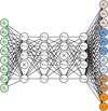 |
Fig. 2 Schematic representation of the neural network used in this work. On the left we have the input layer with the observable parameters (x), in the middle the four hidden layers, and on the right the output layer constituted by the internal structure parameters (y). A black cross indicates nodes that have been disabled by the dropout layers. |
4 Synthetic icy satellites dataset
We generated a synthetic dataset of N = 107 icy satellites by performing a Monte Carlo sampling of the internal structure parameters compatible with Ganymede’s mean radius (RG) and mass (MG), as reported in Table 1. The thicknesses (dj) of each layer are uniformly sampled in the respective ranges shown in Table 2, except for the mantle thickness (dm) that is chosen in order to satisfy the total radius (RG) constraint.
The upper limits for the thicknesses of the icy shell and ocean ds and do were both set at RG/10 = 263.1 km, the maximum thickness for the HP ice layer (di) is 3RG/10 = 789.3 km, while the core thickness (dc) ranged from a minimum of RG/10 to a maximum of RG/2 = 1315.6 km. The outer radius of the i-th layer is related to its thickness by
![Mathematical equation: $\[R_j=R_{j-1}+d_j, \quad j \in \mathcal{I}, \quad R_0=0.\]$](/articles/aa/full_html/2025/07/aa54481-25/aa54481-25-eq22.png) (19)
(19)
The next step was to sample the densities (ρj) for each internal layer. Densities were sampled sequentially from the outermost to the innermost layer, except for the silicate mantle density (ρm), which was chosen to satisfy the total mass (MG) constraint. The densities of the outer shell (ρs) and ocean (ρo) have an upper limit of 1200 kg m−3, while that of the HP ice (ρi) is 1400 kg m−3, following Baland & Van Hoolst (2010). The lower limit for the outer shell density is set at 800 kg m−3, while the lower limits for the ocean and HP ice densities are not fixed, but depend on the density of the layer directly above it, in order to enforce the constraint ρj ≤ ρj−1, ensuring that density does not decrease with depth. For the mantle, we consider a broad range of densities (ρm), from 2500 kg m−3 to a maximum of 5000 kg m−3. This choice is conservative, as previous studies usually adopt narrower density intervals for the silicate mantle (see, e.g., Sohl et al. 2002; Baland & Van Hoolst 2010). Lastly the core density (ρc) is allowed to vary between 5000 kg m−3 and 8000 kg m−3, roughly corresponding to a eutectic Fe − FeS composition and pure iron core, respectively (Anderson et al. 1996; Sohl et al. 2002). The mass (mj) of each of these layers was computed using the sampled thickness (dj) and density (ρj) in the approximation of spherical layers of outer radius Rj and inner radius Rj−1, that is,
![Mathematical equation: $\[m_j=\frac{4}{3} \pi \rho_j\left(R_j^3-R_{j-1}^3\right), \quad j \in \mathcal{I}.\]$](/articles/aa/full_html/2025/07/aa54481-25/aa54481-25-eq23.png) (20)
(20)
Then, the density of the silicate mantle (ρm) can be easily determined using the constraint on the total mass of Ganymede (MG). If the resulting density of the mantle falls outside the bounds defined above, the sample is discarded and a new one is drawn from scratch. The ocean conductivity (σo) and the viscosity of the ice shell (ηs) are uniformly sampled within the ranges given in Table 2.
Once all the internal structure parameters are sampled, we proceeded to compute the corresponding values of the complex Love numbers h2 and k2 at the orbital period of Ganymede using PyALMA3. Then we computed the libration amplitude of the icy shell (Ls), as described in Sect. 2.2, and the amplitude (A) and phase lag (ϕA) of the induced magnetic field at Jupiter’s synodic rotation period using Eq. (16). Lastly, we computed the normalized polar MoI for the whole of Ganymede using Eq. (13).
We then filtered the dataset to retain only interior structures that satisfy h2 > 1.0 and k2 > 0.25, effectively removing models that correspond to nearly degenerate cases with vanishing ocean thickness (do). We also filtered out models that result in libration amplitudes larger than 4.6 km, the upper limit provided by Zubarev et al. (2015). Also, these latter models all correspond to unrealistically thin icy shells. In Fig. A.1 we show the distributions of the interior structure parameters (y) and the corresponding observables, x = x(y), that constitute the synthetic dataset.
Physical parameters of Ganymede.
Values of the interior structure parameters of Ganymede used in this study.
5 Neural network architecture
At its essence, the neural network is a function,
![Mathematical equation: $\[f(\boldsymbol{x}; \boldsymbol{w})=\boldsymbol{y},\]$](/articles/aa/full_html/2025/07/aa54481-25/aa54481-25-eq24.png) (21)
(21)
that maps the input observables (x) into the output parameters (y), and w = (w1,1, . . ., wl,m) is a set of weights that parametrize the mapping. The values of the weights are iteratively adjusted during the training process to minimize a loss function, thereby enabling the network to approximate the underlying relationship between inputs and outputs.
For our neural network, we used l = 4 dense hidden layers with m = 128 nodes each. The hidden layers are activated with a rectified linear unit (ReLU), that is,
![Mathematical equation: $\[\operatorname{ReLU}(x)=\max (0, x).\]$](/articles/aa/full_html/2025/07/aa54481-25/aa54481-25-eq25.png) (22)
(22)
Being a piecewise linear function, the ReLU is easy to optimize and retains many of the advantages of linear models (Goodfellow et al. 2016), making it a common choice among nonlinear activation functions. For the output layer, a linear activation function is used.
We included a dropout layer after each hidden layer, with a dropout rate of pd = 0.02 (Srivastava et al. 2014). At each training epoch, the dropout layer randomly disables a fraction of the nodes specified by the parameter pd (i.e., 2% in this case). The role of the dropout layer is twofold: (i) it helps prevent overfitting, and (ii) it allows us to estimate the model prediction uncertainties by running multiple predictions with the dropout layers active at the inference stage (Gal & Ghahramani 2016). In Fig. 2 we show a schematic representation of the neural network architecture used in this work.
Before training, both the input and output parameters are standardized, meaning each feature’s distribution is transformed to have zero mean and unit variance. This preprocessing step improves the convergence speed and training stability of the neural network. The loss function used to train the model is the mean squared error, a common choice for regression problems.
It would be desirable that the predicted output parameters of the neural network satisfy the constraints imposed by the mass and radius, that is,
![Mathematical equation: $\[\sum_{j \in I} d_j=R_{\mathrm{G}}, \quad \sum_{j \in I} m_j=M_{\mathrm{G}}.\]$](/articles/aa/full_html/2025/07/aa54481-25/aa54481-25-eq26.png) (23)
(23)
To this aim, we considered using a custom loss function that penalizes output thicknesses that add up to values different from the total radius, and densities that do not comply with the total mass constraint. However, we noticed that this is less important than using the standard scaler for both input and output features.
The minimization of the loss function was performed using the AdamW optimizer (Loshchilov & Hutter 2017), which modifies the popular Adam optimizer (Kingma & Ba 2014) by decoupling the weight decay from the gradient update, in practice leading to improved generalization performance. We also used a variable learning rate, decreasing it whenever the loss function stagnates for several consecutive epochs. The learning rate determines how much the neural network weights are allowed to change at each update during the optimization process. To prevent any issues with the model overfitting the training data, we adopted early stopping (Prechelt 1998) and stopped the training once the minimum prescribed learning rate was reached and the loss metric from the validation data did not significantly improve for a given number of consecutive training epochs.
The dataset was split into training and validation sets. The training set contains 80% of the data and the validation set the remaining 20%, which is not seen by the model during training. The neural network is trained using the Keras deep learning API (Chollet 2017), which is built on top of the Python-based and open source TensorFlow platform (Abadi et al. 2016).
It is worth noting that typical dropout rates found in the literature are usually higher than the one used here. Furthermore, it has been demonstrated that its value can have a significant impact on the model uncertainty (see, e.g., Verdoja & Kyrki 2020). The dropout rate (pd) and number of nodes (m) used in this work were selected after performing a grid search. We find that m has a limited impact on performance, though the general trend suggests that reducing the number of nodes leads to a slightly higher validation loss. On the other hand, the dropout rate requires careful tuning: we observe that only the smaller values enhance generalization by preventing overfitting, whereas higher values negatively impact the ability of our model to make reliable predictions.
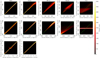 |
Fig. 3 Comparison of the actual values of the interior structure parameters (y) with those predicted by the neural network for the validation dataset |
![Mathematical equation: $\[(\hat{\boldsymbol{y}})\]$](/articles/aa/full_html/2025/07/aa54481-25/aa54481-25-eq27.png)
6 Inference uncertainty
To capture the uncertainty in the predicted parameters, which is intrinsic to this inverse problem, it is desirable to obtain a posterior distribution of the interior structure parameters, rather than deterministic values. To do this, we used the Monte Carlo dropout approach (Gal & Ghahramani 2016), which allows us to obtain an approximate Bayesian inference through dropout training. The rough idea is that by leaving the dropout layers active during the inference, it is possible to run multiple predictions starting from the same set of observables (x), leading to slightly different output parameters ![Mathematical equation: $\[(\hat{\boldsymbol{y}})\]$](/articles/aa/full_html/2025/07/aa54481-25/aa54481-25-eq28.png) each time. The set of these predictions constitutes a discrete distribution of plausible interior structure parameters compatible with the input parameters (x).
each time. The set of these predictions constitutes a discrete distribution of plausible interior structure parameters compatible with the input parameters (x).
To obtain a more robust estimate of the predicted interior structures’ distribution, we also need to account for possible errors in the input parameters (x) to ensure that small deviations in x do not yield significantly different values for ![Mathematical equation: $\[\hat{\boldsymbol{y}}\]$](/articles/aa/full_html/2025/07/aa54481-25/aa54481-25-eq29.png) . To this end, during inference, before each prediction, we also modified the input parameters by adding white noise to the input features. For all features, the white noise has zero mean and standard deviation corresponding to 1% of the corresponding input feature value (i.e., σ(x) = 0.01 x). This is a conservative choice, since the expected accuracy of the h2 measurement from GALA are smaller than 2% (Steinbrügge et al. 2015), while for k2 the expected accuracy that will be achieved with 3 GM is of σ(k2) ~ 10−4 (Cappuccio et al. 2020). For the ocean conductivity, we expect an error on the order of 2% to be introduced by the uniform conductivity assumption (Vance et al. 2021), as already noted.
. To this end, during inference, before each prediction, we also modified the input parameters by adding white noise to the input features. For all features, the white noise has zero mean and standard deviation corresponding to 1% of the corresponding input feature value (i.e., σ(x) = 0.01 x). This is a conservative choice, since the expected accuracy of the h2 measurement from GALA are smaller than 2% (Steinbrügge et al. 2015), while for k2 the expected accuracy that will be achieved with 3 GM is of σ(k2) ~ 10−4 (Cappuccio et al. 2020). For the ocean conductivity, we expect an error on the order of 2% to be introduced by the uniform conductivity assumption (Vance et al. 2021), as already noted.
7 Results and discussion
The trained model demonstrates significant predictive accuracy in estimating the thickness and density distributions of candidate interior structures of Ganymede with varying levels of accuracy across different layers. In Fig. 3, we show a comparison between the actual values of the interior parameters y and those predicted by our trained neural network for the validation dataset ![Mathematical equation: $\[\hat{\boldsymbol{y}}\]$](/articles/aa/full_html/2025/07/aa54481-25/aa54481-25-eq30.png) . A perfect prediction for an interior structure parameter y ∈ y would fall on the
. A perfect prediction for an interior structure parameter y ∈ y would fall on the ![Mathematical equation: $\[y=\hat{y}\]$](/articles/aa/full_html/2025/07/aa54481-25/aa54481-25-eq31.png) line.
line.
To quantify the accuracy of the model, we computed the mean absolute error (MAE) of the predicted parameters with respect to the actual values. The MAE is defined as
![Mathematical equation: $\[\operatorname{MAE}(y)=\frac{1}{N_{\mathrm{v}}} \sum_{n=1}^{N_{\mathrm{v}}}\left|y_n-\hat{y}_n\right|, \quad y \in \boldsymbol{y},\]$](/articles/aa/full_html/2025/07/aa54481-25/aa54481-25-eq32.png) (24)
(24)
where Nv ≈ 2 × 10⁶ is the number of samples in the validation dataset, and yn and ![Mathematical equation: $\[\hat{y}_n\\]$](/articles/aa/full_html/2025/07/aa54481-25/aa54481-25-eq33.png) denote a particular sample from the validation dataset, and one prediction made by the neural network, respectively.
denote a particular sample from the validation dataset, and one prediction made by the neural network, respectively.
It is worth noting that in the computation of the MAEs, no white noise was added to the input parameter vector (x), and we only considered a single prediction, ![Mathematical equation: $\[\hat{\boldsymbol{y}}\]$](/articles/aa/full_html/2025/07/aa54481-25/aa54481-25-eq36.png) , made by the neural network from the input (x). We find that the trained neural network is able to capture the thickness ds and density ρs of the icy shell with excellent accuracy with MAEs of just 2.8 km and 11.5 kg m−3, respectively, as well as the ice viscosity (ηs) with MAEs of 0.05 log10Pa s.
, made by the neural network from the input (x). We find that the trained neural network is able to capture the thickness ds and density ρs of the icy shell with excellent accuracy with MAEs of just 2.8 km and 11.5 kg m−3, respectively, as well as the ice viscosity (ηs) with MAEs of 0.05 log10Pa s.
Very good agreement between the predicted and actual values is found also for the ocean thickness (do) and density (ρo) with MAEs of just 9.5 km and 6.0 kg m−3, respectively, and also for the conductivity (σo), for which the MAE is of 0.1 S m−1. The model is also able to predict the thickness and density of the HP ice layer di with reasonable accuracy, with MAEs of 39.8 km and 18.8 kg m−3, respectively.
The model performs poorly in the task of inferring the thickness and density of the core and mantle, suggesting limited sensitivity of the selected observables to these parameters. However, this had to be expected, and is in line with previous results present in the literature, indicating that the Love numbers are not useful in constraining the properties of the deeper layers of Ganymede (Wahr et al. 2006; Kamata et al. 2016) and Europa (Petricca et al. 2024). Notably in the case of the core density ρc, the model consistently predicts values close to the mean of the training dataset (i.e., approximately 6500 kg m−3).
This behavior is related to the low sensitivity of the observable parameters (x) to variations in ρc, which leads to a broad set of equally viable solutions. As a result, minimizing the mean squared error during training encourages predictions to converge toward the mean of the target distribution, as this effectively minimizes the loss function (see, e.g., Bishop 1994).
Ideally, the predicted interior structure models described by the parameter set ![Mathematical equation: $\[\hat{\boldsymbol{y}}\]$](/articles/aa/full_html/2025/07/aa54481-25/aa54481-25-eq37.png) should be consistent with the input parameters (x) used to generate the prediction. In Fig. 4 we compare the x observables that correspond to the interior structure parameters (y) from the validation dataset with
should be consistent with the input parameters (x) used to generate the prediction. In Fig. 4 we compare the x observables that correspond to the interior structure parameters (y) from the validation dataset with ![Mathematical equation: $\[\hat{\boldsymbol{x}}\]$](/articles/aa/full_html/2025/07/aa54481-25/aa54481-25-eq38.png) , the set of observables that we computed starting from one noise-free, single-shot prediction from the neural network
, the set of observables that we computed starting from one noise-free, single-shot prediction from the neural network ![Mathematical equation: $\[\hat{\boldsymbol{y}}\]$](/articles/aa/full_html/2025/07/aa54481-25/aa54481-25-eq39.png) . To quantify the agreement, we computed the MAE, defined in analogy with Eq. (24), between the actual input parameters x and
. To quantify the agreement, we computed the MAE, defined in analogy with Eq. (24), between the actual input parameters x and ![Mathematical equation: $\[\hat{\boldsymbol{x}}\]$](/articles/aa/full_html/2025/07/aa54481-25/aa54481-25-eq40.png) . We find that the MAE is less than 6 × 10⁻³ for the Love numbers Re(h2) and Re(k2), and less than 0.2° for the phase lags ϕh2 and ϕk2. For the amplitude of the induced magnetic field A, the MAE is 5 × 10⁻³, while for its associated phase lag, ϕA, the MAE is 0.7°. The MAE for the polar MoI (Cnd) is on the order of 10−3, while for the libration amplitude (Ls), the MAE is about 20 m, only slightly larger than the expected libration measurement accuracy of GALA (Steinbrügge et al. 2019).
. We find that the MAE is less than 6 × 10⁻³ for the Love numbers Re(h2) and Re(k2), and less than 0.2° for the phase lags ϕh2 and ϕk2. For the amplitude of the induced magnetic field A, the MAE is 5 × 10⁻³, while for its associated phase lag, ϕA, the MAE is 0.7°. The MAE for the polar MoI (Cnd) is on the order of 10−3, while for the libration amplitude (Ls), the MAE is about 20 m, only slightly larger than the expected libration measurement accuracy of GALA (Steinbrügge et al. 2019).
We also note that the interior structure parameters ![Mathematical equation: $\[\hat{\boldsymbol{y}}\]$](/articles/aa/full_html/2025/07/aa54481-25/aa54481-25-eq41.png) , predicted by the neural network from the observables in the validation dataset, satisfy the mass and radius constraints of Eq. (23) with mean relative errors of 5 × 10⁻³ and 4 × 10⁻⁴, respectively, even though these constraints were not explicitly imposed in the loss function, but were implicitly contained in the training data. This shows that even though the density and thickness of the core and mantle are not well constrained, the neural network is still able to predict values that are consistent with the total mass and radius of Ganymede.
, predicted by the neural network from the observables in the validation dataset, satisfy the mass and radius constraints of Eq. (23) with mean relative errors of 5 × 10⁻³ and 4 × 10⁻⁴, respectively, even though these constraints were not explicitly imposed in the loss function, but were implicitly contained in the training data. This shows that even though the density and thickness of the core and mantle are not well constrained, the neural network is still able to predict values that are consistent with the total mass and radius of Ganymede.
By inspecting the distribution of the predicted parameters of Fig. 3, we find that the neural network tends to overestimate values near the inferior limit of the distribution, that is, ![Mathematical equation: $\[\hat{y}>y\]$](/articles/aa/full_html/2025/07/aa54481-25/aa54481-25-eq42.png) , and vice versa it underestimates those closer to the upper limit, that is,
, and vice versa it underestimates those closer to the upper limit, that is, ![Mathematical equation: $\[\hat{y}<y\]$](/articles/aa/full_html/2025/07/aa54481-25/aa54481-25-eq43.png) . These effects are more severe for those parameters whose underlying distribution in the synthetic dataset presents a tail-like shape toward the lower and upper limits, respectively, as can be seen in Fig. A.1.
. These effects are more severe for those parameters whose underlying distribution in the synthetic dataset presents a tail-like shape toward the lower and upper limits, respectively, as can be seen in Fig. A.1.
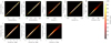 |
Fig. 4 Comparison of the actual observables (x) in the validation dataset with the corresponding observables ( |
![Mathematical equation: $\[\hat{\boldsymbol{x}}\]$](/articles/aa/full_html/2025/07/aa54481-25/aa54481-25-eq34.png)
![Mathematical equation: $\[(\hat{\boldsymbol{y}})\]$](/articles/aa/full_html/2025/07/aa54481-25/aa54481-25-eq35.png)
7.1 Example: posterior distributions for selected observables
As an example, in Fig. 5 we show the posterior distributions of the internal structure parameters ![Mathematical equation: $\[(\hat{\boldsymbol{y}})\]$](/articles/aa/full_html/2025/07/aa54481-25/aa54481-25-eq44.png) that correspond to the set of observables (x*), shown in Table 3, which was randomly selected from the validation dataset. The distribution is obtained using a dropout rate of pd = 0.02, the same used during training, and repeating the predictions Np = 104 times. Before each of the Np predictions, we also added white noise to the input features as described in Sect. 6.
that correspond to the set of observables (x*), shown in Table 3, which was randomly selected from the validation dataset. The distribution is obtained using a dropout rate of pd = 0.02, the same used during training, and repeating the predictions Np = 104 times. Before each of the Np predictions, we also added white noise to the input features as described in Sect. 6.
We observe that the true values of the internal structure parameters y* fall within the posterior distributions, close to the mean values ![Mathematical equation: $\[\mu(\hat{\boldsymbol{y}})\]$](/articles/aa/full_html/2025/07/aa54481-25/aa54481-25-eq47.png) , in the case of the icy shell, the ocean, and HP ice layer. The predictions of the parameters associated with the deeper layers are less reliable as they are not well constrained by the observables used in this work, as previously noted.
, in the case of the icy shell, the ocean, and HP ice layer. The predictions of the parameters associated with the deeper layers are less reliable as they are not well constrained by the observables used in this work, as previously noted.
The Monte Carlo dropout method operates by modifying the mapping in Eq. (21), deactivating a randomly selected subset of the neurons during inference, resulting in a perturbed mapping for each forward pass. In principle, this allows the model to sample diverse solutions. However, the resulting predictions may still be concentrated in a narrow region of the solution space, failing to fully represent the broader set of solution and correctly assess uncertainty (Fort et al. 2020).
To test this behavior, we took the set of interior structures ![Mathematical equation: $\[(\hat{\boldsymbol{y}})\]$](/articles/aa/full_html/2025/07/aa54481-25/aa54481-25-eq48.png) , which was obtained starting from the set of observables x* (see Fig. 5), and replaced the mantle and core density thickness with newly sampled values, subject to the same constraints that were used to generate the synthetic dataset (see Sect. 4). We denote this new distribution
, which was obtained starting from the set of observables x* (see Fig. 5), and replaced the mantle and core density thickness with newly sampled values, subject to the same constraints that were used to generate the synthetic dataset (see Sect. 4). We denote this new distribution ![Mathematical equation: $\[\hat{\boldsymbol{y}}_{\text {new}}\]$](/articles/aa/full_html/2025/07/aa54481-25/aa54481-25-eq49.png) . Then, we selected only the interior structures within
. Then, we selected only the interior structures within ![Mathematical equation: $\[\hat{\boldsymbol{y}}_{\text {new}}\]$](/articles/aa/full_html/2025/07/aa54481-25/aa54481-25-eq50.png) whose observables fall reasonably close to x*. More precisely, we define
whose observables fall reasonably close to x*. More precisely, we define
![Mathematical equation: $\[\hat{\boldsymbol{y}}_{\text {match }}=\left\{\boldsymbol{y} \in \hat{\boldsymbol{y}}_{\text {new }} \mid \boldsymbol{x}(\boldsymbol{y}) \in\left\{\boldsymbol{x}^* \pm 3 \sigma\left(\boldsymbol{x}^*\right)\right\}\right\},\]$](/articles/aa/full_html/2025/07/aa54481-25/aa54481-25-eq51.png) (25)
(25)
where the standard deviation, σ(x*), is defined as in Sect. 6.
Within the distribution ![Mathematical equation: $\[\hat{\boldsymbol{y}}_{\text {match}}\]$](/articles/aa/full_html/2025/07/aa54481-25/aa54481-25-eq52.png) , we find candidate internal structures with core densities ρc covering the entire samples space (see Table 2), in sharp contrast with the predictions from the neural network that is only able to detect solutions with a core density close to the mean of the dataset. Since the constraints of Eq. (23) are enforced on
, we find candidate internal structures with core densities ρc covering the entire samples space (see Table 2), in sharp contrast with the predictions from the neural network that is only able to detect solutions with a core density close to the mean of the dataset. Since the constraints of Eq. (23) are enforced on ![Mathematical equation: $\[\hat{\boldsymbol{y}}_{\text {match}}\]$](/articles/aa/full_html/2025/07/aa54481-25/aa54481-25-eq53.png) , and are satisfied in an approximate way also by the neural network predictions
, and are satisfied in an approximate way also by the neural network predictions ![Mathematical equation: $\[\hat{\boldsymbol{y}}\]$](/articles/aa/full_html/2025/07/aa54481-25/aa54481-25-eq54.png) , we expect the variability in core density ρc to be accompanied by variability in core thickness dc to preserve the total mass MG, and consequently in mantle thickness dm to comply with the total radius RG. We find plausible interior structures within
, we expect the variability in core density ρc to be accompanied by variability in core thickness dc to preserve the total mass MG, and consequently in mantle thickness dm to comply with the total radius RG. We find plausible interior structures within ![Mathematical equation: $\[\hat{\boldsymbol{y}}_{\text {match}}\]$](/articles/aa/full_html/2025/07/aa54481-25/aa54481-25-eq55.png) with core thicknesses (dc) that cover all possible values up to approximately 850 km, while the predicted values,
with core thicknesses (dc) that cover all possible values up to approximately 850 km, while the predicted values, ![Mathematical equation: $\[\hat{d}_{\mathrm{c}}\]$](/articles/aa/full_html/2025/07/aa54481-25/aa54481-25-eq56.png) , lie in a smaller range of roughly 400 km to 550 km. Accordingly, we find that the mantle thickness (dm) can range approximately from 1250 km to 2100 km, while the predicted values
, lie in a smaller range of roughly 400 km to 550 km. Accordingly, we find that the mantle thickness (dm) can range approximately from 1250 km to 2100 km, while the predicted values ![Mathematical equation: $\[(\hat{d}_{\mathrm{m}})\]$](/articles/aa/full_html/2025/07/aa54481-25/aa54481-25-eq57.png) vary in a narrower range, from about 1500 km to 1750 km. On the other hand we do not observe any significant change in the distribution of the mantle density predicted by the neural network (
vary in a narrower range, from about 1500 km to 1750 km. On the other hand we do not observe any significant change in the distribution of the mantle density predicted by the neural network (![Mathematical equation: $\[\hat{\rho}_{\mathrm{m}}\]$](/articles/aa/full_html/2025/07/aa54481-25/aa54481-25-eq58.png) ) and those present in the distribution
) and those present in the distribution ![Mathematical equation: $\[\hat{\boldsymbol{y}}_{\text {match}}\]$](/articles/aa/full_html/2025/07/aa54481-25/aa54481-25-eq59.png) . This last result is in agreement with Fig. 3, which shows that ρm is well constrained by the neural network, at least in the lower part of the sample space, as is the case for the distribution
. This last result is in agreement with Fig. 3, which shows that ρm is well constrained by the neural network, at least in the lower part of the sample space, as is the case for the distribution ![Mathematical equation: $\[\hat{\boldsymbol{y}}\]$](/articles/aa/full_html/2025/07/aa54481-25/aa54481-25-eq60.png) (see Fig. 5).
(see Fig. 5).
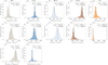 |
Fig. 5 Histograms of the distribution of the interior structure parameters |
![Mathematical equation: $\[(\hat{\boldsymbol{y}})\]$](/articles/aa/full_html/2025/07/aa54481-25/aa54481-25-eq45.png)
![Mathematical equation: $\[\mu(\hat{\boldsymbol{y}})\]$](/articles/aa/full_html/2025/07/aa54481-25/aa54481-25-eq46.png)
Values of the representative set of parameters (x*) drawn from the validation dataset.
7.2 Toward a more realistic model
It must be noted that the interior structure model presented in this work is relatively simple. Future research should aim to incorporate a more realistic description of Ganymede’s interior (see, e.g., Hussmann et al. 2010), as well as additional constraints on the interior structure from measurements of Ganymede’s obliquity, global shape, gravity, and intrinsic magnetic field (see, e.g., Van Hoolst et al. 2024). In particular, a more sophisticated model should account for pressure-induced phase transitions within the hydrosphere (see Sohl et al. 2002; Spohn & Schubert 2003). Additionally, the impact of variable rigidities and viscosities on the Love numbers warrants further investigation, particularly for the HP ice layer, where viscosity strongly depends on temperature and can largely influence tidal deformation and dissipation. Indeed, as Petricca et al. (2024) demonstrated, the shear modulus of the ice layers can significantly bias the inferred ice thickness, in agreement with the earlier findings of Moore & Schubert (2000) and Wahr et al. (2006), showing that tidal amplitudes vary linearly with the ice thickness, with the slope of the relationship controlled by the ice rigidity.
8 Conclusions
We trained a neural network to recognize interior structure parameters of Ganymede, namely the thicknesses (dj) and densities (ρj) of each of the five layers, as well as the viscosity of the icy shell (ηs) and the conductivity of the subsurface ocean (σo). The neural network was trained using a synthetic dataset of possible interior structure parameters that we generated via Monte Carlo sampling, with additional constraints to satisfy the total mass and radius of Ganymede.
For each interior structure, we computed a set of parameters, namely: the normalized polar MoI; the h2 and k2 Love numbers and their associated phase lags (ϕh2 and ϕk2) using PyALMA3 (Petricca et al. 2024; Melini et al. 2022); the normalized amplitude (A) and phase (ϕA) of the induced magnetic field at the orbital period from the model of Vance et al. (2021), and the longitudinal libration amplitude at the equator (Ls) using models from Baland & Van Hoolst (2010).
The trained model accurately estimated the thickness and density distributions of Ganymede-like icy satellites, with varying levels of accuracy across different layers. The neural network was able to capture the thickness and density of the icy shell and ocean with excellent accuracy. The model also showed reasonable accuracy in predicting the thickness and density of the HP ice layer. However, it struggled to constrain the deeper interior, performing poorly in inferring the thickness and density of the core and mantle, which suggests a limited sensitivity of the chosen features to the internal structure parameters.
The Monte Carlo dropout method in combination with the addition of noise to the input parameters, to simulate measurement and modeling errors, was used to assess the robustness of the predicted parameters, providing a posterior distribution of the interior structure parameters. The true values of the parameters fell within the posterior distributions, close to their respective mean values, except for the core and mantle thickness and density, which are not well constrained by the observables used in this work.
Furthermore, we have shown that the methodology presented here falls short in assessing the uncertainty in the deeper interior since the intrinsic degeneracy in the inverse problem allows for a broader range of deep interior structures than those predicted by the neural network. This limitation of the Monte Carlo dropout method has already been pointed out in the literature (see, e.g., Fort et al. 2020).
Nevertheless, this work demonstrates the potential of machine learning to complement traditional modeling approaches, providing a fast and preliminary tool for identifying families of interior structures compatible with synthetic observables or, in the future, with data provided by the Juice mission following its arrival at Ganymede in the coming decade.
Acknowledgements
G.M. acknowledges support from the Italian National Recovery and Resilience Plan (PNRR), funded by the European Union under the NextGenerationEU initiative (CUP: C96E23000680001). G.M. thanks Leonardo Pagliaro and Lorenzo Spina for their insightful suggestions, especially during the early stages of this work, and Daniele Melini for his assistance with the ALMA3 code. G.M. also gratefully acknowledges the fruitful discussions with colleagues met in Pescara at the XX Congresso Nazionale di Scienze Planetarie, and at the DLR Institute of Planetary Research in Berlin. We are also indebted to Hauke Hussmann for his valuable comments and feedback. Last but not least, we thank the anonymous referee for their constructive comments and suggestions, which have significantly improved the final version of this work.
Appendix A Distributions of input and output parameters
In Fig. A.1 we present histograms of the distributions of the observable parameters (x) in the synthetic dataset. These include the normalized polar MoI (Cnd), the real parts of the radial and gravitational tidal Love numbers (h2 and k2), their respective phase lags (ϕh2 and ϕk2), the amplitude (A) and phase lag (ϕA) of the induced magnetic field at the synodic period of Jupiter (TJ), and the longitudinal libration amplitude (LS) at Ganymede’s orbital period (TG). The ranges for Re(h2) and Re(k2) are compatible with those of Ganymede interior models with a subsurface ocean of previous studies (e.g., Kamata et al. 2016). In Fig. A.1 we also show the distributions of the underlying interior structure parameters y, that is, the thicknesses (dj) and densities (ρj) of the layers as well as the icy shell viscosity (ηs) and the ocean conductivity (σo). The distributions of the thicknesses and densities of the layers are nonuniform due to the total radius and mass constraints that were imposed during the Monte Carlo sampling process.
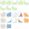 |
Fig. A.1 Histograms of the observables (x) and interior structure parameters (y) that constitute the synthetic dataset used for the training and validation of the neural network. Note that the absolute frequencies of the observables (x) are shown on a logarithmic scale. |
References
- Abadi, M., Barham, P., Chen, J., et al. 2016, in Proceedings of the 12th USENIX Conference on Operating Systems Design and Implementation, OSDI’16 (USA: USENIX Association), 265 [Google Scholar]
- Acuna, M. H., & Ness, N. F.1976, J. Geophys. Res., 81, 2917 [Google Scholar]
- Agarwal, S., Tosi, N., Kessel, P., et al. 2021, Earth Space Sci., 8, e01484 [Google Scholar]
- Anderson, J. D., Lau, E. L., Sjogren, W. L., Schubert, G., & Moore, W. B.1996, Nature, 384, 541 [Google Scholar]
- Andrade, E. N. D. C.1910, Proc. Roy. Soc. Lond. Ser. A, 84, 1 [NASA ADS] [CrossRef] [Google Scholar]
- Atkins, S., Valentine, A. P., Tackley, P. J., & Trampert, J.2016, Phys. Earth Planet. Interiors, 257, 171 [CrossRef] [Google Scholar]
- Baland, R.-M., & Van Hoolst, T.2010, Icarus, 209, 651 [Google Scholar]
- Baland, R.-M., Yseboodt, M., & Hoolst, T. V.2012, Icarus, 220, 435 [NASA ADS] [CrossRef] [Google Scholar]
- Baumeister, P., Padovan, S., Tosi, N., et al. 2020, ApJ, 889, 42 [Google Scholar]
- Bills, B. G.2005, Icarus, 175, 233 [Google Scholar]
- Biot, M. A.1954, J. Appl. Phys., 25, 1385 [Google Scholar]
- Bishop, C.1994, Mixture density networks, Working paper, Aston University [Google Scholar]
- Burša, M.1997, Acta Geodaet. Geophys. Hung., 32, 225 [Google Scholar]
- Caldiero, A., Le Maistre, S., & Dehant, V.2023, in LPI Contributions, 2851, Asteroids, Comets, Meteors Conference, 2583 [Google Scholar]
- Cappuccio, P., Hickey, A., Durante, D., et al. 2020, Planet. Space Sci., 187, 104902 [NASA ADS] [CrossRef] [Google Scholar]
- Cassini, J.-D.1693, De l’Origine et du progrès de l’astronomie et de son usage dans la géographie et dans la navigation (Paris) [Google Scholar]
- Chollet, F.2017, Deep Learning with Python (New York: Manning Publications Co.) [Google Scholar]
- Colombo, G.1966, AJ, 71, 891 [Google Scholar]
- Comstock, R. L., & Bills, B. G.2003, J. Geophys. Res. (Planets), 108, 5100 [Google Scholar]
- Consorzi, A., Melini, D., González-Santander, J. L., & Spada, G.2024, Earth Space Sci., 11, e2024EA003779 [Google Scholar]
- Fort, S., Hu, H., & Lakshminarayanan, B.2020, arXiv e-prints [arXiv:1912.02757] [Google Scholar]
- Fung, Y. C.1965, Foundations of Solid Mechanics, International Series on Dynamics (Englewood Cliffs, N.J.: Prentice-Hall), 539 [Google Scholar]
- Gal, Y., & Ghahramani, Z.2016, in Proceedings of Machine Learning Research, 48, Proceedings of The 33rd International Conference on Machine Learning, eds. M. F.Balcan & K. Q.Weinberger (New York, New York, USA: PMLR), 1050 [Google Scholar]
- Gao, P., & Stevenson, D. J.2013, Icarus, 226, 1185 [NASA ADS] [CrossRef] [Google Scholar]
- Gevorgyan, Y., Boué, G., Ragazzo, C., Ruiz, L. S., & Correia, A. C. M.2020, Icarus, 343, 113610 [NASA ADS] [CrossRef] [Google Scholar]
- Gomez Casajus, L., Ermakov, A. I., Zannoni, M., et al. 2022, Geophys. Res. Lett., 49, e2022GL099475 [NASA ADS] [CrossRef] [Google Scholar]
- Goodfellow, I., Bengio, Y., & Courville, A.2016, Deep Learning (MIT Press) [Google Scholar]
- Hussmann, H., Choblet, G., Lainey, V., et al. 2010, Space Sci. Rev., 153, 317 [CrossRef] [Google Scholar]
- Hussmann, H., Shoji, D., Steinbrügge, G., Stark, A., & Sohl, F.2016, Celest. Mech. Dyn. Astron., 126, 131 [NASA ADS] [CrossRef] [Google Scholar]
- Jara-Orué, H., & Vermeersen, B.2016, Neth. J. Geosci., 95, 191 [Google Scholar]
- Kamata, S., Kimura, J., Matsumoto, K., et al. 2016, J. Geophys. Res. (Planets), 121, 1362 [Google Scholar]
- Kingma, D. P., & Ba, J.2014, arXiv e-prints [arXiv:1412.6980] [Google Scholar]
- Kivelson, M. G., Khurana, K. K., Russell, C. T., et al. 1996, Nature, 384, 537 [NASA ADS] [CrossRef] [Google Scholar]
- Kivelson, M. G., Khurana, K. K., & Volwerk, M.2002, Icarus, 157, 507 [CrossRef] [Google Scholar]
- Käufl, P., P., Valentine, A., W.de Wit, R., & Trampert, J.2016, Geophys. J. Int., 205, 1710 [Google Scholar]
- Loshchilov, I., & Hutter, F.2017, arXiv e-prints, [arXiv:1711.05101] [Google Scholar]
- Love, A. E. H.1909, MNRAS, 69, 476 [NASA ADS] [Google Scholar]
- Melini, D., Saliby, C., & Spada, G.2022, Geophys. J. Int., 231, 1502 [NASA ADS] [CrossRef] [Google Scholar]
- Mitri, G., Meriggiola, R., Hayes, A., et al. 2014, Icarus, 236, 169 [CrossRef] [Google Scholar]
- Moore, W. B., & Schubert, G.2000, Icarus, 147, 317 [NASA ADS] [CrossRef] [Google Scholar]
- Moore, W. B., & Schubert, G.2003, Icarus, 166, 223 [Google Scholar]
- Murray, C. D., & Dermott, S. F.1999, Solar System Dynamics (Cambridge University Press) [Google Scholar]
- Parkinson, W. D.1983, Introduction to Geomagnetism (New York, NY: Elsevier Science Pub. Co., Inc.) [Google Scholar]
- Peltier, W. R.1974, Revi. Geophys. Space Phys., 12, 649 [Google Scholar]
- Petricca, F., Genova, A., Castillo-Rogez, J. C., et al. 2023, Geophys. Res. Lett., 50, e2023GL104016 [NASA ADS] [CrossRef] [Google Scholar]
- Petricca, F., Tharimena, S., Melini, D., et al. 2024, Icarus, 417, 116120 [Google Scholar]
- Prechelt, L.1998, Neural Netw., 11, 761 [Google Scholar]
- Rambaux, N., van Hoolst, T., & Karatekin, Ö.2011, A&A, 527, A118 [NASA ADS] [CrossRef] [EDP Sciences] [Google Scholar]
- Sambridge, M., & Mosegaard, K.2002, Rev. Geophys., 40, 3 [Google Scholar]
- Schubert, G., Zhang, K., Kivelson, M. G., & Anderson, J. D.1996, Nature, 384, 544 [Google Scholar]
- Seufert, M., Saur, J., & Neubauer, F. M.2011, Icarus, 214, 477 [Google Scholar]
- Shida, T.1912, Proceedings of the Tokyo Mathematico-Physical Society 2nd Series, 6, 242 [Google Scholar]
- Sohl, F., Spohn, T., Breuer, D., & Nagel, K.2002, Icarus, 157, 104 [Google Scholar]
- Spada, G., & Boschi, L.2006, Geophys. J. Int., 166, 309 [Google Scholar]
- Spohn, T., & Schubert, G.2003, Icarus, 161, 456 [NASA ADS] [CrossRef] [Google Scholar]
- Srivastava, S. P.1966, Geophys. J., 11, 373 [Google Scholar]
- Srivastava, N., Hinton, G., Krizhevsky, A., Sutskever, I., & Salakhutdinov, R.2014, J. Mach. Learn. Res., 15, 1929 [Google Scholar]
- Stark, A., Oberst, J., Preusker, F., et al. 2015, Planet. Space Sci., 117, 64 [Google Scholar]
- Steinbrügge, G., Stark, A., Hussmann, H., Sohl, F., & Oberst, J.2015, Planet. Space Sci., 117, 184 [Google Scholar]
- Steinbrügge, G., Steinke, T., Thor, R., Stark, A., & Hussmann, H.2019, Geosciences, 9, 320 [Google Scholar]
- Thor, R. N., Kallenbach, R., Christensen, U. R., et al. 2021, J. Geodesy, 95, 4 [Google Scholar]
- Van Hoolst, T., Rambaux, N., Karatekin, Ö., Dehant, V., & Rivoldini, A.2008, Icarus, 195, 386 [Google Scholar]
- Van Hoolst, T., Rambaux, N., Karatekin, Ö., & Baland, R. M.2009, Icarus, 200, 256 [Google Scholar]
- Van Hoolst, T., Tobie, G., Vallat, C., et al. 2024, Space Sci. Rev., 220, 54 [Google Scholar]
- Vance, S., Bouffard, M., Choukroun, M., & Sotin, C.2014, Planet. Space Sci., 96, 62 [Google Scholar]
- Vance, S. D., Styczinski, M. J., Bills, B. G., et al. 2021, J. Geophys. Res. (Planets), 126, e06418 [Google Scholar]
- Verdoja, F., & Kyrki, V.2020, arXiv e-prints, [arXiv:2008.02627] [Google Scholar]
- Wahr, J. M., Zuber, M. T., Smith, D. E., & Lunine, J. I.2006, J. Geophys. Res. (Planets), 111, E12005 [Google Scholar]
- Walterová, M., Plesa, A.-C., Wagner, F. W., & Breuer, D.2023, ESS Open Archive eprints, 992, 169008299.99203183 [Google Scholar]
- Zimmer, C., Khurana, K. K., & Kivelson, M. G.2000, Icarus, 147, 329 [NASA ADS] [CrossRef] [Google Scholar]
- Zubarev, A., Nadezhdina, I., Oberst, J., Hussmann, H., & Stark, A.2015, Planet. Space Sci., 117, 246 [Google Scholar]
All Tables
Values of the representative set of parameters (x*) drawn from the validation dataset.
All Figures
|
Fig. 1 Schematic illustration of an interior structure model of Ganymede, consisting of five concentric layers: an icy shell, a subsurface ocean, HP ice, a silicate mantle, and a fluid core. |
| In the text | |
|
Fig. 2 Schematic representation of the neural network used in this work. On the left we have the input layer with the observable parameters (x), in the middle the four hidden layers, and on the right the output layer constituted by the internal structure parameters (y). A black cross indicates nodes that have been disabled by the dropout layers. |
| In the text | |
|
Fig. 3 Comparison of the actual values of the interior structure parameters (y) with those predicted by the neural network for the validation dataset |
| In the text | |
|
Fig. 4 Comparison of the actual observables (x) in the validation dataset with the corresponding observables ( |
| In the text | |
|
Fig. 5 Histograms of the distribution of the interior structure parameters |
| In the text | |
|
Fig. A.1 Histograms of the observables (x) and interior structure parameters (y) that constitute the synthetic dataset used for the training and validation of the neural network. Note that the absolute frequencies of the observables (x) are shown on a logarithmic scale. |
| In the text | |
Current usage metrics show cumulative count of Article Views (full-text article views including HTML views, PDF and ePub downloads, according to the available data) and Abstracts Views on Vision4Press platform.
Data correspond to usage on the plateform after 2015. The current usage metrics is available 48-96 hours after online publication and is updated daily on week days.
Initial download of the metrics may take a while.