| Issue |
A&A
Volume 699, July 2025
|
|
|---|---|---|
| Article Number | A29 | |
| Number of page(s) | 11 | |
| Section | Atomic, molecular, and nuclear data | |
| DOI | https://doi.org/10.1051/0004-6361/202554230 | |
| Published online | 27 June 2025 | |
Structure, electronic collision, quantum, and semiclassical Stark broadening data for Nb V lines
1
LUX, Observatoire de Paris, Université PSL, Sorbonne Université, CNRS,
92190
Meudon,
France
2
Physics Department, College of Sciences, Umm Al-Qura University,
21955
Makkah Almukarramah,
Saudi Arabia
★ Corresponding authors: This email address is being protected from spambots. You need JavaScript enabled to view it.
; This email address is being protected from spambots. You need JavaScript enabled to view it.
Received:
22
February
2025
Accepted:
22
May
2025
Abstract
Context. We provide structure, electron collision, and Stark broadening parameters of the Rb-like niobium ion Nb V. These data are mandatory for the spectral analysis of hot star spectra after the discovery of many lines of trans-iron elements in hot white dwarfs. To the best of our knowledge, the present results are the first to be published.
Aims. Recently, and for the first time, several lines of trans-iron elements with ionization stages IV through VII from Zn to Ba (Z = 30–56) have been discovered in the ultraviolet spectra of the atmospheres of a DAO-type white dwarf BD-22∘3467, a DA-type white dwarf G191–B2B and a DO-type white dwarf RE 0503–289. This finding motivates us to evaluate the atomic and Stark broadening data of the Nb V ion (Z = 41), required to investigate its abundance and to interpret and analyze the observed spectra.
Methods. We used our quantum method to calculate the Stark widths. The first step of the method consisted in calculating the structure and collision parameters. In a second step, these parameters entered our codes of line broadening calculations to provide the Stark line widths. Since the accuracy of the line width results is related to the accuracy of the collision parameters, we checked the convergence of our collision results during the calculation.
Results. We provide the widths of 30 Nb V lines at different electron temperatures and at an electron density Ne = 1017 cm−3. We compare our result with those obtained using the approximate formula of Cowley and find that rigorous calculations must be performed to obtain accurate Stark widths. We mention also that the Stark broadening mechanism is preponderant for almost all the physical conditions of the considered plasma.
Key words: atomic data / atomic processes / line: profiles / scattering / stars: AGB and post-AGB / stars: atmospheres
© The Authors 2025
 Open Access article, published by EDP Sciences, under the terms of the Creative Commons Attribution License (https://creativecommons.org/licenses/by/4.0), which permits unrestricted use, distribution, and reproduction in any medium, provided the original work is properly cited.
This article is published in open access under the Subscribe to Open model. This email address is being protected from spambots. You need JavaScript enabled to view it. to support open access publication.
1 Introduction
Atomic data, such as energy levels, oscillator strengths, radiative decay rates, and broadening of spectral lines of elements, are crucial tools in astrophysical and laboratory plasma studies, offering valuable insights for various research purposes. For laboratory plasmas, line broadening can be a powerful tool in the modeling of laser-produced and inertial fusion plasma. In astrophysics, they are used in the investigations of radiative transfer, determination of chemical abundances, and stellar opacity calculations. Data for heavy elements, unlike those for light elements, are particularly significant due to their limited availability and the difficulty of their calculations. Many papers (Rauch et al. 2017; Werner et al. 2018; Löbling et al. 2020) and recently (Landstorfer et al. 2024) point out the existence of heavy elements (trans-iron elements: Zn, Ga, Ge, Se, Br, Kr, Sr, Zr, Mo, In, Te, I, Xe, and Ba; and iron-group elements: from calcium to nickel) in white dwarfs and their importance in plasma diagnostics. The atomic data and Stark broadening data of these heavy ions must be taken into account for the spectral analysis; otherwise, restricting ourselves to the atomic data of hydrogen and helium will compromise the results and limit the precision of synthetic spectra.
The continuous development of powerful and high-capacity computers enables precise and advanced calculations of more complex atomic systems, making the theoretical evaluation of atomic and line broadening data for heavy elements (highly ionized elements with high nuclear charges Z) possible. In parallel with computer developments, instruments of astrophysical observations such as the Goddard High Resolution Spectrograph (GHRS) on the Hubble Space Telescope and the Far Ultraviolet Spectroscopic Explorer (FUSE) have enabled the collection of a broad range of spectroscopic data at different physical conditions that can be compared with the theoretical ones.
The broadening of spectral lines is due to many effects: Natural broadening is a consequence of the Heisenberg uncertainty principle. Doppler broadening is due to the distribution of velocities of atoms or molecules. The broadening resulting from the charged particles in a plasma is called Stark broadening; and that resulting from neutral atoms is called Van der Waals broadening. If the neutral atoms are the same, the phenomenon is called resonance broadening. It has been shown that Stark broadening is the most important in many astrophysical objects (Aloui et al. 2022; Elabidi 2021a; Sahal-Bréchot & Elabidi 2021; Dimitrijević 2020; Aloui et al. 2019) because it occurs under widely different plasma physical conditions.
Lines of elements with high ionization stages (IV-VII) have been detected in the spectra of white dwarf (G191–B2B, RE 0503–289, and BD-22°3467) and subdwarf (HZ 44 and HD 127493) stars (Rauch et al. 2016; Rauch et al. 2017; Dorsch et al. 2019). In this work, we focus on the element niobium, and specifically on the Stark broadening and atomic data of the Nb V ion. It is obvious that precise and reliable atomic data are the principal input for any atmosphere modeling. Oscillator strengths and transition probabilities are required for the complete model atoms, not only for the lines identified in an observation (Rauch et al. 2020; Landstorfer et al. 2024). The estimation of the electron collisional rate coefficients and photoionization cross sections requires a complete knowledge of oscillator strengths (Orban et al. 2006). Line strengths and oscillator strengths are required for Stark broadening evaluation (Alonso-Medina & Colón 2014). Even though there are many atomic databases, such as NIST (Kramida et al. 2024), CHIANTI (Del Zanna et al. 2021), the Opacity Project (Seaton et al. 1994), and Kurucz (Kurucz 2018), atomic data are missing, especially for higher ionization stages. Regarding the Stark broadening parameters, the problem is worse for these ions, since their calculations depend on the availability of these preliminary atomic data (energy levels, oscillator strengths, and line strengths). Atomic data for the Nb V ion are scarce, and Stark broadening data are totally missing from the literature, even though research on this ion began very early: we can cite the work of Lindgård & Nielson (1977), in which transition probabilities, oscillator strengths, and lifetimes of Nb V were calculated using a numerical Coulomb approximation. Migdalek & Baylis (1979) calculated oscillator strengths for the lowest ![Mathematical equation: $\[5 \mathrm{S}_{1 / 2}{-}5 \mathrm{P}_{1 / 2,3 / 2}^{\circ}\]$](/articles/aa/full_html/2025/07/aa54230-25/aa54230-25-eq1.png) transitions for Rb-like ions, including Nb V. Zilitis (2007, 2009) calculated new oscillator strengths for the Nb V transitions 5S–5P, 5P–4,5 D, 4D–nP, and 4D3/2–nF5/2 using the Dirac-Fock method. Das et al. (2018) calculated lifetimes and oscillator strengths for Y III to Tc VII transitions. The more recent spectroscopy data can be found in Jyoti et al. (2021), in which line strengths, transition probabilities, and oscillator strengths for the allowed transitions involving the levels
transitions for Rb-like ions, including Nb V. Zilitis (2007, 2009) calculated new oscillator strengths for the Nb V transitions 5S–5P, 5P–4,5 D, 4D–nP, and 4D3/2–nF5/2 using the Dirac-Fock method. Das et al. (2018) calculated lifetimes and oscillator strengths for Y III to Tc VII transitions. The more recent spectroscopy data can be found in Jyoti et al. (2021), in which line strengths, transition probabilities, and oscillator strengths for the allowed transitions involving the levels ![Mathematical equation: $\[n \mathrm{S}_{1 / 2}, n \mathrm{P}_{1 / 2,3 / 2}^{\circ}\]$](/articles/aa/full_html/2025/07/aa54230-25/aa54230-25-eq2.png) , and n′D3/2,5/2, with n = 5 to 10 and n′ = 4 to 10 of the Rb-like ions Zr IV and Nb V were calculated.
, and n′D3/2,5/2, with n = 5 to 10 and n′ = 4 to 10 of the Rb-like ions Zr IV and Nb V were calculated.
We concentrate on Stark broadening in this work and calculate the Nb V line widths using our quantum formalism (Elabidi et al. 2004, 2008) and semiclassical perturbation (SCP) formalism. The SCP theory, which involves hyperbolic trajectories for ionized radiating atoms, has been developed and updated by Sahal-Brechot (1969a,b); Sahal-Bréchot (1974); Fleurier et al. (1977); Sahal-Bréchot (2021). The resulting SCP code has been continually improved and used since 1984 (for example, Dimitrijević et al. (2011)). The theory was revisited by Sahal-Bréchot et al. (2014); Sahal-Bréchot & Elabidi (2021). The two results are compared and presented at various temperatures, which are useful for many astrophysical purposes. The SCP method was shown to be sufficiently precise for the needs and agrees with other theoretical methods and experimental results. The uncertainty in the SCP results is due to the use of the perturbation theory in the evaluation of the close collision contribution to the line widths. Our quantum method has been applied in recent years to several ions (Aloui et al. 2024a,b,c; Elabidi et al. 2023a,b; Aloui et al. 2022; Elabidi 2021a,b; Sahal-Bréchot & Elabidi 2021), and whenever experimental or other theoretical results are available, we have achieved good agreement in almost all cases. This motivates us to extend our calculations to determine missing line broadening data for the Nb V ion, which will be useful for astrophysicists. Since Stark broadening parameters for the considered ion are totally missing from the literature, the only way to check their accuracy is to verify the reliability of the data used to calculate the line widths, such as energy levels, oscillator strengths, and wavelengths, and to test the convergence of the collision parameters, such as collision strengths or cross sections, with the electron energy. So, besides the final Stark broadening data, we show a comparison between our preliminary data and those of Jyoti et al. (2021), and we present an extensive study of the convergence of our results. We also use the approximated formula of Cowley (1971) to produce the Stark broadening of the 30 lines and compare them with our rigorous calculations. The agreement between the two results is not conclusive, indicating that when exact calculations can be performed, it is not recommended to use the approximated formula of Cowley (1971).
Our paper is structured as follows: Section 2 is dedicated to a brief description of the method used for the evaluation of Stark broadening data. Results of the atomic data and their comparisons are presented in Sect. 3 together with a discussion about the convergence of our collision strengths. Results for the line widths are presented in Sect. 4, along with comparisons to the Cowley formula. Finally, we summarize our results and conclude in Sect. 5.
2 Description of the theory and computational procedure
Our quantum method for electron impact broadening is well described in Elabidi et al. (2004, 2008); Aloui et al. (2018). Here, we present only an overview. In Elabidi et al. (2004, 2008), we considered fine structure effects and relativistic corrections resulting from the nonvalidity of the LS coupling approximation for the target by using the intermediate coupling scheme. We derived the formula of the full width at half maximum (FWHM), W, expressed in angular frequency units of a spectral line arising from a transition from an upper level, i, to a lower level, f, (Elabidi et al. 2008) with
![Mathematical equation: $\[W=2 N_e\left(\frac{\hbar}{m}\right)^2\left(\frac{m \pi}{2 k_B T}\right)^{\frac{1}{2}} \int_0^{\infty} \Gamma_{i \rightarrow f}^w(\epsilon) \exp \left(\frac{-\epsilon}{k_B T}\right) \mathrm{d}\left(\frac{\epsilon}{k_B T}\right),\]$](/articles/aa/full_html/2025/07/aa54230-25/aa54230-25-eq3.png) (1)
(1)
where the integral is performed using a trapezoid method with an increasing energy step. Here, m is the electron mass, kB the Boltzmann constant, Ne the electron density, T the electron temperature, ϵ the incident electron energy, and
![Mathematical equation: $\[\begin{aligned}\Gamma_{i \rightarrow f}^w(\epsilon)= & \sum_{\substack{J_i^T J_f^T \\\ell K_i K_f}} \frac{\left(2 K_i+1\right)\left(2 J_i^T+1\right)\left(2 K_f+1\right)\left(2 J_f^T+1\right)}{2} \\& \times\left\{\begin{array}{c}J_i K_i \ell \\K_f J_f 1\end{array}\right\}^2\left\{\begin{array}{c}K_i J_i^T s \\J_f^T K_f 1\end{array}\right\}^2 \\& \times\left[1-\left(\Re\left(\mathbb{S}_i\right) \Re\left(\mathbb{S}_f\right)+\mathfrak{J}\left(\mathbb{S}_i\right) \mathfrak{J}\left(\mathbb{S}_f\right)\right)\right],\end{aligned}\]$](/articles/aa/full_html/2025/07/aa54230-25/aa54230-25-eq4.png) (2)
(2)
where Lj+Sj =Jj, Jj+ℓ =Kj and ![Mathematical equation: $\[K_{j}+s=J_{j}^{T}\]$](/articles/aa/full_html/2025/07/aa54230-25/aa54230-25-eq5.png) (j = i or f). L and S are the orbital and spin momenta of the emitter; ℓ and s are those of the perturber (electron); and all the parameters denoted by T refer to the system of electron+ion. 𝕊j, ℜ(𝕊j), and ℑ(𝕊j) are the scattering matrix elements and their real and imaginary parts for the level j (j = i or f). These matrices are written in the basis of the intermediate coupling scheme and evaluated at the same perturber energy,
(j = i or f). L and S are the orbital and spin momenta of the emitter; ℓ and s are those of the perturber (electron); and all the parameters denoted by T refer to the system of electron+ion. 𝕊j, ℜ(𝕊j), and ℑ(𝕊j) are the scattering matrix elements and their real and imaginary parts for the level j (j = i or f). These matrices are written in the basis of the intermediate coupling scheme and evaluated at the same perturber energy, ![Mathematical equation: $\[\epsilon=\frac{1}{2} m v^{2}\]$](/articles/aa/full_html/2025/07/aa54230-25/aa54230-25-eq6.png) . In addition,
. In addition, ![Mathematical equation: $\[\left\{\begin{array}{c}a b c \\ d e f\end{array}\right\}\]$](/articles/aa/full_html/2025/07/aa54230-25/aa54230-25-eq7.png) are the 6–j symbols.
are the 6–j symbols.
To evaluate the expression (2) of ![Mathematical equation: $\[\Gamma_{i \rightarrow f}^{w}\]$](/articles/aa/full_html/2025/07/aa54230-25/aa54230-25-eq8.png) , we need to calculate ℜ(𝕊) and ℑ(𝕊) for the initial i and final f levels. This task is performed using the UCL codes: SUPERSTRUCTURE (SST) of Eissner et al. (1974) for the structure calculations (energy levels, oscillator strengths, etc.), in addition to the term coupling coefficients (TCCs), which will be used in the scattering part (Elabidi et al. 2004) through the codes DISTORTED WAVE (DW) of Eissner (1998) and JAJOM (Saraph 1978). In the present work, we transformed JAJOM into JAJPOLARI (Elabidi & Dubau, unpublished results) and RTOS (Dubau, unpublished results) to produce the real ℜ(𝕊) and the imaginary ℑ(𝕊) parts of the scattering matrix entering our code to evaluate the expression (2). We included in our calculations Feshbach resonances using the Gailitis method (Gailitis 1963). The factor,
, we need to calculate ℜ(𝕊) and ℑ(𝕊) for the initial i and final f levels. This task is performed using the UCL codes: SUPERSTRUCTURE (SST) of Eissner et al. (1974) for the structure calculations (energy levels, oscillator strengths, etc.), in addition to the term coupling coefficients (TCCs), which will be used in the scattering part (Elabidi et al. 2004) through the codes DISTORTED WAVE (DW) of Eissner (1998) and JAJOM (Saraph 1978). In the present work, we transformed JAJOM into JAJPOLARI (Elabidi & Dubau, unpublished results) and RTOS (Dubau, unpublished results) to produce the real ℜ(𝕊) and the imaginary ℑ(𝕊) parts of the scattering matrix entering our code to evaluate the expression (2). We included in our calculations Feshbach resonances using the Gailitis method (Gailitis 1963). The factor, ![Mathematical equation: $\[\Gamma_{i \rightarrow f}^{w}\]$](/articles/aa/full_html/2025/07/aa54230-25/aa54230-25-eq9.png) , was extrapolated below the threshold energy for the corresponding inelastic process. It was shown in Elabidi et al. (2009) that including Feshbach resonances in the calculation of line widths leads to better agreement with experimental results, especially at low temperatures.
, was extrapolated below the threshold energy for the corresponding inelastic process. It was shown in Elabidi et al. (2009) that including Feshbach resonances in the calculation of line widths leads to better agreement with experimental results, especially at low temperatures.
Energies (E1) in cm−1 of the 14 lowest Nb V levels compared with RMBPT(a) (E2) and NIST(b) results.
3 Atomic structure and electron–ion scattering
3.1 Atomic structure
For the study of the structure and collision of the Nb V ion, we used eight electronic configurations: [Kr] 4d, 5s, 5p, 5d, 4f, 6s, 6p, and 6d. The structure calculations were performed using the SST code of Eissner et al. (1974), where the wave functions are determined by the diagonalization of the nonrelativistic Hamiltonian using orbitals calculated in scaled Thomas–Fermi–Dirac–Amaldi (TFDA) potentials. Relativistic corrections (spin–orbit, mass, Darwin, and one-body) were introduced according to the Breit–Pauli approach (Bethe & Salpeter 1957) in LSJ coupling. The wave functions were used to determine the energies and other radiative atomic data. The absorption oscillator strengths, fl→u, and the radiative decay rates, Aul, of the allowed transitions (E1) between the upper (u) and lower (l) levels are given by
![Mathematical equation: $\[f_{l \rightarrow u}=\frac{303.756}{g_l \lambda} S^{[E 1]} \quad \text { and } \quad A_{u l}=\frac{2.0261269 \times 10^{18}}{g_u \lambda^3} S^{[E 1]},\]$](/articles/aa/full_html/2025/07/aa54230-25/aa54230-25-eq17.png) (3)
(3)
where S[E1] is the line strength defined as the square of the transition moment ⟨ψl|μ|ψu⟩, μ is the electric dipole moment operator for permitted transitions, g refers to the statistical weights, and λ is the wavelength in Å.
The SST code takes into account configuration interactions and relativistic corrections (spin–orbit, mass, Darwin, and onebody) introduced according to the Breit–Pauli approach (Bethe & Salpeter 1957) in LSJ coupling. However, it does not account for core-polarization and core-penetration effects. Quinet et al. (1999) mentioned that for complex ions, these effects must be introduced to obtain more accurate oscillator strengths. Meléndez et al. (2007) showed that polarization interaction affects the oscillator strengths by up to 12% and affects the lifetimes and effective collision strengths by about 20%. Concerning Stark broadening, which is the aim of this work, Hamdi et al. (2013) calculated SCP Stark widths for the Pb IV ion using three sets of wighted oscillator strengths (g * f). They performed an extensive comparison of the results obtained with different oscillator strengths. The three methods used to calculate g * f are the following: the HFR correction approach using the Cowan code (Cowan 1981), the third-order many-body perturbation theory (Safronova & Johnson 2004) with core-polarization effects from Chou & Johnson (1997), and the relativistic Hartree-Fock calculations in intermediate coupling (Alonso-Medina et al. 2011) including the core-polarization effects from Migdalek & Baylis (1979). They also compared their results to previous SCP ones (Dimitrijević & Sahal-Bréchot 1999) obtained using the oscillator strengths of Bates & Damgaard (1949). They found that the effect of oscillator strengths is about 20%. This value is not crucial, since it is roughly of the same order of magnitude as the accuracy of the SCP method. Furthermore, in our quantum method, Stark widths are less sensitive to oscillator strengths than in the SCP method. So, we can conclude that neglecting core polarization in the evaluation of oscillator strengths slightly reduces their accuracy but does not significantly affect the accuracy of our quantum Stark widths.
We present in Table 1 the fine structure levels obtained from the eight configurations together with the results measured by Kagan et al. (1981) and taken from the National Institute of Standards and Technology (NIST) database (Kramida et al. 2024), as well as those from Jyoti et al. (2021), obtained using the relativistic many-body perturbation theory (RMBPT). The average relative error between the NIST results and the present ones is about 1.27%, while that with the RMBPT results is about 4.18%. This indicates a difference of about 3% between our energies and those of the RMBPT. The radiative data (wavelengths λ, absorption oscillator strengths fl→u, radiative decay rates Aul, and line strengths S) for the possible electric dipole transitions involving the 14 levels are presented in Table 2. The obtained results are compared only with the RMBPT data (Jyoti et al. 2021), since no NIST radiative data are available. The wavelengths of the two calculations are in good agreement for all the transitions with an average error of about 1.4%. For the oscillator strengths, radiative decay rates, and line strengths, the average relative error is around 22%. Important discrepancies (40–70%) have been reported for six transitions with high energy differences ΔEij (λ ≈ 40–70 nm). These values are marked by an asterisk in Table 2. If we exclude these from the comparison, we obtain an acceptable average error (of about 11%).
Wavelengths (λ1), oscillator strengths (f1), radiative decay rates (A1), and line strengths (S1) compared with RMBPT results (a).
3.2 Electron–ion scattering
In our method, collision is a primary part in the evaluation of the line widths, since Stark broadening is principally caused by collisions between the emitter (ion) and the surrounding electrons. This is why we present here a detailed description of how the collision is treated. This collision calculation was performed using the DW code (Eissner 1998) and the JAJOM code (Saraph 1978). In DW, the collision is treated in LS coupling, with the angular momentum of the colliding electron set up to ℓ = 19. The JAJOM code transforms the reactance matrices, ℝLSπ, from LS coupling (obtained in DW) into JK coupling according to the expression,
![Mathematical equation: $\[\begin{aligned}\mathbb{R}^{J \pi}\left(\gamma_{J K}, \gamma_{J K}^{\prime}, \epsilon_i\right)= & \sum_{L S} C\left(S L J, S_i L_i J_i, \ell K\right) \mathbb{R}^{L S \pi}\left(\gamma_{L S}, \gamma_{L S}^{\prime}, \epsilon_i\right) \\& \times C\left(S L J, S_i^{\prime} L_i^{\prime} J_i^{\prime}, \ell^{\prime} K^{\prime}\right).\end{aligned}\]$](/articles/aa/full_html/2025/07/aa54230-25/aa54230-25-eq18.png) (4)
(4)
We combined all the quantum numbers (same definition as in expression 2, with π referring to the parity) that define the state in JK coupling and those in LS coupling in the form, ![Mathematical equation: $\[\left(\gamma_{J K}, \gamma_{J K}^{\prime}, \epsilon_{i}\right)=\left(\Gamma_{i} S_{i} L_{i} J_{i} \ell K, \Gamma_{i}^{\prime} S_{i}^{\prime} L_{i}^{\prime} J_{i}^{\prime} \ell^{\prime} K^{\prime}; \epsilon_{i}\right)\]$](/articles/aa/full_html/2025/07/aa54230-25/aa54230-25-eq19.png) , and
, and ![Mathematical equation: $\[\left(\gamma_{L S}, \gamma_{L S}^{\prime}, \epsilon_{i}\right)=\left(\Gamma_{i} S_{i} L_{i} \ell s, \Gamma_{i}^{\prime} S_{i}^{\prime} L_{i}^{\prime} \ell^{\prime} s; \epsilon_{i}\right)\]$](/articles/aa/full_html/2025/07/aa54230-25/aa54230-25-eq20.png) , where ΓjSjLj refers to the configuration j. The recoupling terms, C, are related to the Racah coefficients, W, by (Racah 1943):
, where ΓjSjLj refers to the configuration j. The recoupling terms, C, are related to the Racah coefficients, W, by (Racah 1943):
![Mathematical equation: $\[\begin{aligned}C\left(S L J, S_i L_i J_i, \ell K\right)= & W\left(L \ell S_i ; L_i K\right) W\left(L J S_i s ; S K\right) \\& \times\left[(2 S+1)(2 L+1)(2 K+1)\left(2 J_i+1\right)\right]^{1 / 2}.\end{aligned}\]$](/articles/aa/full_html/2025/07/aa54230-25/aa54230-25-eq21.png) (5)
(5)
Finally, we calculated the reactance matrices in intermediate coupling ![Mathematical equation: $\[\mathbb{R}^{J \pi}\left(\gamma_{J K}, \gamma_{J K}^{\prime}, \epsilon_i\right)\]$](/articles/aa/full_html/2025/07/aa54230-25/aa54230-25-eq22.png) by using the TCCs, fJ, obtained from the SST code, through the relation,
by using the TCCs, fJ, obtained from the SST code, through the relation,
![Mathematical equation: $\[\mathbb{R}^{J \pi}\left(\Delta_i J_i \ell K, \Delta_i^{\prime} J_i^{\prime} \ell^{\prime} K^{\prime}\right)=\sum_{S_i L_i S_i^{\prime} L_i^{\prime}} f_{J_i} \mathbb{R}^{J \pi}\left(\gamma_{J K}, \gamma_{J K}^{\prime}\right) f_{J_i^{\prime}},\]$](/articles/aa/full_html/2025/07/aa54230-25/aa54230-25-eq23.png) (6)
(6)
where Δj replaces the set ΓjSjLj indexing the configuration j. These reactance matrices were used to produce the scattering matrices 𝕊 entering the expression of the line widths (2):
![Mathematical equation: $\[\mathbb{S}=\frac{1+i \mathbb{R}}{1-i \mathbb{R}} \Longrightarrow\left\{\begin{array}{l}\Re(\mathbb{S})=\left(1-\mathbb{R}^2\right)\left(1+\mathbb{R}^2\right)^{-1} \\\mathfrak{J}(\mathbb{S})=2 \mathbb{R}\left(1+\mathbb{R}^2\right)^{-1}\end{array}\right..\]$](/articles/aa/full_html/2025/07/aa54230-25/aa54230-25-eq24.png) (7)
(7)
Equations (7) guarantee the unitarity of the scattering matrices, 𝕊.
In general, we present collision parameters as cross sections, ![Mathematical equation: $\[\sigma\left(i, i^{\prime}\right)=\frac{\pi a_{0}^{2}}{g_{i} \epsilon_{i}} \Omega\left(i, i^{\prime}\right)\]$](/articles/aa/full_html/2025/07/aa54230-25/aa54230-25-eq25.png) , where ϵi is the energy of the incident electron relative to the level i, expressed in Rydbergs, and Ω(i, i′) is the collision strength. Unlike cross sections, collision strengths are symmetric with respect to the levels i and i′. They are given by the following expression using the transition matrices 𝕋 = 1 − 𝕊:
, where ϵi is the energy of the incident electron relative to the level i, expressed in Rydbergs, and Ω(i, i′) is the collision strength. Unlike cross sections, collision strengths are symmetric with respect to the levels i and i′. They are given by the following expression using the transition matrices 𝕋 = 1 − 𝕊:
![Mathematical equation: $\[\begin{aligned}\Omega\left(\Gamma_i L_i S_i J_i ; \Gamma_i^{\prime} L_i^{\prime} S_i^{\prime} J_i^{\prime}\right)= & \frac{1}{2} \sum_{J \pi}(2 J+1) \\& \times \sum_{\ell \ell^{\prime}}\left|\mathbb{T}^{J \pi}\left(\Gamma_i L_i S_i J_i \ell K ; \Gamma_i^{\prime} L_i^{\prime} S_i^{\prime} J_i \ell^{\prime} K^{\prime}\right)\right|^2.\end{aligned}\]$](/articles/aa/full_html/2025/07/aa54230-25/aa54230-25-eq26.png) (8)
(8)
The collision strength, ΩLS, is a sum of the partial collision strengths, ΩJ, according to the expression,
![Mathematical equation: $\[\Omega\left(\Gamma_i L_i S_i ; \Gamma_i^{\prime} L_i^{\prime} S_i^{\prime}\right)=\sum_{J_i J_i^{\prime}} \Omega\left(\Gamma_i L_i S_i J_i ; \Gamma_i^{\prime} L_i^{\prime} S_i^{\prime} J_i^{\prime}\right).\]$](/articles/aa/full_html/2025/07/aa54230-25/aa54230-25-eq27.png) (9)
(9)
This relation is used as a tool to check the convergence of the collision results as well as the accuracy of our calculated line widths.
We present in Table 3 the collision strengths, Ω(i, i′), for the transitions involving the levels i = 1, 2, 3 and i′ = 2–14 at incident electron energies E = 5, 10, 20, 30, 40 and 60 Ryd. To the best of our knowledge, there are no other results of collision strengths to compare with. However, as seen in Fig. 1, the collision strengths converge for all the illustrative transitions. In Fig. 1 (panel a), we display the optically forbidden transitions: 4d 2D3/2−4d 2D5/2 (1–2), 4d 2D3/2−5s 2S1/2 (1–3), and ![Mathematical equation: $\[5 \mathrm{s}~^{2} \mathrm{S}_{1 / 2}-4 \mathrm{f} ~^{2} \mathrm{F}_{5 / 2}^{o}\]$](/articles/aa/full_html/2025/07/aa54230-25/aa54230-25-eq28.png) (3–8). As expected, their collision strengths easily converge at low energies. In Fig. 1 (panel b), we display the collision strengths of the optically allowed transitions
(3–8). As expected, their collision strengths easily converge at low energies. In Fig. 1 (panel b), we display the collision strengths of the optically allowed transitions ![Mathematical equation: $\[4 \mathrm{d}~^{2} \mathrm{D}_{3 / 2}{-}4 \mathrm{f}~^{2} \mathrm{F}_{5 / 2}^{\mathrm{o}}\]$](/articles/aa/full_html/2025/07/aa54230-25/aa54230-25-eq29.png) (1–8),
(1–8), ![Mathematical equation: $\[4\mathrm{d} ^~{2} \mathrm{D}_{5 / 2}{-}4 \mathrm{f}~^{2} \mathrm{F}_{7 / 2}^{\mathrm{o}}\]$](/articles/aa/full_html/2025/07/aa54230-25/aa54230-25-eq30.png) (2–9), and
(2–9), and ![Mathematical equation: $\[5 \mathrm{s}~^{2} \mathrm{S}_{1 / 2}{-}5 \mathrm{p}~^{2} \mathrm{P}_{1 / 2}^{\mathrm{o}}\]$](/articles/aa/full_html/2025/07/aa54230-25/aa54230-25-eq31.png) (3–4), which converge at higher energies (about 30 Ryd). As mentioned above, expression (9) can serve as a verification tool for collision strength convergence. This is achieved here by studying the behavior of the partial collision strengths, Ω(J, J′), as a function of the total angular momentum, JT. The results are displayed in Fig. 2 at different incident electron energies for the forbidden transition, 4d 2D3/2−4d 2D5/2 (panel a), and the allowed transition, 4d 2D3/2−4f 2F5/2 (panel b). We can see that for the forbidden transition, the convergence of the collision strength occurs for JT = 13 at energy E = 5 Ryd, and for JT = 23 at energy E = 40 Ryd. Convergence for the allowed transition requires the inclusion of higher total angular momentum. At an energy of 5 Ryd, collision strengths converge for JT = 16, while at E = 40 Ryd, a trend toward convergence begins at JT = 21. The above examination reveals that our collision strengths, as well as the scattering matrices 𝕊, converge for the considered energies and angular momenta. This conclusion helps us have an idea about the convergence and accuracy of our line broadening results, since we use the scattering matrices (related to the collision strengths) in the calculation of line widths.
(3–4), which converge at higher energies (about 30 Ryd). As mentioned above, expression (9) can serve as a verification tool for collision strength convergence. This is achieved here by studying the behavior of the partial collision strengths, Ω(J, J′), as a function of the total angular momentum, JT. The results are displayed in Fig. 2 at different incident electron energies for the forbidden transition, 4d 2D3/2−4d 2D5/2 (panel a), and the allowed transition, 4d 2D3/2−4f 2F5/2 (panel b). We can see that for the forbidden transition, the convergence of the collision strength occurs for JT = 13 at energy E = 5 Ryd, and for JT = 23 at energy E = 40 Ryd. Convergence for the allowed transition requires the inclusion of higher total angular momentum. At an energy of 5 Ryd, collision strengths converge for JT = 16, while at E = 40 Ryd, a trend toward convergence begins at JT = 21. The above examination reveals that our collision strengths, as well as the scattering matrices 𝕊, converge for the considered energies and angular momenta. This conclusion helps us have an idea about the convergence and accuracy of our line broadening results, since we use the scattering matrices (related to the collision strengths) in the calculation of line widths.
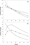 |
Fig. 1 Collision strength as a function of the incident electron energy, E. Panel a: three forbidden transitions 1–2 (∘), 1–3 (•), and 3–8 (*); Panel b: three allowed transitions 1–8 (•), 2–9 (∘), and 3–4 (*). |
4 Stark broadening results
4.1 Quantum and semiclassical perturbation results
In this section, we present our calculated quantum (Q) and SCP Stark widths for 30 spectral lines. The results, displayed in Table A.1, are calculated at an electronic density, Ne = 1017 cm−3, and at five temperatures between 105−106 K. This range of temperature is suitable for astrophysical applications. Spectral lines between fine structure levels are grouped in the table according to their corresponding multiplets. We also present in Table A.1 the relative error between the Q and SCP results. When averaged over all the lines and all the considered temperatures, we find a mean value of about 26%, with a maximum of 60%. We note that, for almost all the lines, the least agreement between the two calculations is found at low temperatures. Furthermore, at these low temperatures, the Q widths are higher than the SCP ones. This is because at low temperatures, elastic collisions and, therefore, close collisions are more important, and the perturbation theory is no longer valid. That is why for this region of energy (temperature), more sophisticated calculations—such as the quantum ones—must be performed to obtain more accurate results. An exception to this conclusion is found for the d–f transitions, where, for all the temperatures, the SCP results are higher than the quantum ones. Furthermore, we find the least agreement between the two results at high temperature. As an illustration of the behavior of the line widths with temperature, we display in Fig. 3 our calculated Q and SCP widths for the two lines: ![Mathematical equation: $\[4 \mathrm{d}~^{2} \mathrm{D}_{3 / 2}{-}4 \mathrm{f}~^{2} \mathrm{F}_{5 / 2}^{\mathrm{o}}\]$](/articles/aa/full_html/2025/07/aa54230-25/aa54230-25-eq32.png) (1–8) in panel a, and
(1–8) in panel a, and ![Mathematical equation: $\[5 \mathrm{s}~^{2} \mathrm{S}_{1 / 2}{-}5 \mathrm{p}~^{2} \mathrm{P}_{1 / 2}^{\mathrm{o}}\]$](/articles/aa/full_html/2025/07/aa54230-25/aa54230-25-eq33.png) (3–4) in panel b, at an electron density Ne = 1017 cm−3. We chose the following lines to show the above conclusions: Panel a displays a d-f transition, where the SCP results are higher than the quantum ones at all the considered temperatures, contrary to the usual behavior observed for the s–p line in the panel b.
(3–4) in panel b, at an electron density Ne = 1017 cm−3. We chose the following lines to show the above conclusions: Panel a displays a d-f transition, where the SCP results are higher than the quantum ones at all the considered temperatures, contrary to the usual behavior observed for the s–p line in the panel b.
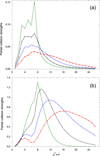 |
Fig. 2 Partial collision strength as a function of the total angular momentum, JT + 1, for the forbidden transition 1–2 (panel a) and for the allowed transition 1–8 (panel b) at four energies: 5 Ryd (Δ), 10 Ryd (×), 20 Ryd (∘), and 40 Ryd (⋆). |
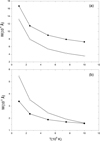 |
Fig. 3 Quantum (∘) and semiclassical perturbation (•) Stark widths of the two transitions |
![Mathematical equation: $\[4 \mathrm{d}~^{2} \mathrm{D}_{3 / 2}{-}4 \mathrm{f}~^{2} \mathrm{F}_{5 / 2}^{\mathrm{o}}\]$](/articles/aa/full_html/2025/07/aa54230-25/aa54230-25-eq34.png)
![Mathematical equation: $\[5 \mathrm{s}~^{2} \mathrm{S}_{1 / 2}{-}5 \mathrm{p}~^{2} \mathrm{P}_{1 / 2}^{\mathrm{o}}\]$](/articles/aa/full_html/2025/07/aa54230-25/aa54230-25-eq35.png)
4.2 Estimation of Stark widths using the Cowley formula
We calculate the Stark widths of the 30 Nb V lines using the Cowley approximate formula (Cowley 1971). The approximate formula is proposed for one electron temperature T = 104 K, and Cowley (1971) mentioned that the formula is not recommended when detailed calculations or experimental results are available. The Stark width WC, expressed in Å, is given by the formula (Cowley 1971)
![Mathematical equation: $\[W_{\mathrm{C}}=1.54 \times 10^{-10} N_e \lambda^2 n_u^{* 4},\]$](/articles/aa/full_html/2025/07/aa54230-25/aa54230-25-eq36.png) (10)
(10)
where Ne is the electron density in cm−3 λ is the wavelength of the considered transition in centimeters, and ![Mathematical equation: $\[n_{u}^{*}\]$](/articles/aa/full_html/2025/07/aa54230-25/aa54230-25-eq37.png) is the effective principal quantum number of the upper level of the transition, defined by
is the effective principal quantum number of the upper level of the transition, defined by
![Mathematical equation: $\[n_u^{* 2}=\frac{E_H Z^2}{E_{ion}-E_u}.\]$](/articles/aa/full_html/2025/07/aa54230-25/aa54230-25-eq38.png) (11)
(11)
Z is the effective charge (Z = 1 for neutral atoms, Z = 2 for singly charged ions,...), EH = 13.606 eV is the ionization energy of the hydrogen, Eu is the energy of the upper level of the transition, and Eion is the ionization energy of the emitter. All energy values are expressed in eV.
Our quantum widths W and those of Cowley WC are presented in Table for two electronic temperatures of 104 K and 2.5 × 10⁴ K, and an electron density of N = 1017 cm−3. Results for T = 2.5 × 10⁴ K are obtained from those at T = 104 K, supposing that widths are proportional to T−1/2 as in our formula 1 and as used in several previous works (Majlinger et al. 2017; Hamdi et al. 2024). Regarding the ratio of our results and those obtained from the Cowley formula (W/WC), we see two groups of lines: a first group where the Cowley approximation overestimates the line widths, with W/WC = 0.28–0.97, and a second group where the approximate formula presents acceptable agreement with our quantum results, with W/WC = 1.01–1.24. This shows that we cannot decide about the accuracy and the applicability of the formula (10), even though we have used this formula at the temperature proposed by Cowley (1971). Consequently, the approximated formula must be used, if necessary, with high caution, especially for temperatures far away from 104 K. We also present in Fig. 4 the spectral shapes of the ![Mathematical equation: $\[5 \mathrm{p}~^{2} \mathrm{P}_{1 / 2}^{\circ}{-}5 \mathrm{d}^{2} \mathrm{D}_{3 / 2}\]$](/articles/aa/full_html/2025/07/aa54230-25/aa54230-25-eq40.png) line (1218.54 Å) using our quantum widths and those obtained from the approximate formula of Cowley (Cowley 1971).
line (1218.54 Å) using our quantum widths and those obtained from the approximate formula of Cowley (Cowley 1971).
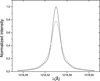 |
Fig. 4 The |
![Mathematical equation: $\[5 \mathrm{p}~^{2} \mathrm{P}_{1 / 2}^{\circ}{-}5 \mathrm{d}^{2} \mathrm{D}_{3 / 2}\]$](/articles/aa/full_html/2025/07/aa54230-25/aa54230-25-eq39.png)
5 Conclusion
In this work, we calculated the Stark broadening of 30 spectral lines of the niobium ion Nb V using both our quantum mechanical method and the semiclassical perturbation method. We presented the results at different electron temperatures and at an electron density of Ne = 1017 cm−3. The comparisons show an overall agreement of about 26%, with higher values reaching 60%. The main reason for this disagreement may be the evaluation of the contributions of the elastic (close) collisions to the line widths by the semiclassical perturbation approach. These contributions occur at low energies (temperatures), which explains why high disagreement is found for almost all the lines at low temperatures. Structure (energy levels and radiative atomic data) and collision strengths used for Stark broadening calculations were also presented. We compared our energies and those of Jyoti et al. (2021) with the results from the NIST database (Kramida et al. 2024). We find that our energies agree with the NIST values within about 1.3%, while those of Jyoti et al. (2021) agree within about 4%. The radiative atomic data (wavelengths, oscillator strengths, radiative decay rates, and line strengths) are compared with the RMBPT results, and a relative error of about 22% is found. A larger difference in radiative atomic data is reported for six transitions with high energy differences, ΔEij (λ ≈ 40–70 nm). If we eliminate these values from the comparison, we find a relative error of about 11%. We also calculate collision strengths at several incident electron energies and are unable to perform comparisons due the lack of available results in the literature. An alternative method to assess the accuracy of these collision data is to check their convergence with respect to the electron energy and the total angular momentum, JT. The results of this test show that collision strengths converge well even at high energies. Since the structure and collision data represent the preliminary input to the Stark broadening calculations, their accuracy is important for obtaining accurate Stark broadening results. We show that Cowley's approximate formula (Cowley 1971) gives results that are not always in good agreement with our rigorous calculations: the ratio, W/WC, varies from 0.28 to 1.24 for the temperatures T = 104 K proposed by (Cowley 1971) and for T = 2.5 × 10⁴ K. A value of 0.28 is found for the d–f transitions. We confirm the statement of Cowley (1971) that his approximate formula is not recommended when more rigorous calculations are performed. Our results, especially the Stark broadening data, will help fill the gap in the STARK-B database (Sahal-Bréchot et al. 2025), which is accessible to astrophysicists. New experimental or theoretical results are welcome to further assess the accuracy of the present calculations.
Acknowledgements
The authors extend their appreciation to Umm Al-Qura University, Saudi Arabia for funding this research work through grant number: 25UQU4331237GSSR01
Funding statement
This research work was funded by Umm Al-Qura University, Saudi Arabia under grant number: 25UQU4331237GSSR01.
Appendix A Additional tables
Our quantum Stark widths (WQ) and our semiclassical perturbation widths (WSCP) of Nb V lines at a density Ne = 1017 cm−3.
Our Nb V line widths (W) and those from the Cowley (1971) approximation at a density Ne = 1017 cm−3. T is expressed in 104 K.
References
- Alonso-Medina, A., & Colón, C. 2014, MNRAS, 445, 1567 [Google Scholar]
- Alonso-Medina, A., Colón, C., & Porcher, P. 2011, At. Data Nucl. Data Tables, 97, 36 [Google Scholar]
- Aloui, R., Elabidi, H., Sahal-Bréchot, S., & Dimitrijević, M. S. 2018, Atoms, 6, 20 [Google Scholar]
- Aloui, R., Elabidi, H., Hamdi, R., & Sahal-Bréchot, S. 2019, MNRAS, 484, 4801 [Google Scholar]
- Aloui, R., Elabidi, H., & Sahal-Bréchot, S. 2022, MNRAS, 512, 1598 [Google Scholar]
- Aloui, R., Elabidi, H., Dimitrijević, M. S., & Sahal-Bréchot, S. 2024a, J. Quant. Spec. Radiat. Transf., 322, 109027 [Google Scholar]
- Aloui, R., Elabidi, H., & Sahal-Bréchot, S. 2024b, J. Quant. Spec. Radiat. Transf., 325, 109084 [Google Scholar]
- Aloui, R., Elabidi, H., Sahal-Bréchot, S., et al. 2024c, J. Quant. Spec. Radiat. Transf., 314, 108867 [Google Scholar]
- Bates, D. R., & Damgaard, A. 1949, Philos. Trans. R. Soc. A,, 242, 101 [Google Scholar]
- Bethe, H. A., & Salpeter, E. E. 1957, Quantum Mechanics of One–and Two–Electron Atoms (Berlin, Göttingen: Springer) [CrossRef] [Google Scholar]
- Chou, H.-S., & Johnson, W. R. 1997, Phys. Rev. A, 56, 2424 [Google Scholar]
- Cowan, R. D. 1981, The Theory of Atomic Structure and Spectra (Berkeley, USA: University of California Press) [Google Scholar]
- Cowley, C. R. 1971, The Observatory, 91, 139 [NASA ADS] [Google Scholar]
- Das, A., Bhowmik, A., Nath Dutta, N., & Majumder, S. 2018, J. Phys. B At. Mol. Phys., 51, 025001 [Google Scholar]
- Del Zanna, G., Dere, K. P., Young, P. R., & Landi, E. 2021, ApJ, 909, 38 [NASA ADS] [CrossRef] [Google Scholar]
- Dimitrijević, M. S. 2020, Data, 5, 1 [Google Scholar]
- Dimitrijević, M. S., Kovačević, A., Simić, Z., & Sahal-Bréchot, S. 2011, Baltic Astron., 20, 580 [Google Scholar]
- Dimitrijević, M. S., & Sahal-Bréchot, S. 1999, J. Appl. Spectrosc, 66, 868 [Google Scholar]
- Dorsch, M., Latour, M., & Heber, U. 2019, A&A, 630, A130 [NASA ADS] [CrossRef] [EDP Sciences] [Google Scholar]
- Eissner, W. 1998, Comput. Phys. Commun., 114, 295 [Google Scholar]
- Eissner, W., Jones, M., & Nussbaumer, H. 1974, Comput. Phys. Commun., 8, 270 [Google Scholar]
- Elabidi, H. 2021a, MNRAS, 503, 5730 [Google Scholar]
- Elabidi, H. 2021b, J. Quant. Spec. Radiat. Transf., 259, 107407 [Google Scholar]
- Elabidi, H., Ben Nessib, N., & Sahal-Bréchot, S. 2004, J. Phys. B: At. Mol. Opt. Phys., 37, 63 [Google Scholar]
- Elabidi, H., Ben nessib, N., Cornille, M., Dubau, J., & Sahal-Bréchot, S. 2008, J. Phys. B: At. Mol. Opt. Phys., 41, 025702 [Google Scholar]
- Elabidi, H., Ben Nessib, N., & Sahal-Bréchot, S. 2009, Eur. Phys. J. D, 54, 51 [EDP Sciences] [Google Scholar]
- Elabidi, H., Sahal-Bréchot, S., Dimitrijević, M. S., Belhadj, W., & Hamdi, R. 2023a, MNRAS, 522, 819 [Google Scholar]
- Elabidi, H., Sahal-Bréchot, S., Dimitrijević, M. S., Hamdi, R., & Belhadj, W. 2023b, MNRAS, 521, 2030 [Google Scholar]
- Fleurier, C., Sahal-Bréchot, S., & Chapelle, J. 1977, J. Phys. B At. Mol. Phys., 10, 3435 [Google Scholar]
- Gailitis, M. 1963, J. Exp. Theoret. Phys., 17, 1328 [Google Scholar]
- Hamdi, R., Ben Nessib, N., Dimitrijević, M. S., & Sahal-Bréchot, S. 2013, MNRAS, 431, 1039 [Google Scholar]
- Hamdi, R., Sahal-Bréchot, S., Dimitrijević, M. S., & Elabidi, H. 2024, MNRAS, 528, 6347 [Google Scholar]
- Jyoti, Kaur, M., Arora, B., & Sahoo, B. K. 2021, MNRAS, 507, 4030 [Google Scholar]
- Kagan, D. T., Conway, J. G., & Meinders, E. 1981, J. Opt. Soc. Am., 71, 1193 [Google Scholar]
- Kramida, A., Ralchenko, Y., & Reader, J. 2024, NIST Atomic Spectra Database (ver. 5.12)., https://physics.nist.gov/asd, [Online; accessed 5-February-2025] (Gaithersburg, MD: National Institute of Standards and Technology) [Google Scholar]
- Kurucz, R. L. 2018, in Astronomical Society of the Pacific Conference Series, 515, Workshop on Astrophysical Opacities, 47 [Google Scholar]
- Landstorfer, A., Rauch, T., & Werner, K. 2024, A&A, 688, A101 [NASA ADS] [CrossRef] [EDP Sciences] [Google Scholar]
- Lindgård, A., & Nielson, S. E. 1977, At. Data Nucl. Data Tables, 19, 533 [CrossRef] [Google Scholar]
- Löbling, L., Maney, M. A., Rauch, T., et al. 2020, MNRAS, 492, 528 [Google Scholar]
- Majlinger, Z., Simić, Z., & Dimitrijević, M. S. 2017, MNRAS, 470, 1911 [Google Scholar]
- Meléndez, M., Bautista, M. A., & Badnell, N. R. 2007, A&A, 469, 1203 [Google Scholar]
- Migdalek, J., & Baylis, W. E. 1979, J. Quant. Spec. Radiat. Transf., 22, 127 [Google Scholar]
- Orban, I., Glans, P., Altun, Z., et al. 2006, A&A, 459, 291 [NASA ADS] [CrossRef] [EDP Sciences] [Google Scholar]
- Quinet, P., Palmeri, P., & Biemont, E. 1999, J. Quant. Spec. Radiat. Transf., 62, 625 [Google Scholar]
- Racah, G. 1943, Phys. Rev., 63, 367 [Google Scholar]
- Rauch, T., Quinet, P., Hoyer, D., et al. 2016, A&A, 587, A39 [NASA ADS] [CrossRef] [EDP Sciences] [Google Scholar]
- Rauch, T., Quinet, P., Knörzer, M., et al. 2017, A&A, 606, A105 [NASA ADS] [CrossRef] [EDP Sciences] [Google Scholar]
- Rauch, T., Gamrath, S., Quinet, P., et al. 2020, A&A, 637, A4 [EDP Sciences] [Google Scholar]
- Safronova, U. I., & Johnson, W. R. 2004, Phys. Rev. A, 69, 052511 [NASA ADS] [CrossRef] [Google Scholar]
- Sahal-Brechot, S. 1969a, A&A, 1, 91 [Google Scholar]
- Sahal-Brechot, S. 1969b, A&A, 2, 322 [Google Scholar]
- Sahal-Bréchot, S. 1974, A&A, 35, 319 [Google Scholar]
- Sahal-Bréchot, S. 2021, Atoms, 9, 29 [Google Scholar]
- Sahal-Bréchot, S., & Elabidi, H. 2021, A&A, 652, A47 [NASA ADS] [CrossRef] [EDP Sciences] [Google Scholar]
- Sahal-Bréchot, S., Dimitrijević, M. S., & Nessib, N. 2014, Atoms, 2, 225 [Google Scholar]
- Sahal-Bréchot, S., Dimitrijević, M. S., & Moreau, N. 2025, STARK-B database, http://stark-b.obspm.fr, (Observatory of Paris, LERMA and Astronomical Observatory of Belgrade) [Google Scholar]
- Saraph, H. E. 1978, Comput. Phys. Commun., 15, 247 [Google Scholar]
- Seaton, M. J., Yan, Y., Mihalas, D., & Pradhan, A. K. 1994, MNRAS, 266, 805 [NASA ADS] [CrossRef] [Google Scholar]
- Werner, K., Rauch, T., Knörzer, M., & Kruk, J. W. 2018, A&A, 614, A96 [NASA ADS] [CrossRef] [EDP Sciences] [Google Scholar]
- Zilitis, V. A. 2007, Opt. Spectrosc., 103, 895 [Google Scholar]
- Zilitis, V. A. 2009, Opt. Spectrosc., 107, 54 [Google Scholar]
All Tables
Energies (E1) in cm−1 of the 14 lowest Nb V levels compared with RMBPT(a) (E2) and NIST(b) results.
Wavelengths (λ1), oscillator strengths (f1), radiative decay rates (A1), and line strengths (S1) compared with RMBPT results (a).
Our quantum Stark widths (WQ) and our semiclassical perturbation widths (WSCP) of Nb V lines at a density Ne = 1017 cm−3.
Our Nb V line widths (W) and those from the Cowley (1971) approximation at a density Ne = 1017 cm−3. T is expressed in 104 K.
All Figures
|
Fig. 1 Collision strength as a function of the incident electron energy, E. Panel a: three forbidden transitions 1–2 (∘), 1–3 (•), and 3–8 (*); Panel b: three allowed transitions 1–8 (•), 2–9 (∘), and 3–4 (*). |
| In the text | |
|
Fig. 2 Partial collision strength as a function of the total angular momentum, JT + 1, for the forbidden transition 1–2 (panel a) and for the allowed transition 1–8 (panel b) at four energies: 5 Ryd (Δ), 10 Ryd (×), 20 Ryd (∘), and 40 Ryd (⋆). |
| In the text | |
|
Fig. 3 Quantum (∘) and semiclassical perturbation (•) Stark widths of the two transitions |
| In the text | |
|
Fig. 4 The |
| In the text | |
Current usage metrics show cumulative count of Article Views (full-text article views including HTML views, PDF and ePub downloads, according to the available data) and Abstracts Views on Vision4Press platform.
Data correspond to usage on the plateform after 2015. The current usage metrics is available 48-96 hours after online publication and is updated daily on week days.
Initial download of the metrics may take a while.