| Issue |
A&A
Volume 699, July 2025
|
|
|---|---|---|
| Article Number | A190 | |
| Number of page(s) | 19 | |
| Section | Astronomical instrumentation | |
| DOI | https://doi.org/10.1051/0004-6361/202553787 | |
| Published online | 09 July 2025 | |
Full-link optical differential piston-sensing strategy towards extremely large segmented telescopes
1
Institute of Optics and Electronics, Chinese Academy of Sciences,
Chengdu
610209,
China
2
University of Electronic Science and Technology of China,
Chengdu
610054,
China
3
University of Chinese Academy of Sciences,
Beijing
100039,
China
4
Key Laboratory of Optical Engineering, Chinese Academy of Sciences,
Chengdu
610209,
China
★ Corresponding authors: This email address is being protected from spambots. You need JavaScript enabled to view it.
; This email address is being protected from spambots. You need JavaScript enabled to view it.
Received:
16
January
2025
Accepted:
7
May
2025
Abstract
Context. Explorations of Earth-like exoplanets mostly rely on the large segmented telescopes, which allow a larger primary-mirror diameter. Such segmentation requires a piston-monitoring procedure with successive steps from coarse-phasing to fine-phasing control in order to provide the high-resolution scientific image for stringent science operations. In this context, focal-plane piston sensing represents a promising option for such a calibration. However, confronted with the future observation demands for stitching hundreds of segments, existing focal-plane techniques are consistently unable to provide both large-scale and high-precision piston-sensing capabilities.
Aims. We propose a novel focal-plane piston-sensing theory that simultaneously combines the capabilities of accommodating hundreds of segments and enabling large-scale measurements with high precision levels and then generate a full-link piston-monitoring procedure that is independent of segmented arrangement. This should pave the way for the deployment of future extremely large segmented telescopes.
Methods. Our approach initially extracted the electric field features that respond to the pistons of each non-reference segment through both continuous piston modulation and differential operation under broadband illumination. Then, the Gaussian fitting and phase-transfer function (PTF) were used to jointly identify the optimal response, and the piston inversion can be finally realised without any prior information. We verified the effectiveness of the proposed method through simulations and close-loop experiments.
Results. The proposed strategy not only significantly mitigates the intrinsic constraint of piston characterisation caused by redundant baselines, it also makes up for the detection range shortfall of former optical differential models in segmented co-phasing, namely 2π ambiguity, making it more suitable for future extremely large segmented telescopes. To systematically evaluate its piston-sensing performance, we conducted further numerical simulations to investigate its robustness under different noise levels, tip-tilt residuals, and phase variations, and then analysed its applicability boundaries in real-world scenarios. Notably, as the most critical limiting factor, phase variations must be kept within 20 nm to ensure the effective implementation of this approach.
Key words: instrumentation: adaptive optics / instrumentation: high angular resolution / techniques: high angular resolution / telescopes
© The Authors 2025
 Open Access article, published by EDP Sciences, under the terms of the Creative Commons Attribution License (https://creativecommons.org/licenses/by/4.0), which permits unrestricted use, distribution, and reproduction in any medium, provided the original work is properly cited.
This article is published in open access under the Subscribe to Open model. This email address is being protected from spambots. You need JavaScript enabled to view it. to support open access publication.
1 Introduction
With increasing demand for Earth-like exoplanet exploration, the astronomical telescope requires imaging contrast values of up to 106−1010 at angular separations of a few dozen milliarcseconds (The LUVOIR Team 2019). To achieve this goal, one of the most promising approaches consists of using large segmented primary mirror telescopes, which allow a larger diameter of primary mirror. Since the successful implementation of the segmented aperture scheme of the Keck telescope (Chanan et al. 2000b), this technology has undergone rapid maturation over the past three decades and is currently being adopted for the construction of most large telescopes. The Giant Magellan Telescope (GMT) (Males et al. 2018), with a 24.5 m diameter and seven of the world’s largest mirror segments, will uncover the cosmic mysteries of dark matter, investigate the origins of the chemical elements, and search for signs of life on distant planets. The Thirty Meter Telescope (TMT) (Larkin et al. 2010) and the European Extremely Large Telescope (ELT) (Richerzhagen et al. 2024), respectively, use 492 and 984 segments. As the next-generation ground-based extremely large telescopes, the instrumentation of TMT and ELT will generate an incredible number of additional discoveries and potentially yield the first detections of habitable rocky planets. The James Webb Space Telescope (JWST), a 6.5-meter segmented primary mirror made of 18 hexagonal segments, has successfully launched by NASA in 2021 (Acton et al. 2022). As the one of the potential successors to the JWST, the Habitable Worlds Observatory (HWO) is currently studied by NASA and will provide great leaps forward in a broad range of sciences (Crooke et al. 2016; Hylan et al. 2019; France et al. 2024). Although the primary mirror can reach a larger diameter through this type of segmentation, the differential pistons caused by assembly and vibration will drastically affect the stringent science operations, preventing the attainment of diffraction-limited resolution from real-world instruments. Since future extremely large telescopes are expected to provide higher angular resolution through the explosion of segment number, it is worth exploring new concept of segment cophasing, and in particular being able to trade off detection range and accuracy.
Some current co-phasing devices are based on the existing wavefront sensor (WFS) that was employed in adaptive optics (AO). Given the discontinuous wavefront property of the segmented piston, a thorough re-adaptation should be considered for conventional wavefront sensing. The curvature sensor proposes the concept of wavefront curvature, enabling the non-continuous wavefront reconstruction through integrating the defocused image with the diffraction pattern generated by the segment edges (Schumacher & Devaney 2006). As the source of modification of a classical Shack-Hartmann wavefront sensor (SHWFS) (WOOLF 1991; Viegers et al. 2017; Rouze et al. 2021; Guo et al. 2022), the phasing camera system was successfully applied to phase the Keck telescope by operating it at broadband and narrowband modes, which use the edge sensor to capture the far-field facula. It then acquires the non-continuous wavefront from the template matching (Chanan et al. 1998, 2000a; Schumacher et al. 2002; Shi et al. 2008). In 2010, the Active phasing experiment (APE) at the European Southern Observatory (ESO) employed the pyramid wavefront sensor (PWFS), capable of estimating the piston signal by linearly combining the four pupil images captured in the detector, which is placed after the glass pyramid and relay optics (Gonte et al. 2008; Gonte & Surdej 2009; Bertrou-Cantou et al. 2022). Moreover, the dispersed fringe sensor (DFS) can directly extract large-scale piston information from the dispersed fringe pattern generated by a micro-lenslet in cooperation with a specialised dispersed element, which was applied to the coarse phasing of the James Webb Space Telescope (JWST) (Acton et al. 2007; Shi et al. 2008; Li et al. 2017; Acton et al. 2022). However, although the relationship between the sensor and the segment locations is direct, the substantial hardware and cumbersome matching procedures pose a significant challenge for debugging (Menzel et al. 2024).
The focal-plane techniques are used to retrieve the segment pistons directly from the synthetic image in an iterative or analytical manner, which are particularly advantageous for space applications since they merely require a limited amount of hardware. Phase diversity (PD), firstly proposed by Gonsalves, uses a series of two or more diversity images that are simultaneously acquired from defocus modulation or spatial modulation to construct an objective function related to the wavefront distribution (Gonsalves & Chidlaw 1979; Paxman & Fienup 1988; Bolcar & Fienup 2009; Ma et al. 2015). Although the system aberration can be effectively retrieved through the multiobjective optimisation process, the larger segment number and narrow working spectral band will also result in loss of accuracy and inevitable 2π ambiguity. As a model-free optimisation algorithm, a stochastic-parallel-gradient-descent (SPGD) approach can iteratively reduce the pistons by optimising the quality of a captured broadband image, without any prior knowledge of optics (Xie et al. 2018; Yang et al. 2020). Given that such an iterative process is time-consuming and not suitable for busy observing schedules, some innovative piston sensing methods that integrate artificial intelligence have been proposed, which can directly extract the pistons from the broadband aberrated image with a single iteration (Guerra-Ramos et al. 2018; Ma et al. 2019). Since the model generalisation seriously depends on the huge data and spectral priors, the trained network has arduous adapting to unknown observation scene. The differential optical transform function (dOTF) represents a classical phase-retrieval technique that has the advantage of being model independent, non-iterative, and unrestricted by the segment layout (Codona & Doble 2015; Martinez & Dharmadhikari 2023; Martinez 2024). Through the pupil blockage (amplitude modulation) in the far-field of the wave under investigation, the optical transform functions (OTFs) of two different focal-plane images can be sequentially calculated and then subtracted from each other, resulting in an estimate of the complex field over all non-reference segments. Since the estimated wavefront cannot characterise the differential pistons beyond several wavelengths due to assembly and vibration, such a method is thereby rendered more suitable for piston inversion in the diffraction-domain, namely the fine-cophasing stage. Recently, our team introduced a point spread function (PSF) based phasing scheme, with which we achieved autonomous system-level co-phasing of a 1.5-metre flat segment-imaging device under external disturbance, thus bridging the gap between the concept and engineering implementation (Xie et al. 2023). Unfortunately, with the increasing number of segments, a non-redundant layout on which such a phasing scheme heavily relies will become fairly difficult to design.
Confronted with future observation demands for stitching hundreds of segments, existing focal-plane techniques are consistently unable to provide both large-scale and high-precision piston sensing capabilities. Specifically, on one hand, when the piston exceeds the coherence length, the current detection strategy will encounter significant difficulties in accurately extracting the differential piston from the random intensity combination. On the other hand, the unique decoupled detection scheme grounded in the conventional modulation transfer function (MTF) model strictly relies on a proper non-redundant mask, which is not suitable for the future observation demands of stitching hundreds of segments. In summary, the existing focal-plane techniques are always challenged by the trade-off between detection range, accuracy, and segment number, preventing the attainment of diffraction-limited resolution from real-world instruments.
In this work, we established a novel theoretical model of focal-plane piston sensing inspired by an optical differential principle, which combines the capability of large-scale measurement with high precision. Firstly, through both continuous piston modulation and differential operation under broadband illumination, our approach significantly mitigates the intrinsic constraint of piston characterisation caused by redundant baselines and subsequently extracts the electric field features that respond to the pistons. Then, the Gaussian fitting and phase-transfer function (PTF) are used to jointly identify the optimal response, and the piston inversion can finally be realised without any prior information. Based on such a mathematical model, we also provide a full-link piston-monitoring procedure that is independent of any segmented arrangement, paving the way for the deployment of future extremely large segmented telescopes.
The paper is structured as follows. Sect. 2 provides a theoretical analysis of differential scanning piston inversion and a full-link piston-sensing strategy that employs the proposed theory; this provides a promising scheme for the piston calibration of future extremely large segmented telescopes. In Sect. 3, we provide multiple sets of simulation experiments to discuss the overall performance of the strategy. Subsequently, we detail optical desktop verification platforms and provide results in Sect. 4. Finally, the conclusions and suggestions for future development are presented in Sect. 5.
2 Method
2.1 Differential-scanning piston-inversion theory
In this section, we explain the principle of differential-scanning-based piston-inversion strategy. Firstly, we note the complex amplitude G (μ, ν, λ) as the product of the incident electric field and the segment transmission mask function, which can be expressed as
![Mathematical equation: $\[G(\mu, \nu, \lambda)=S\left(\mu-\mu_1, \nu-\nu_1\right)+\sum_{j=2}^N S\left(\mu-\mu_j, \nu-\nu_j\right) e^{i \frac{2 \pi}{\lambda} P_j},\]$](/articles/aa/full_html/2025/07/aa53787-25/aa53787-25-eq1.png) (1)
(1)
where S (μ, ν) represents single segment transmission mask function, N is the number of segments, λ is the observation wavelength, (μ, ν) represents the coordinates of the exit-pupil plane, (μj, νj) are the positions of the jth segment, and Pj is the relative piston between the jth non-reference segment and the reference. Based on the Fourier imaging principle, especially in cases of incoherent and broadband illumination, the point-spread function (PSF) of the segmented imaging system can be expressed as
![Mathematical equation: $\[P S ~F_N=\int_{\lambda_{mid}-\frac{\Delta \lambda}{2}}^{\lambda_{mid}+\frac{\Delta \lambda}{2}}|F\{G(\mu, \nu, \lambda)\}|^2 s(\lambda) d \lambda,\]$](/articles/aa/full_html/2025/07/aa53787-25/aa53787-25-eq2.png) (2)
(2)
where F {·} and | · |, respectively, represent the Fourier transformation and modulus operation, λmid and Δλ jointly describe the broadband illumination, and s(λ) represents the spectral distribution. For the convenience of calculation, we divide the bandwidth Δλ equally into M intervals and the differential summation is used to approximate the integral operation. The aberrated PSF image can be further simplified as
![Mathematical equation: $\[\begin{aligned}P S ~F_N & =\frac{\Delta \lambda}{M} \sum_{i=1}^M P S~ F_{s u b}\left(x, y, \lambda_i\right) s(\lambda). \\& {\left[N+2 \sum_{k=1}^{N-1} \sum_{l=k+1}^N \cos \left(B_{\mu_{k l}} \frac{2 \pi}{\lambda_i f}+B_{\nu_{k l}} \frac{2 \pi}{\lambda_i f}+\frac{2 \pi}{\lambda_i} P_{k l}\right)\right], }\end{aligned}\]$](/articles/aa/full_html/2025/07/aa53787-25/aa53787-25-eq3.png) (1)
(1)
where PS Fsub is the PSF of the single-aperture imaging system; Pkl is the differential piston between the kth and lth segment; and Bμkl and Bνkl respectively, represent the projected distance of the baseline (μk − μl, νk − νl) along the X and Y directions. Subsequently, we assume the first segment as the reference and then perform the piston modulation ΔP on the reference segment. The modulated PSF image can be expressed as
![Mathematical equation: $\[\begin{aligned}P S ~F_{N_{-} \bmod } & =\frac{\Delta \lambda}{M} \sum_{i=1}^M P S ~F_{s u b}\left(x, y, \lambda_i\right) s\left(\lambda_i\right) \\& {\left[\begin{array}{c}N+2 \sum_{l=2}^N ~\cos~ \left(B_{\mu_{1 l}} \frac{2 \pi}{\lambda_i f}+B_{\nu_{1 l}} \frac{2 \pi}{\lambda_i f}+\frac{2 \pi}{\lambda_i}\left(P_{1 l}+\Delta P\right)\right) \\+2 \sum_{k=2}^{N-1} \sum_{l=k+1}^N ~\cos~ \left(B_{\mu_{k l}} \frac{2 \pi}{\lambda_i f}+B_{\nu_{k l}} \frac{2 \pi}{\lambda_i f}+\frac{2 \pi}{\lambda_i} P_{k l}\right)\end{array}\right], }\end{aligned} \]$](/articles/aa/full_html/2025/07/aa53787-25/aa53787-25-eq4.png) (4)
(4)
where P1l represents the piston between the 1st and lth segment. Since the piston probe is exclusively utilised on the reference segment, the intensity difference caused by the modulation is independent of the pistons between non-reference segments. Consequently, by subtracting the aberrated image from the modulated image, the resulting differential image only contains the differential-piston response between the reference and non-reference segments, which significantly mitigates the intrinsic constraint of piston characterisation arising from redundant baselines. Mathematically, the differential image can be expressed as
![Mathematical equation: $\[\begin{aligned}\Delta P S ~F_N & =P S F_{N_{-} mod}-P S ~F_N \\& =\frac{\Delta \lambda}{M} \sum_{i=1}^M P S~ F_{sub}\left(x, y, \lambda_i\right) s\left(\lambda_i\right) \cdot \\& \left\{\sum_{i=2}^N 2\left[\begin{array}{c}\cos ~\left(B_{\mu_{1 l}} \frac{2 \pi}{\lambda_i f}+B_{\nu_{1 l}} \frac{2 \pi}{\lambda_i f}+\frac{2 \pi}{\lambda_i}\left(P_{1 l}+\Delta P\right)\right) \\-~\cos ~\left(B_{\mu_{1 l}} \frac{2 \pi}{\lambda_i f}+B_{\nu_{1 l}} \frac{2 \pi}{\lambda_i f}+\frac{2 \pi}{\lambda_i} P_{1 l}\right)\end{array}\right]\right\}.\end{aligned}\]$](/articles/aa/full_html/2025/07/aa53787-25/aa53787-25-eq5.png) (5)
(5)
Taking the 2D Fourier transform operation of differential image gives the complex differential OTF in a broad spectrum:
![Mathematical equation: $\[\begin{aligned}\Delta O T ~F & =F\left\{\Delta P S ~F_N\right\}=\frac{\Delta \lambda}{M} \sum_{i=1}^M \sum_{l=2}^N s\left(\lambda_i\right) \\& \left\{O T ~F_{sub}\left(f_x+\frac{B_{\mu_{1 i}}}{\lambda_i f}, f_y+\frac{B_{\nu_{1 i}}}{\lambda_i f}\right)\left[\mathrm{e}^{i \frac{2 \pi}{\lambda_i}\left(P_{1 l}+\Delta P\right)}-\mathrm{e}^{i \frac{2 \pi}{\lambda_i} P_{1 l}}\right]+\right. \\& \left.O T ~F_{sub}\left(f_x-\frac{B_{\mu_{1 i}}}{\lambda_i f}, f_y-\frac{B_{\nu_{1 i}}}{\lambda_i f}\right)\left[\mathrm{e}^{-i \frac{2 \pi}{\lambda_i}\left(P_{1 l}+\Delta P\right)}-\mathrm{e}^{-i \frac{2 \pi}{\lambda_i} P_{1 l}}\right]\right\},\end{aligned}\]$](/articles/aa/full_html/2025/07/aa53787-25/aa53787-25-eq6.png) (6)
(6)
where OT Fsub is the optical-transform function (OTF) of a single aperture diffraction system. From Eq. (6), we can see that the differential OTF contains N − 1 pairs of lobes, and each pair can characterise the discontinuous wavefront that is related to both the modulation and the corresponding non-reference segment’s piston. Moreover, given the insignificant difference in peak coordinates caused by different wavelengths, the peak position can be approximately considered as a constant (Bμ1l / λmid f, Bν1l / λmidf), and one side of the differential OTF can subsequently be simplified through the further mathematical derivation
![Mathematical equation: $\[\begin{gathered}\Delta O T ~F_s=\frac{\Delta \lambda}{M} \sum_{l=2}^N\left\{O T ~F_{sub}\left(f_x-\frac{B_{\mu_{1 l}}}{\lambda_{mid} f}, f_y-\frac{B_{\nu_{1 l}}}{\lambda_{mid} f}\right).\right. \\\left.\sum_{i=1}^M s\left(\lambda_t\right)\left[2 \sin \left(\frac{\pi \Delta p}{\lambda_t}\right) \mathrm{e}^{-i \frac{2 \pi}{\lambda_t}\left(P_{1 i}+\frac{\Delta p}{2}\right)}\right]\right\}.\end{gathered}\]$](/articles/aa/full_html/2025/07/aa53787-25/aa53787-25-eq7.png) (7)
(7)
The ΔMT Fs is defined as the amplitude part of the ΔOT Fs and can be expressed as
![Mathematical equation: $\[\begin{aligned}\Delta M T ~F_s & =\left|\Delta O T ~F_s\right| \\& =\frac{\Delta \lambda}{M} \sum_{l=2}^N\left\{M T F_{sub}\left(f_x-\frac{B_{\mu_{1 l}}}{\lambda_{midf}}, f_y-\frac{B_{\nu_{1 l}}}{\lambda_{midf}}\right).\right. \\& \left.\sqrt{M+\left[\sum_{n=1}^{M-1} \sum_{i=n}^{M-1} s\left(\lambda_i\right) \cos \left(\frac{2 \pi}{\lambda_i}\left(P_{1 l}+\frac{\Delta P}{2}\right)+\frac{2 \pi}{\lambda_{i+1}}\left(P_{1 l}+\frac{\Delta P}{2}\right)\right)\right]}\right\}.\end{aligned}\]$](/articles/aa/full_html/2025/07/aa53787-25/aa53787-25-eq8.png) (8)
(8)
It can be seen that each non-reference segment’s piston is independently characterised in the height of the corresponding peak (Bμ1l / λmidf, Bν1l / λmidf). Thus, we normalised Eq. (8), and then the height of each peak could be extracted as
![Mathematical equation: $\[\begin{aligned}& \Delta M T ~F_{n p h-l}=\Delta M T ~F_s\left(\frac{B_{\mu_{1 l}}}{\lambda_{midf}}, \frac{B_{\nu_{1 l}}}{\lambda_{midf}}\right)=\frac{1}{M}. \\& \sqrt{M+\left[\sum_{n=1}^{M-1} \sum_{i=n}^{M-1} s\left(\lambda_i\right) \cos \left(\frac{2 \pi}{\lambda_i}\left(P_{1 l}+\frac{\Delta P}{2}\right)+\frac{2 \pi}{\lambda_{i+1}}\left(P_{1 l}+\frac{\Delta P}{2}\right)\right)\right]} \\& s.t. \quad l=2,3, \ldots, N.\end{aligned}\]$](/articles/aa/full_html/2025/07/aa53787-25/aa53787-25-eq9.png) (9)
(9)
Although the extracted height can effectively reflect the piston variation, direct reconstruction using the above formula still leads to the following two issues: 1) the non-monotonicity of Eq. (9) results in multiple solutions for piston inversion; 2) the precise piston reconstruction strictly relies on the prior spectral distribution. Since the spectral weighting in the observation is generally difficult to estimate, the variations in secondary-peak intensity for different objects complicates real-world applications. However, we observe that the maximum intensity, which is independent of any prior information, can be obtained under a constant condition P1l + Pmod = 0. Consequently, by commanding the piston actuator of the reference segment to traverse within the preset scanning range, the multiple sets of feature values can be stored in the preset data buffer, and then the piston inversion can be performed by determining the maximum. Once the piston sweep process is completed, the scanning results can be defined as follows:
![Mathematical equation: $\[\begin{aligned}\gamma= & {\left[\Delta M T ~F_{n p h-2}\left(P_1^{s c a n}\right), \Delta M T ~F_{n p h-3}\left(P_1^{s c a n}\right), \ldots,\right.} \\& \left.\Delta M T ~F_{n p h-N}\left(P_1^{s c a n}\right)\right],\end{aligned}\]$](/articles/aa/full_html/2025/07/aa53787-25/aa53787-25-eq10.png) (10)
(10)
where ![Mathematical equation: $\[P_{1}^{s c a n}\]$](/articles/aa/full_html/2025/07/aa53787-25/aa53787-25-eq11.png) is the piston-scanning position vector of the reference segment. However, in real-world applications, the inescapable image noise typically gives rise to fluctuations in the differential signal, ultimately leading to a shift in its optimal response position. To improve the anti-noise capability of the inversion process, the evolution of the ΔMT Fnph–l with respect to pistons were fitted by the Gaussian function (Ni et al. 2010). We constructed a JWST-like segmented imaging system to analyse the influence of Gaussian fitting on piston measurement, where the ΔMT Fnph–l signal disturbed by noise is shown in Fig. 1. Obviously, the random fluctuations in the differential signal result in a maximum shift error of −1.38 μm. Conversely, Gaussian fitting allows for the accurate determination of the piston value by considering the general trend of the data, achieving an error of merely 0.1 μm. Moreover, the shift error exceeding ±1/2 a wave will make the corresponding phase produce a multivalue problem with a period of 2π and then lead to the accuracy degradation of the subsequent piston measurement, which is also called the 2π ambiguity.
is the piston-scanning position vector of the reference segment. However, in real-world applications, the inescapable image noise typically gives rise to fluctuations in the differential signal, ultimately leading to a shift in its optimal response position. To improve the anti-noise capability of the inversion process, the evolution of the ΔMT Fnph–l with respect to pistons were fitted by the Gaussian function (Ni et al. 2010). We constructed a JWST-like segmented imaging system to analyse the influence of Gaussian fitting on piston measurement, where the ΔMT Fnph–l signal disturbed by noise is shown in Fig. 1. Obviously, the random fluctuations in the differential signal result in a maximum shift error of −1.38 μm. Conversely, Gaussian fitting allows for the accurate determination of the piston value by considering the general trend of the data, achieving an error of merely 0.1 μm. Moreover, the shift error exceeding ±1/2 a wave will make the corresponding phase produce a multivalue problem with a period of 2π and then lead to the accuracy degradation of the subsequent piston measurement, which is also called the 2π ambiguity.
To ensure the measurement accuracy, the scanning result can be rewritten as
![Mathematical equation: $\[\begin{gathered}\gamma=\left[\exp ^T\left(-\frac{\left(P_1^{scan}-\left(P_2-\frac{\Delta P}{2}\right)\right.}{2 \sigma_2^2}\right),\right. \\\exp ^T\left(-\frac{\left(P_1^{scan}-\left(P_3-\frac{\Delta P}{2}\right)\right)}{2 \sigma_3^2}\right), \quad \ldots, \\\left.\exp ^T\left(-\frac{\left(P_1^{scan}-\left(P_N-\frac{\Delta P}{2}\right)\right)}{2 \sigma_N^2}\right)\right],\end{gathered}\]$](/articles/aa/full_html/2025/07/aa53787-25/aa53787-25-eq12.png) (11)
(11)
where σi represents fitting parameter for the ith non-reference segment. All the differential pistons of the non-reference segments can be retrieved simultaneously from
![Mathematical equation: $\[\begin{aligned}& P_{coarse}=\left[ind(\max (\gamma(:, 1)))+\frac{\Delta P}{2}, \ldots,\right. \\& \left.\quad ind(\max (\gamma(:, N-1)))+\frac{\Delta P}{2}\right],\end{aligned}\]$](/articles/aa/full_html/2025/07/aa53787-25/aa53787-25-eq13.png) (12)
(12)
where ind(·) is the coordinate indexing operation and γ(:, i) represents the ith column of γ. Such a coarse phasing theory is also applicable to the extended scene, and the detailed derivation is shown in Appendix A. Since the inestimable speckle noise probably causes the deviation of maximum intensity, the above retrieval process can only adjust the initial piston to within one wavelength. Consequently, the coarse calibrated PSF can be written as
![Mathematical equation: $\[\begin{aligned}& P S ~F_{coarse}=\frac{\Delta \lambda}{M} \sum_{i=1}^M P S ~F_{z u b}\left(x, y, \lambda_i\right) s\left(\lambda_i\right). \\& {\left[\begin{array}{c}N+2 \sum_{l=2}^N \cos \left(B_{\mu_{i l}} \frac{2 \pi}{\lambda_i f}+B_{\nu_{i l}} \frac{2 \pi}{\lambda_i f}+\varphi_{1 l}\right) \\+2 \sum_{k=2}^{N-1} \sum_{l=k+1}^N \cos \left(B_{\mu_{i l}} \frac{2 \pi}{\lambda_i f}+B_{\nu_{i l}} \frac{2 \pi}{\lambda_i f}+\varphi_{k l}\right)\end{array}\right]} \\& s.t. \quad \varphi_{1 l}=\frac{2 \pi}{\lambda_i}\left(P_{1 l}+P_{coarse}^l\right) \varphi_{k l}=\frac{2 \pi}{\lambda_i}\left(P_{k l}-P_{coarse}^{k l}\right),\end{aligned}\]$](/articles/aa/full_html/2025/07/aa53787-25/aa53787-25-eq14.png) (13)
(13)
where ![Mathematical equation: $\[P_{coarse}^{l}\]$](/articles/aa/full_html/2025/07/aa53787-25/aa53787-25-eq15.png) is the lth value of Pcoarse and
is the lth value of Pcoarse and ![Mathematical equation: $\[P_{coarse}^{k l}\]$](/articles/aa/full_html/2025/07/aa53787-25/aa53787-25-eq16.png) represents the difference between the kth and lth values in
represents the difference between the kth and lth values in ![Mathematical equation: $\[P_{coarse}^{l}\]$](/articles/aa/full_html/2025/07/aa53787-25/aa53787-25-eq17.png) . Then, we sequentially performed the phase modulation Δφ on the reference segment and subsequently implement the differential operation. The newly normalised differential OTF can be expressed as
. Then, we sequentially performed the phase modulation Δφ on the reference segment and subsequently implement the differential operation. The newly normalised differential OTF can be expressed as
![Mathematical equation: $\[\begin{aligned}& \Delta O T ~F_{n z}=\frac{\Delta \lambda}{M} \sum_{l=2}^N \sum_{i=1}^M s\left(\lambda_i\right). \\& {\left[2 \sin \left(\frac{\Delta \varphi \lambda_{mid}}{2 \lambda_i}\right)\left(-\sin \left(\varphi_{1 l}+\frac{\Delta \varphi}{2}\right)+i \cos \left(\varphi_{1 l}+\frac{\Delta \varphi}{2}\right)\right)\right].}\end{aligned}\]$](/articles/aa/full_html/2025/07/aa53787-25/aa53787-25-eq18.png) (14)
(14)
The piston error within ±1/2 a wave can be extracted from the PTF, i.e. the phase of the differential OTF. Specifically, the PTF value at each peak of differential OTF is exactly the piston between the corresponding pair of segments. Thus, all the fine pistons can be written as
![Mathematical equation: $\[\begin{aligned}\varphi_{l}= \begin{cases}\frac{\Delta \varphi+\pi}{2}-\Delta P T ~F\left(\frac{B_{\mu_{i l}}}{\lambda_{midf}}, \frac{B_{\nu_{i l}}}{\lambda_{midf}}\right) & \sin \left(\varphi_{1 l}+\frac{\Delta \varphi}{2}\right)<0\\ \frac{\Delta \varphi-\pi}{2}-\Delta P T ~F\left(\frac{B_{\mu_{i l}}}{\lambda_{midf}}, \frac{B_{\nu_{i l}}}{\lambda_{midf}}\right) & \sin \left(\varphi_{1 l}+\frac{\Delta \varphi}{2}\right)>0, \\ & \cos \left(\varphi_{1 l}+\frac{\Delta \varphi}{2}\right)<0 \\ \frac{\Delta \varphi-3 \pi}{2}-\Delta P T ~F\left(\frac{B_{\mu_{i l}}}{\lambda_{midf}}, \frac{B_{\nu_{i l}}}{\lambda_{midf}}\right) & \text {others}\end{cases} \\s.t. \quad \Delta P T ~F=angle\left(\Delta O T ~F_{n s}\right), l=2,3,4, \ldots, N.\end{aligned}\]$](/articles/aa/full_html/2025/07/aa53787-25/aa53787-25-eq19.png) (15)
(15)
Finally, all the retrieved pistons can be expressed as
![Mathematical equation: $\[\begin{aligned}& P_{i n v}=\left[i n d(\max (\gamma(:, 1)))+\frac{\Delta P}{2}+\frac{\varphi_2 \lambda_{mid}}{2 \pi}, \ldots,\right. \\& \left.i n d(\max (\gamma(:, N-1)))+\frac{\Delta P}{2}+\frac{\varphi_N \lambda_{mid}}{2 \pi}\right].\end{aligned}\]$](/articles/aa/full_html/2025/07/aa53787-25/aa53787-25-eq20.png) (16)
(16)
So far, we have mathematically derived the differential scanning piston inversion theory, where images taken on the scientific imaging plane are sufficient to resolve the pistons between all segments. Interestingly, the piston actuator array, which serves as the essential compensation device, can simultaneously function as the modulator required by this theory. Such a simplified setup without any complex components is significantly beneficial to the space deployment of future very large segmented telescopes. The theoretical framework is illustrated in Fig. 2. The framework clearly demonstrates that both MTF response and PTF response generated by the pairwise combination of all non-reference segments (denoted by the solid blue lines) can be completely eliminated through the differential operation, while only retaining the response components between the reference segment and all non-reference segments (denoted by the dashed red lines). In summary, the proposed theory not only significantly mitigates the intrinsic constraint of piston characterisation caused by redundant baselines, it also makes up for the detection range shortfall of former optical differential models in segmented co-phasing, paving the way for the high-resolution imaging of future extremely large segmented telescopes.
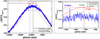 |
Fig. 1 Simulations on influence of Gaussian fitting on piston measurement. |
 |
Fig. 2 Theoretical diagram of differential-scanning piston inversion. |
2.2 Full-link piston-sensing strategy based on differential scanning
Given that the practical segmented imaging system necessitates a piston-monitoring procedure with successive steps from coarse-phasing to fine-phasing control, we established a full-link piston-sensing strategy that employs the proposed differential-scanning piston-inversion theory. The complete workflow of the piston-monitoring procedure is illustrated in Fig. 3.
The entire piston-sensing procedure includes two stages: the coarse-phasing process and the fine-phasing process. In the coarse-phasing process, we began by defining the scanning threshold and step size. The piston modulation is particularly set as an integer multiple of step size (assumed as k times) to simplify the data acquisition. Next, we commanded the piston actuator of the reference segment to traverse within the preset scanning range. After each scan, the focal-plane PSF image was captured and stored in data buffer-1. Once the piston actuator scanned across the threshold, the scanning procedure terminated and an output signal flag was immediately generated, which functions as a command to transfer the captured image sequence from data buffer-1 to the feature-extraction (FE) module for piston inversion. In the FE module, the height of multiple peaks was simultaneously extracted as a feature value utilising the differential scanning piston inversion theory. Specifically, we sequentially extracted the ith and the (i + k)th scanned images from data buffer-1 until the end of sequence and then combined them to form ![Mathematical equation: $\[\frac{2 P_{threshold}}{\Delta p}-k+1\]$](/articles/aa/full_html/2025/07/aa53787-25/aa53787-25-eq21.png) groups of image pairs. Subsequently, through the Fourier transform and differential operation sequentially performed on each image pair, the peak height that characterises the piston of each non-reference segment can be extracted from the resulting differential image, and the
groups of image pairs. Subsequently, through the Fourier transform and differential operation sequentially performed on each image pair, the peak height that characterises the piston of each non-reference segment can be extracted from the resulting differential image, and the ![Mathematical equation: $\[\frac{2 P_{threshold}}{\Delta p}-k+1\]$](/articles/aa/full_html/2025/07/aa53787-25/aa53787-25-eq22.png) rows of feature values ΔMT Fnph–l(l = 1, 2, ..., N) are stored in the preset data buffer-2. To improve the anti-noise capability of the inversion process, several Gaussian functions were applied to fit an optimal response in each column of data buffer-2. Finally, the piston of each non-reference segment can be simultaneously inverted from Eq. (12), and the residual is limited within ±1/2 a wave after the compensation process. At this point, it was ready to start the fine-phasing process. The piston modulation at this stage was set to be within ±1/2 a wave. We first captured the coarse-calibrated PSF and modulated PSF, and then the differential OTF could be calculated by performing the same Fourier transform and differential operation. Through the phase extraction at each peak of differential PTF, the residual piston between the corresponding pair of segments can be exactly inverted using Eq. (15).
rows of feature values ΔMT Fnph–l(l = 1, 2, ..., N) are stored in the preset data buffer-2. To improve the anti-noise capability of the inversion process, several Gaussian functions were applied to fit an optimal response in each column of data buffer-2. Finally, the piston of each non-reference segment can be simultaneously inverted from Eq. (12), and the residual is limited within ±1/2 a wave after the compensation process. At this point, it was ready to start the fine-phasing process. The piston modulation at this stage was set to be within ±1/2 a wave. We first captured the coarse-calibrated PSF and modulated PSF, and then the differential OTF could be calculated by performing the same Fourier transform and differential operation. Through the phase extraction at each peak of differential PTF, the residual piston between the corresponding pair of segments can be exactly inverted using Eq. (15).
Specifically, the sensing range in such a piston-monitoring scheme is not bound by the coherence length, it is only decided by the sweep range covered by the fast steering mirror (FSM). Even when the initial piston is larger than the coherence length of source, it can still be constrained in the diffraction domain through scanning over a large dynamic range. In general, the fulllink piston-sensing procedure is extremely simple to implement, and when the images are taken with the actual image sensor, the problem of non-common path aberrations (NCPA) can be effectively eliminated.
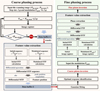 |
Fig. 3 Theoretical diagram of differential-scanning piston inversion. |
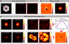 |
Fig. 4 Coarse-phasing-simulation results of JWST-like segmented imaging system. (a) Peak-position extraction. (a1) Configuration of segmented primary mirror with the upper left sub-aperture defined as the reference. (a2) Peak position. (b) Initial state of imaging system before correction. (b1) Initial piston distribution. (b2) Aberrated PSF. (c). Differential spectral-scanning process. The initial PSF and corresponding modulated PSF are shown in (c1) and (c2), the differential MTF and the extracted peak height are shown in (c3) and (c4). (c5) Scanning results and fitted Gaussian function of one non-reference segment. (c6) Residual piston after coarse phasing with average wavefront RMS of 119.8 nm. The corrected PSF and modulated PSF after coarse phasing are shown in (c7) and (c8). The differential MTF and extracted points after coarse phasing are shown in (c9) and (c10). |
3 Simulation results
3.1 Simulation of phasing the JWST-like segmented imaging system
Despite the fact that both the design and construction of JWST have already significantly passed the point of making any further modifications to the hardware or system, this does not necessarily preclude new applications for the existing sensors and mechanisms. A JWST-like segmented imaging system with eighteen 1.32-m-diameter hexagonal sub-mirrors was first simulated to validate the potential of the proposed full-link differentialscanning piston-inversion strategy. The configuration of the segmented primary mirror is illustrated in Fig. 4(a1). Following Eq. (7), the peak position can be jointly determined by the direction and length of the baseline, which is generated by reference and by each non-reference segment, as illustrated in Fig. 4(a2). We set the broadband light source with a central wavelength of 600 nm and a spectral width of 30 nm, which is composed of 11 monochrome lights with an interval of 3 nm. With the uniform spectral-distribution assumption, the coherence length of broadband illumination is defined as (−12μm, 12μm). The equivalent focal length is 100 m, and the pixel size of the detector is 3.45 μm. To simulate the real scene, 1% Gaussian noise (variance σ2 = 1% of that of signal values) was added to each intensity image recorded by the CCD.
We used the upper left segment as the reference and introduced a set of random pistons to the remaining non-reference segment within ±20 μm, as depicted in Fig. 4(b1). Since the differential pistons of some segment pairs exceed the coherence length, the resultant disappearance of the interference fringe leads to a significant blurring of the PSF image, as demonstrated in Fig. 4(b2). Subsequently, we proceeded to implement the differential-scanning piston-sensing procedure. Initially, we commanded the piston position of the reference segment to scan from −40 μm to 40 μm with a step of 20 nm, and the piston modulation was set as 300 nm. After each scanning step, the scanned aberrated image and modulated image were simultaneously recorded, and we were able to calculate the differential OTF. The scanning process is briefly illustrated in Fig. 5. The aberrated images and their corresponding modulated images in the selected scanning step are shown in Figs. 5(a1)–5(f1) and 5(a2)–5(f2), respectively. Within the feature-extraction process, the heights of multiple sets of peaks that characterise the piston of each non-reference segment can be precisely extracted from the calculated differential MTF. It is observable that the peak height associated with each segment exhibit the significant fluctuations due to the piston variation between the reference and non-reference segments, which are shown in Figs. 5(a3)–5(f3) and 5(a4)–5(f4).
The coarse-phasing-simulation results are presented in Figs. 4(c). The aberrated PSF image captured at the initial scanning position and its corresponding modulated image are shown in Figs. 4(c1) and 4(c2), respectively. With the implementation of feature extraction, the lower height, which indicates the larger initial pistons, is simultaneously extracted from the above image pair, as shown in Figs. 4(c3) and 4(c4). Subsequently, through the differential scanning process, the heights of multiple sets of peaks, which characterise the discontinuous wavefront at different scanning steps, can be sequentially recorded. To enhance the inversion accuracy, several Gaussian functions were employed to fit the optimal response to the variations in the heights of the peaks, with one of the fitting results illustrated in Figs. 4(c5) (other fitting results are illustrated in Appendix B, Fig. B.1). Afterwards, the piston of each non-reference segment can be simultaneously inverted, and subsequent compensation results in an average residual wavefront RMS of 119.8 nm are shown in Fig. 4(c6). With coarse phasing done, the 18 segments obviously interfere with each other, generating the high-contrast fringes shown in Fig. 4(c7). Furthermore, the sets of peak height calculated from the coarse calibrated results exhibit a significant enhancement, which is illustrated in Fig. 4(c9) and 4(c10).
The next step was to start the fine-phasing process, for which the piston modulation was set to 30 nm. The initial piston and modulated piston are shown in Figs. 6(a1) and 6(a2), respectively. We first captured the coarse calibrated PSF and modulated PSF, which are illustrated in Figs. 6(a3) and 6(a4); subsequently, we were able to obtain the differential OTF. Through the phase extraction at each peak position of differential PTF, the residual piston can be exactly inverted, as shown in Fig. 6(a5). Finally, the interference pattern generated by fine phasing is distributed symmetrically, with an obvious peak centred. The average residual wavefront RMS is 0.035 waves at the 600 nm central wavelength.
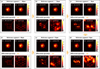 |
Fig. 5 Peak-height extraction-process simulation results of JWST-like segmented imaging system. Samples of (a1)–(f1) aberrated PSFs and (a2)–(f2) modulated PSFs captured during scanning. (a3)–(f3) Differential MTFs calculated by Fourier transformer and differential operation. (a4)–(f4) Extracted peak heights that characterise the pistons of all non-reference segments. |
3.2 Simulation of phasing a 126-unit segmented imaging system
Future astronomical observation missions necessitate extremely large aperture telescopes with hundreds of segments to attain milliarcsecond-angular-resolution capability. In this section, we describe how we simulated a segmented imaging system made of 126 units, and we consider the future applicability of the proposed piston-sensing strategy. The segment arrangement is illustrated in Fig. 7(a1). With the upper left sub-aperture defined as the reference, the multiple peak positions that characterise each non-reference segment’s piston can be acquired from Eq. (9), as shown in Fig. 7(a2). Similarly, 1% Gaussian noise was also added to simulate the real observation scene. The equivalent focal length is 300 m, and the pixel size of the detector is 3.45 μm. Since the broadband illumination parameters are consistent with those in Sect. 3.1, the coherence length of the light source was maintained at (−12 μm, 12 μm), and the initial piston of each non-reference segment was also set to the displacement within ±20 μm. The initial piston distribution and the aberrated PSF image are illustrated in Figs. 7(b1) and 7(b2), respectively.
The piston modulation for the coarse-phasing stage and fine-phasing stage are still set as 300 nm and 30 nm, respectively. In the differential spectral-scanning process, the piston actuator of the reference segment was first set to scan from −40 μm to 40 μm with a step of 20 nm. At each scanning step, the heights of multiple sets of peaks that characterise the piston variation of each non-reference segment can be extracted from the differential MTF. The aberrated PSF image and corresponding modulated image which were taken at the initial position of the scan are shown in Figs. 7(c1) and 7(c2), respectively. The differential MTF and the secondary-peak intensity are illustrated in Figs. 7(c3) and 7(c4), respectively. It can be seen that the large initial pistons cause the height of each peak to almost be drowned out by the noise. When the scanning was complete, several Gaussian functions were simultaneously used to fit the optimal response to the variations in the heights of the peaks, with one of the fitting curves shown in Fig. 7(c5). Through the final inversion and compensation process, the differential piston of each non-reference segment was retrieved from the fitted results, and the residual piston is illustrated in Fig. 7(c6), where the average residual wavefront RMS is 127.2 nm. The corrected PSF image and its corresponding modulated image are shown in Figs. 7(c7) and 7(c8), respectively, which appear with a faintly visible main peak and an approximately symmetric interference pattern. Furthermore, by comparing with the differential MTF before and after correction, the significant improvement in secondary-peak intensity further demonstrates the effective calibration of discontinuous wavefront, as illustrated in Figs. 7(c9) and 7(c10).
The fine-phasing process follows immediately after the coarse scanning, and the correction results are shown in Fig. 8. The initial piston after coarse calibration and its modulated piston are illustrated in Figs. 8(a1) and 8(a2), respectively. By performing the differential spectral analysis on the coarse calibrated PSF and its modulated PSF, the pistons limited to within ±1/2 a wave can be simultaneously extracted from the calculated differential PTF, as shown in Fig. 8(a5). Fine phasing ensures the interference pattern is distributed symmetrically, with an obvious peak centred; and the average residual wavefront RMS is 32.3 nm, which is merely one-tenth of the wavelength, as illustrated in Figs. 8(b1) and 8(b2).
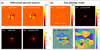 |
Fig. 6 Fine-phasing-simulation results of JWST-like segmented imaging system. (a) Differential-spectral-analysis process. The initial piston distribution and modulated piston distribution are shown in (a1) and (a2). The corresponding initial aberrated PSF and modulated PSF are shown in (a3) and (a4). (a5) Differential PTF. (b) Fine-phasing results. The residual piston and corrected PSF with wavefront RMS of 21.4 nm are shown in (b1) and (b2). |
3.3 Analysis of factors affecting piston-sensing accuracy
In contrast to the conventional dOTF technique, our proposed method significantly extends the detection range beyond the single-wavelength limit through continuous piston modulation. However, the time required for the process, combined with the integration time needed to achieve a good signal-to-noise ratio (S/N), results in a significant limitation to its practical applicability. Specifically, as the number of segments increases, the differential MTF signal under the rated integration time will be submerged by other noise contributions, which will cause the deviations of the optimal response position. Moreover, the additional phase variations introduced by continuous modulation can disrupt the OTF subtraction procedure, resulting in residual errors that may overshadow the differential MTF signal. Finally, although tip-tilt correction can mitigate the line-of-sight disturbances, the effect of residuals on the proposed method also requires quantitative analysis. Consequently, to systematically evaluate the piston-sensing performance of the proposed method, this section presents a comprehensive analysis via numerical simulations, investigating its robustness under different noise levels, tip-tilt residuals, and phase variations.
3.3.1 Discussion on the influence of different noise levels
According to the theoretical derivation in Sect. 2, the noise of the image plane may degrade the accuracy of piston inversion. Although Gaussian fitting can improve the anti-noise ability of the coarse-phase process, the random noise distribution probably shifts the optimal response position in the peak height variation, which causes the coarse-calibrated residual out of one wavelength. Additionally, the decline of coarse-phasing accuracy will directly lead to the 2π ambiguity in the subsequent fine-phasing check, and the random phase of image noise also inevitably causes the extraction deviation of differential phase. Consequently, through lots of simulation experiments, we analysed the performance of the proposed piston inversion theory under different noise levels and further bridge the gap between the theory and future system-level applications.
We used a JWST-like segmented arrangement to evaluate the piston inversion performance under different noise levels (variance σ2 = 3%, 5%, 7%, 10%). The simulation parameters–including spectral distribution, scanning range, and modulation amount– are consistent with those described in Sect. 3.1, and simulation results are presented in Fig. 9. We can see that as the noise level increases, the RMS of the residual wavefront after the coarse-phasing stage remains almost within 1/4 of a wave and does not exhibit an evident decreasing trend. The stable piston residuals demonstrate that the Gaussian fitting process can not only effectively reduce the influence of noise fluctuation on the optimal response extraction, it can also avoid the 2π ambiguity in the subsequent fine-phasing check. Additionally, with the increase of the noise level, the random phase further affects the differential phase extraction, resulting in a gradual decline in accuracy. However, even if 10% Gaussian noise is added to the intensity image, the RMS of the wavefront residual after inversion is still within 0.05 wavelengths. Consequently, according to these simulation results, it is concluded that the full-link phasing strategy based on the differential-scanning piston-inversion theory demonstrates remarkable robustness when faced with image noise.
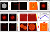 |
Fig. 7 Coarse-phasing simulation results of 126-unit segmented-imaging system. (a) Peak-position extraction. (a1) Configuration of segmented primary mirror with the upper left sub-aperture defined as the reference. (a2) Peak position. (b) Initial state of imaging system before correction. (b1) Initial piston distribution. (b2) Aberrated PSF. (c). Differential spectral-scanning process. The initial PSF and corresponding modulated PSF are shown in (c1) and (c2). The differential MTF and extracted peaks are shown in (c3) and (c4). (c5) Scanning results and fitted Gaussian function of one non-reference segment. (c6) Residual piston after coarse phasing with an average wavefront RMS of 127.2 nm. The corrected PSF and modulated PSF after coarse phasing are shown in (c7) and (c8). The differential MTF and extracted points after coarse phasing are shown in (c9) and (c10). |
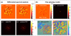 |
Fig. 8 Fine-phasing simulation results of 126-unit segmented-imaging system. (a) Differential spectral-analysis process. The initial piston distribution and modulated piston distribution are shown in (a1) and (a2). The corresponding initial aberrated PSF and modulated PSF are shown in (a3) and (a4). (a5) Differential PTF. (b) Fine-phasing results. Residual piston and corrected PSF with wavefront RMS of 32.3 nm are shown in (b1) and (b2). |
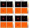 |
Fig. 9 Piston-inversion performance under different noise levels. (a1)–(d1) Coarse-phased PSFs. (a2)–(d2) Fine-phased PSFs. (a3)–(d3) Coarse-phased residuals with stable wavefront RMS within one wavelength. (a4)–(d4) Fine-phased residuals with gradually declined wavefront RMS within 0.05 wavelengths. |
3.3.2 Discussion on the influence of different tip-tilt errors
To analyse the effect quantitatively, we explored the impact of tip-tilt errors on the piston-sensing performance in a JWST-like segmented system, which also has the same configuration as described in Sect. 3.1. According to the Nyquist sampling law, the pixel size of a scientific imaging camera must be smaller than the diffraction limit of the system for accurate imaging. Since previous work (Carlisle & Acton 2015) indicate that the measurement of pistons requires a stacking error of less than half a pixel, we designed simulations with tip-tilt errors ranging from 0.5 to 2 times the diffraction limit. In each set of simulations, random tip-tilt errors within a specified range are loaded in each modulation step, and the piston-sensing results are presented in Fig. 10. Based on the simulation parameters, the diffraction limit of the JWST-like segmented system is determined to be 0.112 μrad. During the coarse-phasing process for each set of simulation, the scanning results of peak height are illustrated in Figs. 10(a3) and 9,(d3) respectively. The differential piston of each non-reference segment can be simultaneously inverted from the scanning curve by Gaussian fitting. The coarse-phased PSF images and their corresponding residuals are shown in Figs. 10(a1)–9(d1) and Figs. 10(a2)–9(d2), respectively. Notably, despite the fact that the height of the peak will gradually become noisier with the increase of tip-tilt error, the Gaussian fitting process can still effectively extract the optimal response position, maintaining the RMS of the residual wavefront within 1/2 a wave after the coarse-phasing stage. However, the tip-tilt error will directly influence the phase distribution in the differential PTF, thus significantly affecting the fine-phase process. Compared to the RMS in ideal conditions without tip-tilt errors, there is no evident deterioration in sensing accuracy in cases with tip-tilt errors within the diffraction limit. The fine-phased PSF images are shown in Figs. 10(a4) and 10(b4), and the residuals are shown in Figs. 10(a5) and 10(b5), respectively. When the tip-tilt errors are 1.5 times the diffraction limit or more, the RMS of the wavefront residual after inversion is beyond 0.1λ. Consequently, to ensure the piston-sensing accuracy, the tip-tilt error of each segment must be calibrated within the diffraction limit.
3.3.3 Discussion on the influence of different phase variations
In practical applications, the broader disturbances, such as turbulence and primary mirror vibrations, will introduce random phase fluctuations in each modulated OTF and subsequently bring residual errors that may overshadow the differential MTF signal. Particularly, more time-varying fluctuations inevitably occur during the continuous modulation process. Shortening the exposure time to fall within the timescale of these fluctuations appears to be an effective approach to mitigating temporal phase variations. However, as the number of segments increases, the decreasing relative size between the modulated segment and the monolithic primary mirror will lead to a degradation in the SNR of the differential MTF, in which case sacrificing the exposure time is no longer acceptable. Specifically, a comparison between Fig. 4(c5) and Fig. 7(c5) reveals that the differential MTF signal for 126 segments becomes significantly noisier. Consequently, high-quality differential signal measurement requires a sufficient number of photons in each PSF exposure, enabling the differential MTF signal to dominate other noise contributions. Obviously, more severe conflict arises in configurations with numerous segments: a longer exposure time brings larger phase variations, whereas a shorter exposure time causes a lower SNR. Integrating the effects of the mentioned factors is crucial for identifying the applicable boundary of this method. In this section, through the numerical simulations, we analyse how different phase variations affect piston-sensing accuracy under varying SNRs and discuss its potential impact on the feasibility of the proposed method.
We used a 126-unit segmented arrangement to evaluate the piston-sensing performance under different noise levels and different phase variations. The simulation parameters are consistent with those described in Section 3.1. First, we designed three sets of simulations under different noise levels (variance σ2 = 1%, 5%, 10%). Then, in each set of simulations, we set four different phase-variation amplitudes. In each scanning step of the continuous modulation, random phase errors within the corresponding amplitude range are loaded to each segment to simulate a real-world application. Specifically, the scanning step size in the coarse-phasing process changes from a constant Δp to a variable Δp + pϵ, and the phase modulation in the fine-phasing stage changes from a constant Δφ to ![Mathematical equation: $\[\Delta \varphi+\frac{2 \pi p_{\epsilon}}{\lambda_{mid}}\]$](/articles/aa/full_html/2025/07/aa53787-25/aa53787-25-eq23.png) , where pϵ represents the piston modulation error corresponding to the random phase variation. The simulation results are shown in Figs. 11–13. Within the same noise variance, as the amplitude of phase variations increases, the scanning curves of the secondary peak heights all become noisier, and the piston inversion accuracy also gradually decreases. It can be seen that when the noise variance is 1%, random phase variations within the range of 100 nm do not affect the coarse-phasing accuracy, as illustrated in Fig. 11. When the noise variance reaches 5%, random phase variations exceeding 100 nm do indeed degrade the coarse-phasing accuracy of certain segments to levels surpassing 1/2 a wave. However, it is noteworthy that the residuals observed in this scenario are larger compared to those occurring when the noise variance is at 1%, as clearly depicted in Fig. 12. When the noise variance is increased to 10%, we adjusted the amplitudes of the phase variations to 200 nm, 100 nm, 50 nm, and 20 nm, considering that shorter exposure times correspond to smaller phase variations. The simulation results reveal that there is no notable adverse effect on coarse phasing accuracy only when the phase variation is controlled to within 20 nm, as illustrated in Fig. 13. However, it seems that the fine-phasing procedure rarely fails to work in the same conditions. The RMS result close to 0.1λ is achieved only when the phase variations are within [−20 nm, 20 nm], as shown in Fig. 13(d). In this case, residual pistons for most of the segments are fine-phased, even though several of them remain at about 300 nm, which suggests that fine phasing may be available in a more stable environment.
, where pϵ represents the piston modulation error corresponding to the random phase variation. The simulation results are shown in Figs. 11–13. Within the same noise variance, as the amplitude of phase variations increases, the scanning curves of the secondary peak heights all become noisier, and the piston inversion accuracy also gradually decreases. It can be seen that when the noise variance is 1%, random phase variations within the range of 100 nm do not affect the coarse-phasing accuracy, as illustrated in Fig. 11. When the noise variance reaches 5%, random phase variations exceeding 100 nm do indeed degrade the coarse-phasing accuracy of certain segments to levels surpassing 1/2 a wave. However, it is noteworthy that the residuals observed in this scenario are larger compared to those occurring when the noise variance is at 1%, as clearly depicted in Fig. 12. When the noise variance is increased to 10%, we adjusted the amplitudes of the phase variations to 200 nm, 100 nm, 50 nm, and 20 nm, considering that shorter exposure times correspond to smaller phase variations. The simulation results reveal that there is no notable adverse effect on coarse phasing accuracy only when the phase variation is controlled to within 20 nm, as illustrated in Fig. 13. However, it seems that the fine-phasing procedure rarely fails to work in the same conditions. The RMS result close to 0.1λ is achieved only when the phase variations are within [−20 nm, 20 nm], as shown in Fig. 13(d). In this case, residual pistons for most of the segments are fine-phased, even though several of them remain at about 300 nm, which suggests that fine phasing may be available in a more stable environment.
In summary, although longer exposure times required for a high SNR may lead to larger phase fluctuations, the coarse-phasing procedure can still attain high-precision piston measurements when the phase variation is limited within a certain range. Nonetheless, as the external disturbances intensify, the extreme phase variation may completely overshadow the differential MTF signal. At this point, increasing exposure times can no longer offset the decline in accuracy caused by phase fluctuations. Consequently, the real-world application for coarse phasing demands an optimal trade-off between the higher SNR and the slighter temporal phase variation. The following fine-phasing procedure brings stricter requirements for the application environment, especially with an even slighter phase variation.
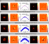 |
Fig. 10 Simulation on influence of tip-tilt errors. (a1)–(d1) Coarse-phased PSF, (a2)–(d2) coarse-phased residual piston, (a3)–(d3) scanning results, (a4)–(d4) fine-phased PSF, and (a5)–(d5) fine-phased residual piston, for four cases corresponding to 0.5, 1.0, 1.5, and 2.0 times the diffraction limit. |
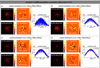 |
Fig. 11 Simulations on influence of different phase variations with noise σ2 = 1% on full-link piston sensing. (a) Analysis of different phase variations within [−500 nm, 500 nm]. (b) Analysis of different phase variations within [−300 nm, 300 nm]. (c) Analysis of different phase variations within [−100 nm, 100 nm]. (d) Analysis of different phase variations within [−50 nm, 50 nm]. |
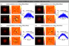 |
Fig. 12 Simulations on influence of different phase variations with noise σ2 = 5% on full-link piston sensing. (a) Analysis of different phase variations within [−500 nm, 500 nm]. (b) Analysis of different phase variations within [−300 nm, 300 nm]. (c) Analysis of different phase variations within [−100 nm, 100 nm]. (d) Analysis of different phase variations within [−50 nm, 50 nm]. |
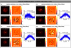 |
Fig. 13 Simulations on influence of different phase variations with noise σ2 = 10% on full-link piston sensing. (a) Analysis of different phase variations within [−200 nm, 200 nm]. (b) Analysis of different phase variations within [−100 nm, 100 nm]. (c) Analysis of different phase variations within [−50 nm, 50 nm]. (d) Analysis of different phase variations within [−20 nm, 20 nm]. |
3.3.4 Discussion on the combined effects of tip-tilt errors and phase variations
Based on the preceding simulation analysis, it is apparent that the proposed method is indeed influenced by tip-tilt errors and time-varying phase variations, with these effects becoming particularly significant during the fine-phasing stage. Moreover, in a real-world scenario, it is essential to acknowledge that these factors do not occur in isolation; rather, they typically manifest concurrently and exert a combined influence on the performance of the proposed method. To address this complexity and gain a more comprehensive analysis of the method’s behaviour under realistic conditions, in this section, we outline additional simulations that accurately combine the effects of tip-tilt errors and phase variations.
The simulation platform and parameter settings are consistent with the 126-unit segmented system of Sect. 3.2. Drawing on the specified simulation parameters, the diffraction limit of the system is determined to be 0.043 μrad. Given that large time-varying phase variations and tip-tilt errors can render the fine-phasing process ineffective, this section focuses exclusively on combinations of phase-variation thresholds of 20 nm and 50 nm, alongside tilt-error thresholds of 0.043 μrad and 0.065 μrad. The simulation results are shown in Fig. 14. When the tip-tilt error and time-varying phase error are limited to within 0.043 μrad and 20 nm, respectively, both the coarse-phasing and fine-phasing processes can be successfully executed simultaneously. However, in the case where the tiptilt error increases to 0.043 μrad or the phase error increases to 50 nm, the fine-phasing process completely fails to work, although the coarse-phasing process exhibits notable robustness with extremely high correction accuracy.
In conclusion, although the simulation results indicate the potential for implementing the full-link piston sensing procedure, its practical application is subject to limitations due to the complex phase variations and tip-tilt errors. Specifically, the applicable boundaries of the coarse- and fine-phasing steps are distinct, with the fine-phasing process exhibiting greater sensitivity to phase perturbations compared to the coarse-phasing process. Furthermore, if the phase fluctuations are slight, the acquired data calculated from the fine-phasing domain could potentially assist us in evaluating the piston and tip-tilt simultaneously, which also offers a possible way to mitigate the impact of tip-tilt.
4 Experimental results
To further validate the practical applicability of the proposed method, an optical desktop experiment is implemented in a simplified seven-unit segmented imaging setup, as shown in Fig. 15. In the experiment, we used a supercontinuum laser (NKT EX-20) and a collimator to provide the parallel broadband illumination of which the wavelength ranges from 550 nm to 650 nm. The FSM array serving as a piston compensator is composed of eight piezoelectric fast steering mirrors (FSM, P32.ZT4S), arranged in a circular ring with an outer diameter of 90 mm. Upon applying a voltage to the actuator, the FSM generates piston motion, thus introducing a piston error in the light beam reflected by the corresponding segment. Limited by the experimental devices, segments 1, 2, 3, 4, 5, 6, and 7 were chosen for the experiment, with each segment having a diameter of 15 mm. Since segment 5 was set as the reference, the resultant three pairs of redundant baselines (5–3 and 7–1, 5–6 and 2–1, 5–7 and 3–1) will cause an intricate entanglement among the piston characteristics of the corresponding segment, as depicted in the upper right corner of Fig. 11. Being sequentially reflected by the flat mirror and the piston compensator placed at a 45° angle, the parallel light is split into seven beams and then concentrated by using a lens with 2 m focal length. To evaluate the accuracy of the piston calibration, a beam splitter (BS) was used to split the converging beam into two separate light beams. In the transmission path, the light beam is directly captured by a phasing camera. In the reflection path, a filter wheel is placed in front of the calibration camera. When we rotate the filter wheel, the polychromatic light can be transformed to specific monochromatic light by different filters. The piston calibration is considered complete, provided that the PSF image in the calibration camera remains stable despite variations in the filter. The pixel size of the imaging camera and calibrated camera are both 3.45 μm (STC-SPB322PCL).
Next we performed the full-link piston sensing procedure on the simplified segmented-imaging setup, and the entire experimental results are presented in Fig. 16. At the beginning, the broadband PSF image without piston aberration should be obtained after the system calibration. Since the piston compensator is placed at 45 degrees, the actual piston application is ![Mathematical equation: $\[\sqrt{2}\]$](/articles/aa/full_html/2025/07/aa53787-25/aa53787-25-eq24.png) times that loaded by the FSM. The coarse-phasing process is then started, and the piston modulation amount is set to 235.6 nm in this process. After loading a specific set of pistons into all non-reference segments, the aberrated PSF in initial state and its modulated image are illustrated in Figs. 16(a1) and 16(a2), respectively. Through the differential operation, it can be seen that the initial secondary-peak intensity is almost submerged in the noise distribution, as illustrated in Figs. 16(a3) and 16(a4). Next, we set the FSM that corresponds to the reference segment to scan from −11 783 nm to 11 783 nm with a step size of 11.78 nm, and the PSF images captured after each step were sequentially stored in the preset data-buffer 1. Upon completion of the scanning, with the modulation amount defined as 20 times the step size, 1981 groups of image pairs were formed by sequentially extracting two images labelled i and i + 20 from data-buffer 1 and subsequently transmitted to the FE module to calculate the piston-response peak height of each non-reference segment. Afterwards, the optimal response identification was achieved via a Gaussian fitting of the six groups of peak height variation, and the scanning data and fitting curves are illustrated in Fig. 16(a5). After completing the final inversion and compensation process, the differential piston of each non-reference segment can be retrieved from the fitted results, and the average residual wavefront RMS is 0.18λ, which is within one wavelength. The pistons measured by the coarse-phasing process are simultaneously compensated to the corresponding non-reference segment before the fine-phasing process. The coarse-calibrated PSF and its modulated image, exhibiting a faintly visible main peak and an approximately symmetric interference pattern, are illustrated in Figs. 16(a6) and 16(a7), respectively. Furthermore, compared with the initial state, the sets of secondary-peak intensities calculated from the coarse-calibrated results exhibit a significant enhancement, which is illustrated in Figs. 16(a8) and 16(a9). The fine-phasing process follows immediately after the coarse calibration, where the initial PSF is exactly the image corrected by coarse phasing, as shown in Fig. 16(b1). With an identical piston modulation amount of 235.6 nm, the residual pistons of each non-reference segment can be simultaneously extracted from the calculated differential PTF, as shown in Fig. 16(b2).
times that loaded by the FSM. The coarse-phasing process is then started, and the piston modulation amount is set to 235.6 nm in this process. After loading a specific set of pistons into all non-reference segments, the aberrated PSF in initial state and its modulated image are illustrated in Figs. 16(a1) and 16(a2), respectively. Through the differential operation, it can be seen that the initial secondary-peak intensity is almost submerged in the noise distribution, as illustrated in Figs. 16(a3) and 16(a4). Next, we set the FSM that corresponds to the reference segment to scan from −11 783 nm to 11 783 nm with a step size of 11.78 nm, and the PSF images captured after each step were sequentially stored in the preset data-buffer 1. Upon completion of the scanning, with the modulation amount defined as 20 times the step size, 1981 groups of image pairs were formed by sequentially extracting two images labelled i and i + 20 from data-buffer 1 and subsequently transmitted to the FE module to calculate the piston-response peak height of each non-reference segment. Afterwards, the optimal response identification was achieved via a Gaussian fitting of the six groups of peak height variation, and the scanning data and fitting curves are illustrated in Fig. 16(a5). After completing the final inversion and compensation process, the differential piston of each non-reference segment can be retrieved from the fitted results, and the average residual wavefront RMS is 0.18λ, which is within one wavelength. The pistons measured by the coarse-phasing process are simultaneously compensated to the corresponding non-reference segment before the fine-phasing process. The coarse-calibrated PSF and its modulated image, exhibiting a faintly visible main peak and an approximately symmetric interference pattern, are illustrated in Figs. 16(a6) and 16(a7), respectively. Furthermore, compared with the initial state, the sets of secondary-peak intensities calculated from the coarse-calibrated results exhibit a significant enhancement, which is illustrated in Figs. 16(a8) and 16(a9). The fine-phasing process follows immediately after the coarse calibration, where the initial PSF is exactly the image corrected by coarse phasing, as shown in Fig. 16(b1). With an identical piston modulation amount of 235.6 nm, the residual pistons of each non-reference segment can be simultaneously extracted from the calculated differential PTF, as shown in Fig. 16(b2).
Finally, the interference pattern corrected by fine phasing is distributed symmetrically with an obvious centred peak, which is illustrated in Fig. 16(b3). After the full-link phasing process, the average residual wavefront RMS is 0.05 waves at the 600 nm central wavelength, as detailed in Table 1.
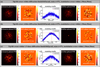 |
Fig. 14 Simulations on influence of combined effects of tip-tilt errors and phase variations. (a) Tip-tilt errors within diffraction limit; noise σ2 = 5%; phase variations within [−50 nm, 50 nm]. (b) Tip-tilt errors within diffraction limit; noise σ2 = 5%; phase variations within [−20 nm, 20 nm]. (c) Tip-tilt errors within 1.5 times the diffraction limit; noise σ2 = 5%; phase variations within [−20 nm, 20 nm]. |
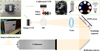 |
Fig. 15 Simplified seven-unit optical desktop experimental setup. |
Residual piston of each non-reference segment in different correction stages.
5 Conclusions
Future extremely large segmented telescopes strictly rely on a continuous piston-monitoring procedure to realise diffraction-limited resolution equivalent to that of a single aperture. Unfortunately, existing methods are always challenged by the trade-off among detection range, accuracy, and segment number, preventing the attainment of diffraction-limited resolution from real-world instruments. In this work, we innovatively derived a differential-scanning piston-inversion theory, which not only significantly mitigates the intrinsic constraint of piston characterisation caused by redundant baselines, it also makes up for the detection range shortfall of former optical differential models in segmented co-phasing. By performing the large-scale piston scanning of the reference segment and applying continuous differential operations, the secondary-peak overlap resulting from the redundant baselines can be completely eliminated, while a differential MTF sequence that exclusively encapsulates the piston information of each non-reference segment can be simultaneously constructed. Afterwards, the multi-point information in the differential MTF image was sampled to compose the feature vector that can precisely respond to the piston variation. To address the inevitable issue of imaging noise, multiple sets of Gaussian functions were employed to approximate the optimal response positions within the variations of secondary-peak intensity. Through the integration of the fitting results and derived error-inversion conclusions, the coarse calibration of each non-reference segment piston can be effectively realised. Finally, following the immediate application of secondary piston modulation and differential operation, the phase information of each non-reference segment was extracted through the differential spectrum analysis, thereby enabling the precise piston alignment within the diffraction domain.
Based on the proposed theoretical model, we also devised a full-link piston-sensing strategy, intended to serve as a technical reserve for future high-resolution astronomical observations. On the one hand, the practical implementation of this strategy enables simultaneous piston extraction, which is directly based on the PSF images captured by scientific imaging cameras. Since the proposed method eliminates the need for the construction of complex beam splitting pathways, the potentially introduced and recalcitrant no-common-path aberrations that may arise from such pathways can be effectively circumvented. On the other hand, the detection range of the proposed piston-sensing scheme is independent of the coherence length restrictions and only relies on the boundaries of the FSM capture range. This means that the availability of such a scheme will provide some level of mission risk reduction and can be used to double check other co-phasing procedure results as needed.
Both simulation and experimental results demonstrate the potential of the proposed strategy on full-link piston sensing. However, non-negligible constraints on its applicability persist in practical scenarios due to time-varying phase errors and tiptilt errors. The successful implementation of this strategy may necessitate additional components to control these errors within acceptable thresholds. Furthermore, its effectiveness needs to be rigorously validated under realistic conditions, especially given the uncertainties surrounding the stability and operational conditions of future extremely large segmented telescopes such as the ELTs. It is also critical to note that certain applications require fine-phasing residuals of 10 nm or lower levels not currently achieved by the presented method. In conclusion, while meaningful progress has been made, substantial work remains to be done to address these limitations, thereby enabling the proposed method to find wider applications in future extremely large segmented-aperture telescopes.
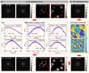 |
Fig. 16 Optical desktop experimental results. (a) Coarse-phasing process. The initial PSF and corresponding modulated PSF are shown in (a1) and (a2). The differential MTF and extracted feature points are shown in (a3) and (a4). The scanning results and fitted Gaussian functions of six non-reference segments are shown in (a5). The corrected PSF and modulated PSF after coarse phasing are shown in (a6) and (a7). The differential MTF and the extracted height of peak after coarse phasing are shown in (a8) and (a9). (b) Fine-phasing process. (b1) Initial PSF before fine phasing. (b2) Phase-extracted from differential PTF. (b3) Corrected PSF after fine phasing. |
Acknowledgements
This work was supported by the National Key Research and Development Program of China (2022YFB3901900), National Natural Science Foundation of China (62175243) and Youth Innovation Promotion Association, CAS (2020372).
Appendix A Coarse phasing of the extended scene
When segmented telescopes observe the extended scenes with complex structures, the spatial properties of the target and the PSF will undergo convolution effects on the scientific image plane, posing a significant challenge to numerous existing point-source piston sensing methods. Although the precise calibration can be accomplished through the utilization of beacon sources, including bright stars or artificial guide stars, the extended target piston sensing techniques are still considered to be a particularly promising option due to their robust adaptability. In practice, the proposed differential scanning piston inversion theory is also applicable to the coarse phasing of the extended scene. Based on the Fourier optics, the image captured in the scientific image plane can be expressed as the convolution between the extended target and the PSF of segmented system:
![Mathematical equation: $\[I(x, y)=\frac{\Delta \lambda}{M} \sum_{i=1}^M O_{\lambda_i}(x, y) \otimes \operatorname{PSF}_N\left(x, y, \lambda_i\right),\]$](/articles/aa/full_html/2025/07/aa53787-25/aa53787-25-eq25.png) (A.1)
(A.1)
where Oλi(x, y) represents the intensity distribution of observation and ⊗ is the convolution notation. Under the gray-world approximation, the captured image can be simplified as:
![Mathematical equation: $\[I(x, y)=O(x, y) \otimes \operatorname{PSF}_N(x, y).\]$](/articles/aa/full_html/2025/07/aa53787-25/aa53787-25-eq26.png) (A.2)
(A.2)
Substituting the above equation into the derivation of Sect 2.1, the differential MTF that contains the peak height of each non-reference segment can be expressed as:
![Mathematical equation: $\[\Delta M T ~F_{\text {ext-s }}=|F\{O\}| \cdot \Delta M T ~F_{\mathrm{s}}.\]$](/articles/aa/full_html/2025/07/aa53787-25/aa53787-25-eq27.png) (A.3)
(A.3)
Then the height of each peak is extracted as:
![Mathematical equation: $\[\begin{aligned}& \Delta M T ~F_{n p h-l}=\left|F\left\{O\left(\frac{B_{\mu_{1 l}}}{\lambda_{\operatorname{mid}} f}, \frac{B_{\nu_{1 l}}}{\lambda_{\operatorname{mid}} f}\right)\right\}\right| \cdot \Delta M T ~F_{\mathrm{s}}\left(\frac{B_{\mu_{1 l}}}{\lambda_{\operatorname{mid}} f}, \frac{B_{\nu_{1 l}}}{\lambda_{\operatorname{mid}} f}\right) \\& \quad=\kappa_{1 l} \cdot \Delta M T ~F_{\mathrm{s}}\left(\frac{B_{\mu_{1 l}}}{\lambda_{\operatorname{mid}} f}, \frac{B_{\nu_{1 l}}}{\lambda_{\operatorname{mid}} f}\right) \\& \text { s.t. } l=2,3, \ldots, N.\end{aligned}\]$](/articles/aa/full_html/2025/07/aa53787-25/aa53787-25-eq28.png) (A.4)
(A.4)
Since we assume that the observation scene is stationary, the spatial frequency information of the target at each secondary-peak position can be regarded as a constant κ1l. In this case, the coarse piston inversion theory derived in this paper is also applicable to the extended target.
We still utilize a JWST-like segmented arrangement to evaluate the coarse piston inversion performance in the extended scene. We use the real extended scene, namely “The pillars of Creation”, which is captured by James Webb Space Telescope’s Near-Infrared Camera (NIRcam), to simulate the piston inversion process and the simulation results are shown in Fig. A.1. The initial piston and aberrated image are respectively illustrated in Fig. A.1(a1) and A.1(a2). With the implementation of feature extraction, the lower height of peak which indicate the larger initial pistons are extracted from the differential MTF, as shown in Fig. A.1(a3) and A.1(a4). Through the differential scanning coarse phasing process, the piston of each non-reference segment can be simultaneously inverted, and subsequent compensation results in an average residual wavefront RMS of 0.124 μm, as shown in Fig. A.1(b2). It can be seen that both the contrast of the corrected image and the sets of peak heights calculated from the coarse calibrated results exhibit a significant enhancement, which are illustrated in Fig. A.1(b1), A.1(b3) and A.1(b4). Compared to the initial state, the frequency response of imaging system is also greatly improved as shown in Fig. A.1(a5) and A.1(b5).
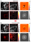 |
Fig. A.1 Extended scene coarse phasing simulation results of JWST-like segmented imaging system. (a). Initial state. The initial degraded image and loaded piston distribution are respectively shown in (a1) and (a2), differential MTF and extracted heights of peak are shown in (a3) and (a4). The degraded MTF is illustrated in (a5). (b). Corrected results. The corrected image, differential MTF, extracted heights of peak and the corrected MTF are respectively shown in (b1), (b3), (b4), and (b5). (b2) residual piston after coarse phasing with average wavefront RMS of 124 nm. |
Appendix B The Gaussian fitting results in the coarse phasing simulation process
Simultaneously utilizing several Gaussian functions to model the optimal responses of multiple sets of secondary-peaks intensity, the piston of each non-reference segment can be retrieved from the final inversion process. The variations and Gaussian fitting results of each peak height are illustrated in Fig. B.1, providing a clear visualization of the data.
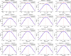 |
Fig. B.1 The variation and Gaussian fitting result of peak height in the coarse phasing simulation process of JWST-like imaging system. |
References
- Acton, D. S., Towell, T., Schwenker, J., et al. 2007, in Proceedings of SPIE, 6687, UV/Optical/IR Space Telescopes: Innovative Technologies and Concepts III, eds. H. MacEwen & J. Breckinridge, SPIE, conference on UV/Optical/IR Space Telescopes: Innovative Technologies and Concepts III, San Diego, CA, August 26–29, 2007 [Google Scholar]
- Acton, D. S., Knight, S., Carrasquilla, M., et al. 2022, in Proceedings of SPIE, 12180, Space Telescopes and Instrumentation 2022: Optical, Infrared, and Millimeter Wave, eds. L. Coyle, S. Matsuura, & M. Perrin, SPIE, conference on Space Telescopes and Instrumentation – Optical, Infrared, and Millimeter Wave, Montreal, Canada, July 17–22, 2022 [Google Scholar]
- Bertrou-Cantou, A., Gendron, E., Rousset, G., et al. 2022, A&A, 658, A49 [NASA ADS] [CrossRef] [EDP Sciences] [Google Scholar]
- Bolcar, M. R., & Fienup, J. R. 2009, Appl. Opt., 48, A5 [Google Scholar]
- Carlisle, R. E., & Acton, D. S. 2015, Appl. Opt., 54, 6454 [Google Scholar]
- Chanan, G., Troy, M., Dekens, F., et al. 1998, Appl. Opt., 37, 140 [NASA ADS] [CrossRef] [Google Scholar]
- Chanan, G., Ohara, C., & Troy, M. 2000a, Appl. Opt., 39, 4706 [NASA ADS] [CrossRef] [Google Scholar]
- Chanan, G. A., Troy, M., & Ohara, C. M. 2000b, in Optical Design, Materials, Fabrication, and Maintenance, 4003, ed. P. Dierickx, International Society for Optics and Photonics (SPIE), 188 [Google Scholar]
- Codona, J. L., & Doble, N. 2015, J. Astron. Telesc. Instrum. Syst., 1 [Google Scholar]
- Crooke, J. A., Roberge, A., Domagal-Goldman, S. D., et al. 2016, in Proceedings of SPIE, 9904, Space Telescopes and Instrumentation 2016: Optical, Infrared, and Millimeter Wave, eds. H. MacEwen, G. Fazio, & M. Lystrup, SPIE, conference on Space Telescopes and Instrumentation – Optical, Infrared, and Millimeter Wave, Edinburgh, Scotland, June 26-July 01, 2016 [Google Scholar]
- France, K., Tumlinson, J., Fleming, B., et al. 2024, J. Astron. Telesc. Instrum. Syst., 10 [Google Scholar]
- Gonsalves, R. A., & Chidlaw, R. 1979, in Applications of Digital Image Processing III, 0207, ed. A. G. Tescher, International Society for Optics and Photonics (SPIE), 32 [Google Scholar]
- Gonte, F., Araujo, C., Bourtembourg, R., et al. 2008, in Proceedings of SPIE, 7012, Ground-based and Airborne Telescopes II, PTS 1–3, eds. L. Stepp, & R. Gilmozzi, SPIE; SPIE Europe, conference on Ground-Based and Airborne Instrumentation for Astronomy II, Marseille, France, June 23–28 2008 [Google Scholar]
- Gonte, F., & Surdej, I. 2009, in 1ST AO4ELT Conference – Adaptive Optics for Extremely Large Telescopes, eds. Y. Clenet, J. Conan, T. Fusco, & G. Rousset, GIS Phase; Observatoire Paris; ONERA; CNRS; Univ Paris Diderot; SILIOS; Conseil Régional d’Ile France; ALPAO; Shaktiware; LAM; PopSud; Boston Micromachines; LAOG; 7th Framework Programme; Cilas, 1st AO4ELT Conference – Adaptive Optics for Extremely Large Telescopes, Paris, France, June 22–26, 2009 [Google Scholar]
- Guerra-Ramos, D., Diaz-Garcia, L., Trujillo-Sevilla, J., & Manuel Rodriguez-Ramos, J. 2018, Opt. Lett., 43, 4264 [Google Scholar]
- Guo, Y., Wu, Y., Li, Y., Rao, X., & Rao, C. 2022, MNRAS, 510, 4347 [NASA ADS] [CrossRef] [Google Scholar]
- Hylan, J. E., Bolcar, M. R., Crooke, J., et al. 2019, in 2019 IEEE Areospace Conference, IEEE Aerospace Conference Proceedings, IEEE, Big Sky, MT, March 02–09, 2019 [Google Scholar]
- Larkin, J. E., Moore, A. M., Barton, E. J., et al. 2010, in Proceedings of SPIE, 7735, Ground-based and Airborne Instrumentation for Astronomy III, eds. I. McLean, S. Ramsay, & H. Takami, SPIE, conference on Ground-based and Airborne Instrumentation for Astronomy III, San Diego, CA, June 27-July 02, 2010 [Google Scholar]
- Li, Y., Wang, S., & Rao, C. 2017, Appl. Opt., 56, 4267 [Google Scholar]
- Ma, H., Xie, Z., Long, X., et al. 2015, Opt. Express, 23, 14836 [Google Scholar]
- Ma, X., Xie, Z., Ma, H., et al. 2019, Opt. Express, 27, 16058 [Google Scholar]
- Males, J. R., Close, L. M., Millera, K., et al. 2018, in Proceedings of SPIE, 10703, Adaptive Optics System VI, eds. L. Close, L. Schreiber, & D. Schmidt, SPIE; 4D Technol; Andor Technol Ltd; Astron Consultants & Equipment, Inc; Giant Magellan Telescope; GPixel, Inc; Harris Corp; Mater Corp; Optimax Syst, Inc; Princeton Infrared Technologies; Symetrie; Teledyne Technologies Inc; Thirty Meter Telescope, conference on Adaptive Optics Systems VI, Austin, TX, June 10–15, 2018 [Google Scholar]
- Martinez, P. 2024, A&A, 684, L5 [NASA ADS] [CrossRef] [EDP Sciences] [Google Scholar]
- Martinez, P., & Dharmadhikari, R. 2023, A&A, 680, L12 [NASA ADS] [CrossRef] [EDP Sciences] [Google Scholar]
- Menzel, M., Parrish, K., Feinberg, L., et al. 2024, J. Astron. Telesc. Instrum. Syst., 10, 011208 [Google Scholar]
- Ni, M., Benson, L., Camp, J., & Herman, B. 2010, Opt. Express, 18, 13051 [Google Scholar]
- Paxman, R. G., & Fienup, J. R. 1988, JOSA A, 5, 914 [Google Scholar]
- Richerzhagen, M., Seidel, M., Mehrgan, L., et al. 2024, J. Astron. Telesc. Instrum. Syst., 10, 046001 [Google Scholar]
- Rouze, B., Giakoumakis, G., Stolidi, A., et al. 2021, Opt. Express, 29, 5193 [CrossRef] [Google Scholar]
- Schumacher, A., & Devaney, N. 2006, MNRAS, 366, 537 [Google Scholar]
- Schumacher, A., Devaney, N., & Montoya, L. 2002, Appl. Opt., 41, 1297 [Google Scholar]
- Shi, F., King, B. M., Sigrist, N., & Basinger, S. A. 2008, in Proceedings of the Society of Photo-optical Instrumentation Engineers (SPIE), 7010, Space Telescopes and Instrumentation 2008 – Optical, Infrared and Millimeter, PTS 1 and 2, eds. J. Oschmann, M. DeGraauw, & H. MacEwen, SPIE; SPIE Europe, E102, conference on Space Telescopes and Instrumentation 2008 – Optical, Infrared and Millimeter, Marseille, France, June 23–28, 2008 [Google Scholar]
- The LUVOIR Team 2019, arXiv e-prints [arXiv:1912.06219] [Google Scholar]
- Viegers, M., Brunner, E., Soloviev, O., de Visser, C. C., & Verhaegen, M. 2017, Opt. Express, 25, 11514 [NASA ADS] [CrossRef] [Google Scholar]
- WOOLF, N. 1991, Nature, 354, 197 [Google Scholar]
- Xie, Z., Ma, H., He, X., et al. 2018, Opt. Express, 26, 9541 [Google Scholar]
- Xie, Z., Yang, K., Liu, Y., et al. 2023, Photonics Res., 11, 1339 [Google Scholar]
- Yang, K., Xie, Z., Ma, H., et al. 2020, Appl. Opt., 59, 6505 [Google Scholar]
All Tables
All Figures
|
Fig. 1 Simulations on influence of Gaussian fitting on piston measurement. |
| In the text | |
|
Fig. 2 Theoretical diagram of differential-scanning piston inversion. |
| In the text | |
|
Fig. 3 Theoretical diagram of differential-scanning piston inversion. |
| In the text | |
|
Fig. 4 Coarse-phasing-simulation results of JWST-like segmented imaging system. (a) Peak-position extraction. (a1) Configuration of segmented primary mirror with the upper left sub-aperture defined as the reference. (a2) Peak position. (b) Initial state of imaging system before correction. (b1) Initial piston distribution. (b2) Aberrated PSF. (c). Differential spectral-scanning process. The initial PSF and corresponding modulated PSF are shown in (c1) and (c2), the differential MTF and the extracted peak height are shown in (c3) and (c4). (c5) Scanning results and fitted Gaussian function of one non-reference segment. (c6) Residual piston after coarse phasing with average wavefront RMS of 119.8 nm. The corrected PSF and modulated PSF after coarse phasing are shown in (c7) and (c8). The differential MTF and extracted points after coarse phasing are shown in (c9) and (c10). |
| In the text | |
|
Fig. 5 Peak-height extraction-process simulation results of JWST-like segmented imaging system. Samples of (a1)–(f1) aberrated PSFs and (a2)–(f2) modulated PSFs captured during scanning. (a3)–(f3) Differential MTFs calculated by Fourier transformer and differential operation. (a4)–(f4) Extracted peak heights that characterise the pistons of all non-reference segments. |
| In the text | |
|
Fig. 6 Fine-phasing-simulation results of JWST-like segmented imaging system. (a) Differential-spectral-analysis process. The initial piston distribution and modulated piston distribution are shown in (a1) and (a2). The corresponding initial aberrated PSF and modulated PSF are shown in (a3) and (a4). (a5) Differential PTF. (b) Fine-phasing results. The residual piston and corrected PSF with wavefront RMS of 21.4 nm are shown in (b1) and (b2). |
| In the text | |
|
Fig. 7 Coarse-phasing simulation results of 126-unit segmented-imaging system. (a) Peak-position extraction. (a1) Configuration of segmented primary mirror with the upper left sub-aperture defined as the reference. (a2) Peak position. (b) Initial state of imaging system before correction. (b1) Initial piston distribution. (b2) Aberrated PSF. (c). Differential spectral-scanning process. The initial PSF and corresponding modulated PSF are shown in (c1) and (c2). The differential MTF and extracted peaks are shown in (c3) and (c4). (c5) Scanning results and fitted Gaussian function of one non-reference segment. (c6) Residual piston after coarse phasing with an average wavefront RMS of 127.2 nm. The corrected PSF and modulated PSF after coarse phasing are shown in (c7) and (c8). The differential MTF and extracted points after coarse phasing are shown in (c9) and (c10). |
| In the text | |
|
Fig. 8 Fine-phasing simulation results of 126-unit segmented-imaging system. (a) Differential spectral-analysis process. The initial piston distribution and modulated piston distribution are shown in (a1) and (a2). The corresponding initial aberrated PSF and modulated PSF are shown in (a3) and (a4). (a5) Differential PTF. (b) Fine-phasing results. Residual piston and corrected PSF with wavefront RMS of 32.3 nm are shown in (b1) and (b2). |
| In the text | |
|
Fig. 9 Piston-inversion performance under different noise levels. (a1)–(d1) Coarse-phased PSFs. (a2)–(d2) Fine-phased PSFs. (a3)–(d3) Coarse-phased residuals with stable wavefront RMS within one wavelength. (a4)–(d4) Fine-phased residuals with gradually declined wavefront RMS within 0.05 wavelengths. |
| In the text | |
|
Fig. 10 Simulation on influence of tip-tilt errors. (a1)–(d1) Coarse-phased PSF, (a2)–(d2) coarse-phased residual piston, (a3)–(d3) scanning results, (a4)–(d4) fine-phased PSF, and (a5)–(d5) fine-phased residual piston, for four cases corresponding to 0.5, 1.0, 1.5, and 2.0 times the diffraction limit. |
| In the text | |
|
Fig. 11 Simulations on influence of different phase variations with noise σ2 = 1% on full-link piston sensing. (a) Analysis of different phase variations within [−500 nm, 500 nm]. (b) Analysis of different phase variations within [−300 nm, 300 nm]. (c) Analysis of different phase variations within [−100 nm, 100 nm]. (d) Analysis of different phase variations within [−50 nm, 50 nm]. |
| In the text | |
|
Fig. 12 Simulations on influence of different phase variations with noise σ2 = 5% on full-link piston sensing. (a) Analysis of different phase variations within [−500 nm, 500 nm]. (b) Analysis of different phase variations within [−300 nm, 300 nm]. (c) Analysis of different phase variations within [−100 nm, 100 nm]. (d) Analysis of different phase variations within [−50 nm, 50 nm]. |
| In the text | |
|
Fig. 13 Simulations on influence of different phase variations with noise σ2 = 10% on full-link piston sensing. (a) Analysis of different phase variations within [−200 nm, 200 nm]. (b) Analysis of different phase variations within [−100 nm, 100 nm]. (c) Analysis of different phase variations within [−50 nm, 50 nm]. (d) Analysis of different phase variations within [−20 nm, 20 nm]. |
| In the text | |
|
Fig. 14 Simulations on influence of combined effects of tip-tilt errors and phase variations. (a) Tip-tilt errors within diffraction limit; noise σ2 = 5%; phase variations within [−50 nm, 50 nm]. (b) Tip-tilt errors within diffraction limit; noise σ2 = 5%; phase variations within [−20 nm, 20 nm]. (c) Tip-tilt errors within 1.5 times the diffraction limit; noise σ2 = 5%; phase variations within [−20 nm, 20 nm]. |
| In the text | |
|
Fig. 15 Simplified seven-unit optical desktop experimental setup. |
| In the text | |
|
Fig. 16 Optical desktop experimental results. (a) Coarse-phasing process. The initial PSF and corresponding modulated PSF are shown in (a1) and (a2). The differential MTF and extracted feature points are shown in (a3) and (a4). The scanning results and fitted Gaussian functions of six non-reference segments are shown in (a5). The corrected PSF and modulated PSF after coarse phasing are shown in (a6) and (a7). The differential MTF and the extracted height of peak after coarse phasing are shown in (a8) and (a9). (b) Fine-phasing process. (b1) Initial PSF before fine phasing. (b2) Phase-extracted from differential PTF. (b3) Corrected PSF after fine phasing. |
| In the text | |
|
Fig. A.1 Extended scene coarse phasing simulation results of JWST-like segmented imaging system. (a). Initial state. The initial degraded image and loaded piston distribution are respectively shown in (a1) and (a2), differential MTF and extracted heights of peak are shown in (a3) and (a4). The degraded MTF is illustrated in (a5). (b). Corrected results. The corrected image, differential MTF, extracted heights of peak and the corrected MTF are respectively shown in (b1), (b3), (b4), and (b5). (b2) residual piston after coarse phasing with average wavefront RMS of 124 nm. |
| In the text | |
|
Fig. B.1 The variation and Gaussian fitting result of peak height in the coarse phasing simulation process of JWST-like imaging system. |
| In the text | |
Current usage metrics show cumulative count of Article Views (full-text article views including HTML views, PDF and ePub downloads, according to the available data) and Abstracts Views on Vision4Press platform.
Data correspond to usage on the plateform after 2015. The current usage metrics is available 48-96 hours after online publication and is updated daily on week days.
Initial download of the metrics may take a while.