| Issue |
A&A
Volume 699, July 2025
|
|
|---|---|---|
| Article Number | A188 | |
| Number of page(s) | 10 | |
| Section | Extragalactic astronomy | |
| DOI | https://doi.org/10.1051/0004-6361/202453646 | |
| Published online | 08 July 2025 | |
Tracing ongoing quenching in jellyfish galaxies at z ∼ 0.35
1
INAF-Osservatorio Astronomico di Padova, Vicolo dell’Osservatorio 5, 35122 Padova, Italy
2
Instituto de Radioastronomía y Astrofísica, Universidad Nacional Autónoma de México, Morelia, 58089 Michoacán, Mexico
3
University of Nottingham School of Physics and Astronomy, University Park, Nottingham, NG7 2RD, UK
4
Dipartimento di Fisica e Astronomia, Université di Bologna, Via Gobetti 93/2, I-40129 Bologna, Italy
5
INAF, Osservatorio di Astrofisica e Scienza dello Spazio, Via Piero Gobetti 93/3, I-40129 Bologna, Italy
6
School of Mathematics, Statistics and Physics, Newcastle University, Newcastle upon Tyne, NE1 7RU, UK
7
SUPA, Institute for Astronomy, University of Edinburgh, Royal Observatory, Edinburgh EH9 3HJ, UK
8
Departamento de Física – CFM – Universidade Federal de Santa Catarina, 88040-900 Florianópolis, SC, Brazil
9
Department of Physics, Faculty of Science, University of Zagreb, Bijenička 32, 10 000 Zagreb, Croatia
10
Univ. Lyon, Univ Lyon 1, ENS de Lyon, CNRS, Centre de Recherche Astrophysique de Lyon UMR5574, F-69230 Saint-Genis-Laval, France
⋆ Corresponding author.
Received:
31
December 2024
Accepted:
23
May 2025
Jellyfish galaxies display long tails of gas that was removed from their stellar disks through a process known as ram-pressure stripping. These objects represent a fast transition phase between star-forming and quiescent galaxies and are often regarded as the progenitors of cluster post-starburst galaxies. We explore the evolution of these systems at 0.29<z<0.5 by identifying quenched regions in their stellar disks. To do this, we introduce a new spectral classification method based on convolutional neural networks. Signatures of ongoing quenching are detected in a relevant fraction of the stellar disk in 6 out of 18 jellyfish galaxies. When the objects with the longest tails are considered alone, however, the detection rate of quenched regions is much higher (6 out of 8 galaxies). Quenched regions are typically organized in arc-shaped regions and are concentrated at the leading edge of the disk (opposite to the tail). The global star formation rates (SFRs) of quenching jellyfish galaxies that still remain partially star-forming are systematically higher than those of other jellyfish galaxies. The SFR enhancement in jellyfish galaxies that undergo quenching is concentrated in their central regions (high stellar mass density ΣM★), while for ΣM★ < 107.5 M⊙ kpc−2, they follow the same ΣM★−ΣSFR relation as other jellyfish galaxies. Our results indicate a scenario in which gas is quickly stripped from the outskirts of the stellar disks while star formation is boosted toward the central regions of galaxies. This might lead to the outside-in quenching patterns that are observed in cluster post-starburst galaxies.
Key words: galaxies: clusters: general / galaxies: evolution / intergalactic medium / galaxies: ISM / galaxies: star formation / galaxies: stellar content
© The Authors 2025
 Open Access article, published by EDP Sciences, under the terms of the Creative Commons Attribution License (https://creativecommons.org/licenses/by/4.0), which permits unrestricted use, distribution, and reproduction in any medium, provided the original work is properly cited.
This article is published in open access under the Subscribe to Open model. Subscribe to A&A to support open access publication.
1. Introduction
Star formation quenching is the process by which a galaxy ceases its production of new stars and transitions from a star-forming to a passive state. The current consensus is that there are two different paths to quenching: (i) fast quenching, which occurs on timescales of ≲1 Gyr and is usually associated with violent external processes (i.e., mergers, ram-pressure stripping) or (possibly in conjunction with) strong AGN (Active Galactic Nuclei) feedback (Poggianti et al. 2009; Schawinski et al. 2014; Wild et al. 2016; Pawlik et al. 2018; Wilkinson et al. 2022); and (ii) slow quenching, which unfolds over several billion years and is commonly attributed to the interruption of the gas supply to the galaxy disk (Peng et al. 2015). Fast quenching is known to produce distinct spectral features, namely the combination of deep Balmer absorption lines, absent or weak emission lines, and (sometimes) a blue stellar continuum (see French 2021, for a review). These features characterize the so-called post-starburst galaxies.
There is abundant evidence in the literature that ram pressure is the main driver of fast quenching (timescales ≲1 Gyr) in galaxy clusters (see Vulcani et al. 2022). This means that galaxies under strong ram pressure are the most likely progenitors of cluster post-starburst galaxies. For example, the fraction of post-starburst galaxies is found to increase toward denser environments (Poggianti et al. 2009; Paccagnella et al. 2019), where fast quenching is observed to occur with twice the frequency of slow quenching (Paccagnella et al. 2017). On the other hand, the fast-quenching features associated with post-starburst galaxies are extremely rare in field environments at z≲1 (Wild et al. 2016; Belli et al. 2019), where they tend to be associated with galaxy mergers (Wilkinson et al. 2022). Spatially resolved studies of cluster post-starburst galaxies in the local Universe (Vulcani et al. 2020) and at intermediate redshift (Werle et al. 2022) showed that the stellar population gradients of these galaxies are consistent with outside-in and side-to-side quenching1. These signatures are expected from quenching by ram-pressure stripping (see Akerman et al. 2023). Outside-in quenching due to ram pressure can sometimes also be associated with slower quenching processes. This occurs when the gas is striped only partially and star formation continues in the central regions of the galaxy (e.g. Loni et al. 2023).
Jellyfish galaxies are the most striking examples of objects undergoing ram-pressure stripping (Gunn et al. 1972). Ram-pressure stripping means the removal of gas from the galaxy by an interaction with the hot gas in the intracluster medium (ICM). These galaxies develop long tails of stripped gas that extend tens of kiloparsec beyond their stellar disks and that can be identified in a variety of wavelengths, such as the ultraviolet (UV, George et al. 2018, 2023), the optical (Poggianti et al. 2016, 2017; Moretti et al. 2022), radio (emission lines and continuum, Jáchym et al. 2019; Moretti et al. 2020; Rohr et al. 2023; Serra et al. 2023; Roberts et al. 2021; Ignesti et al. 2022a, b, 2023), and X-rays (Sun et al. 2021).
Because of the clear connection between fast quenching in clusters and ram pressure stripping, the study of quenched regions in jellyfish galaxies presents itself as a way to clarify how the quenching patterns that are observed in cluster post-starburst galaxies take shape. In recent years, several works have identified quenched regions in the outskirts of galaxies undergoing ram-pressure stripping (e.g. Cramer et al. 2020; Laudari et al. 2022). Using integral field spectroscopy (IFS) from the GASP (GAs Stripping Phenomena in galaxies, Poggianti et al. 2017) survey, Gullieuszik et al. (2017) and Poggianti et al. (2019) showed that some regions in the outskirts of the stellar disks of jellyfish galaxies do not display emission lines in their spectra and show stellar absorption features that are consistent with those of post-starburst galaxies. In all aforementioned cases, the quenched regions are found in the leading edge of the stellar disk, that is, opposite to the direction of the tail. Owers et al. (2019) performed a statistical study of the spectral types of cluster galaxies in the SAMI (Sydney-AAO Multi-Object IFS, Croom et al. 2012) galaxy survey and found a population of Hδ-strong galaxies undergoing outside-in quenching. Although these galaxies are not preselected based on the presence of tails (the SAMI observations only cover the stellar disk of the galaxies), their properties and distribution in the cluster are consistent with ongoing quenching induced by ram pressure.
Despite the growing evidence of ongoing quenching in galaxy clusters, this topic has not been studied in a uniformly selected sample of jellyfish galaxies. We built on the samples of jellyfish galaxies of Moretti et al. (2022) and Vulcani et al. (2024). The samples were extracted from the MUSE Lensing Cluster GTO program (Richard et al. 2021). The data allowed us a uniform selection of jellyfish galaxies in ten massive clusters at intermediate redshift. Our main goals are to understand how frequently quenched regions are found in jellyfish galaxies, how they are distributed in galaxy disks, and whether their properties are linked with the stellar population gradients that are observed in cluster post-starburst galaxies (Werle et al. 2022).
To detect quenched regions, we introduce a new approach to spectral classification based on one-dimensional convolutional neural networks (CNNs). This approach is ideal for classifying spaxels within a galaxy that have relatively similar spectra because it is probabilistic. Moreover, our method is based on the entire spectrum and does not rely on specific spectral features alone. This makes it sensitive to nuanced spectral changes.
We assumed a standard Λ cold dark matter cosmology with ΩM = 0.3, ΩΛ = 0.7, and h = 0.7. The chosen epoch for right ascension and declination (RA and Dec) is J2000. The stellar masses are based on the 2019 update to the Bruzual & Charlot (2003) stellar population models assuming a Chabrier (2003) initial mass function (see Werle et al. 2019, for a detailed description of these models).
2. Data and sample
The data we used are the same as were used by Moretti et al. (2022) and Vulcani et al. (2024), with minor changes in the sample selection to fulfill the science requirements of this work. We briefly review the main aspects of the data set below and specify details of the sample selection.
2.1. The data set
This work is based on MUSE data cubes from the MUSE Lensing Cluster GTO program, which provides deep observations of the central regions of massive clusters. The cluster sample was extracted from the following surveys: MAssive Clusters Survey (MACS, Ebeling et al. 2001), the Frontier Fields (FFs, Lotz et al. 2017), Grism Lens-Amplified Survey from Space (GLASS, Treu et al. 2015), and the Cluster Lensing And Supernova survey with Hubble (CLASH, Postman et al. 2012). The pixel size in the redshift range of our sample (0.29−0.52, median z = 0.36) corresponds to ∼1 kpc, and the seeing is  (∼4−5 kpc). We refer to Richard et al. (2021) for a detailed description of the data set.
We used data from the clusters Abell 2744, Abell 370, MACS J1206.2−0847, SMACS J2031.8−4036, and Abell S1063. Other clusters in the catalog are MACS J0257.6-2209, RX J1347.5−1145 and SMACS J2131.1−4019. Some observations in these fields were carried out using the MUSE adaptive optics system, however, which requires the region around ∼5900 Å to be masked out (NaD notch filter; see Stuik et al. 2006). Because of the method we used, we required spectra to have contiguous wavelength coverage. We therefore excluded all pointings that were observed with the aid of adaptive optics.
We extracted small sections of the data cubes from Richard et al. (2021) around our objects of interest and convolved the data cubes with a 5 × 5 spaxel Gaussian kernel to improve the detectability of features with a low surface brightness, such as tails. To define the boundaries of each galaxy, we obtained an SDSS g-band (Sloan Digital Sky Survey, York et al. 2000) image by performing synthetic photometry on the MUSE data cube, and we calculated masks to select the pixels with a flux of 1.5, 3, and 5σ above the background level in the images. These masks provided different definitions for the galaxy boundaries. In most cases, we used the 3σ masks, but other definitions were also used when suitable.
2.2. Jellyfish galaxy sample
As described by Moretti et al. (2022), jellyfish galaxies are identified by visually inspecting the MUSE data cubes and the corresponding Hubble Space Telescope (HST) images simultaneously, and they are selected based on the presence of unilateral tails of Hα or [O II]λ3727 emission that extend from the stellar disk. In addition to jellyfish galaxies, we also used data from post-starburst, quiescent, and star-forming galaxies detected in the same fields (see Moretti et al. 2022; Vulcani et al. 2024, for details on the selection). These were only used to train our classification model. Their selection is described in Sec. 3.1.
Three galaxies that are part of the samples used in previous works were removed from our sample. These are A2744-14, which is contaminated by a faint foreground object with emission lines that may affect our results; SMACS2031-03, which is not completely contained in the field of view of the MUSE pointing, which prevents us from achieving reliable results on the distribution of quenched spaxels; and SMACS2031-01, which has strong AGN emission throughout most of its stellar disk, and our classification is therefore not suited for this object. We also required galaxies to have an integrated magnitude brighter than 25 within the 3σ masks of the synthetic SDSS g-band image. Our final sample of jellyfish galaxies included 18 objects, which are listed in Table 1.
Basic information on our sample of jellyfish galaxies.
3. Classification of quenched spaxels
The spectral classification of a galaxy in terms of its evolutionary stage is most commonly performed based on a small number of spectral features. This approach has the advantage of being physically motivated and has been widely (and successfully) used in the literature (e.g. Poggianti et al. 1999, 2004; Fritz et al. 2014). When quenched regions within a galaxy are to be classified, however, the sharp cuts that are commonly employed in the literature tend to hide a continuum of small spectral changes that are noticeable by the trained eye (see Campbell 2024, for a spatially resolved comparison between spectral classification methods). Moreover, in the case of jellyfish galaxies, extraplanar emission originating from the tail may overlap (in projection) with the stellar disk, which poses a challenge when the classification is based on emission line equivalent widths alone.
We attempted to use these traditional classification methods to explore the science case of this paper, but the quality of the classification was unclear. This motivated us to seek a method that gives a probabilistic output and can account for full galaxy spectra. We found that a one-dimensional convolutional neural network (CNN) was the classification method that was best suited for our goals. The network was trained on a sample of passive and star-forming spectra that were extracted from the stellar disks of galaxies without tails in the same fields as the jellyfish galaxies. The network closely reproduced the classification obtained from visual inspection.
The classification method presented here is not meant as a substitute for traditional classification based on spectral indices, as the aforementioned issues in the classification of IFS data can be bypassed with the addition of more nuanced classes (see Owers et al. 2019, for an elegant example). The key advantages of the method we introduce in this section are generality and simplicity because the classification is reduced to a single parameter: the probability of quenching (PQ).
3.1. Training set
To obtain the training set, we selected two samples of galaxies in the Richard et al. (2021) MUSE data cubes. One sample comprised passive galaxies, and the other sample consisted of typical star-forming galaxies. Passive galaxies are identified as galaxies without emission lines. This sample included both post-starburst galaxies and typical quiescent galaxies. The sample of star-forming galaxies was similar to the control sample of Vulcani et al. (2024). These galaxies show emission lines throughout their entire stellar disks and no signs of environmental processes. Our training set included cluster members and nonmembers without distinction. We note that when selecting spectra from the star-forming sample with Hα, Hβ, [O III]λ5007 and [N II]λ6584 in the observed spectral range and with S/N>3, the BPT classification shows that the line ratios of 83% of these spectra are consistent with ionization by OB stars, and the remainder are in the so-called composite region of the diagram, in which different ionization processes may contribute.
After we selected the galaxies for the training set, we built a library with spectra from individual spaxels that lay within the 1.5σ masks in the data cubes. This might initially include spectra with a low S/N that were removed in further steps. All of the spectra were shifted to the rest frame using the redshift of the central region of each galaxy, that is, we did not account for the internal kinematics. No kinematical correction was necessary because the CNN can account for small displacements in the spectral features. The library consisted of spectra between 3680 Å and 6000 Å in the rest frame because this wavelength range contains the spectral features that are typically used for this type of classification (e.g., [O II]λ3727 and Hδ; see Poggianti et al. 1999) and is observed for all galaxies in the redshift range of our data set. The spectra were scaled by the average flux in a 90 Å spectral window centered at 5635 Å in the rest frame.
Our initial selection led to a training set of 11 108 spectra, of which 6419 spectra (30 galaxies) were in the passive and 4689 spectra (24 galaxies) in the star-forming category. We then required S/N>3 per pixel in the normalization window. This criterion led to a training set of 7076 spectra (4074 passive and 3002 star-forming galaxies), and mostly the very far outskirts of galaxies were discarded. To remove outliers and interlopers, we required spectra in the passive category to have neither [O II]λ3727 nor Hδ in emission (requiring the equivalent width to be positive) and spectra in the star-forming category to have an [O II]λ3727 equivalent width more negative than −3 Å (relevant emission). This led us to our final training set of 4872 spectra, of which 2540 were in the passive and 2332 were in the star-forming category.
3.2. Performing the classification
We followed a standard CNN architecture with a binary cross-entropy loss function. All activation functions up to the final layer were rectified linear units (ReLu). The network had two one-dimensional convolutional layers with 16 and 32 kernels with sizes of 9 and 3 pixels and the same padding. Each layer was followed by a dropout layer (dropout rate of 0.25) and a maximum pooling layer. The outputs were passed to a flattening layer and then to two dense layers with 32 neurons, each of which was followed by a dropout layer with a dropout rate of 0.25. The final layer was a dense layer with two neurons and a softmax activation function to complete the classification. The outputs were the probability of belonging to the passive or to the star-forming class. For the purposes of this work, we were only interested in the former, which we refer to as the quenching probability PQ.
The parameters of the CNN were fit using the training data, and 10% of its elements were set aside as a validation set. Although good results were also obtained when the validation set was set to 25% of the training set, we chose to use a small validation set because the training set was small. After extensive testing, we found that this allowed us to reach a more reliable model. We stress that the changes in the classification are small, however, and do not change the final conclusions of the paper. We used an early stopping callback with a patience of 5, and the training was therefore stopped at the 44th epoch, after which the binary cross-entropy loss function did not significantly improve in the training or validation set. The true-positive rate for quenched spaxels in the validation set was 98%, with 2% false positives and no false negatives.
After it was trained, the classifier was applied to the data cubes of our sample of jellyfish galaxies. Because the S/N requirements we imposed in the training set removed most spaxels in the far outskirts of galaxies, we chose to only apply the classification to spaxels that were within the 3σ masks. An exception was made for MACS0416S-02, for which we only classified spaxels within the 5σ mask to avoid a companion galaxy that is blended at the 3σ level. Furthermore, we required all spectra to have S/N>3 in the normalization window, which is the threshold we imposed on the training set. Any spaxel that did not satisfy these criteria was not assigned a classification and was not considered in any of the reported results. We validated our method by extensive visual inspection of the results from this final classification.
The main advantage of CNNs over other classification methods is that they are able to detect invariant patterns in long strings of data, which effectively reduces the dimensionality of the data. This makes the process easy to generalize because no tailored data processing is required. For example, we did not have to account for the internal kinematics of galaxies because the convolution operations account for small displacements of spectral features. A similar performance was achieved using a logistic regression algorithm, but in this case, the spectra had to be smoothed with a 15Å (10 spectral pixels) moving-average kernel to yield good results.
3.3. Caveats and limitations
Although our S/N cut is minimal and more permissive than what would be required by traditional classification approaches, it still led us to discard the very far outskirts of galaxies. This means that galaxies in very early quenching phases are unlikely to be identified because previous research suggested that quenching starts in the outskirts (Gullieuszik et al. 2017; Poggianti et al. 2019).
When spectra with [O II]λ3727 emission were removed from the passive sample of the training set, we prevented any spaxels with residual star formation from contaminating this sample. A byproduct of this choice is that we also removed all spaxels with AGN emission. On the other hand, the star-forming sample of the training set was AGN-free a priori, even before any data-cleaning step. This prevented us from providing a validated classification for galaxies with strong AGN emission, which led us to remove a galaxy from our sample (SMACS2031-01), even though the emission lines that characterize the AGN emission are a small set of the information that is processed in our classification.
Another (perhaps smaller) caveat lies in the sample selection. Since our selection of jellyfish galaxies is based on the detection of emission lines in the tails, we are not able to evaluate whether these results can be generalized to jellyfish galaxies with tails detected in other wavelengths, such as in HI (Serra et al. 2023) or in the radio continuum (Roberts et al. 2021).
3.4. Definition of a quenching jellyfish galaxy
We considered a spaxel to be quenched when it was assigned a quenching probability PQ>0.7 (see Sec. 3.2). This threshold is somewhat conservative and was set with the intention of shielding our results from possible unclear classifications (PQ∼0.5), although these cases were extremely rare (only 0.5% of the spaxels have 0.3<PQ<0.7). The PQ>0.7 criterion was not satisfied for any spaxel in 11 out of 18 galaxies in our sample, which means that these objects show no signs of quenching within the analyzed region. In the remaining 7 galaxies, we detected some level of quenching signatures, with the fraction of spaxels with PQ>0.7 ranging from 0.7% in A2744-09 to 56.6% in A370-06. These percentages are illustrated in Fig. 1. These results are generally very stable against changes in the CNN architecture and choices in the training procedure. The only exception is A2744-10, where the fraction of spaxels with PQ>0.7 may vary from 2% to 7%, depending on the number of epochs and on the size of the training set.
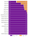 |
Fig. 1. Percentage of spaxels in each jellyfish galaxy that have a quenching probability PQ<0.3 (orange) and PQ>0.7 (purple). We consider a galaxy to be undergoing quenching when at least 4% of spaxels have PQ>0.7. |
We chose to only select galaxies as quenching jellyfish galaxies when at least 4% of the spaxels satisfied our quenching criterion. This removed A2744-09, where just a small fraction (0.7%) of the spaxels have PQ>0.7. The classification of a quenching jellyfish galaxy was assigned to six galaxies: A370-06, A370-08, A370-01, A370-03, A2744-06, and A2744-10. We focus on these galaxies when we present our results in the next section.
4. Properties of quenching jellyfish galaxies
4.1. Morphology of the quenched regions
Maps of PQ for our six quenching jellyfish are shown in Fig. 2. In five cases, we find quenched spaxels to be organized in arc-shaped regions at the leading edge of the galaxy disk (i.e., opposite to the tail). This configuration is observed in A2744-06, A2744-10, A370-01, A370-03, and A370-06. The pattern for A370-08 is more complex. Most of the quenched spaxels are found in the west (right side in the figure), but some signatures of quenching are also detected at the opposite end of the disk.
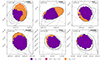 |
Fig. 2. Maps of the quenching probability PQ for the six jellyfish galaxies undergoing quenching. The probability is shown as a purple-to-orange color map. Orange indicates a high quenching probability. The solid black contours show the [O II]λ3727 flux maps, smoothed with a 3σ Gaussian kernel. The dashed black lines show the best-fit ellipse to the the shape of each galaxy (g-band flux 3σ above background); any spaxels within the ellipse that are not plotted did not satisfy our S/N criterion and were not assigned a classification. |
To quantify how quenched spaxels are distributed with respect to the tail, we defined the vectors vT and vQ: The tail vector vT connects the barycenter of the g-band luminosity of the galaxy (within the 3σ masks) to the center of the [O II]λ3727 line luminosity of the tail (outside the 3σ masks). The quenching vector vQ also has its origin at the 3σ g-band luminosity center, and its head is the PQ-weighted center of the galaxy (the average position of the spaxels weighted by PQ). We used these definitions to measure the quenching displacement

which is the magnitude of the projection of vQ in the direction of the tail. We plot dQ against ||vT|| for quenching jellyfish galaxies in Fig. 3, as well as the distribution of ||vT|| for other jellyfish galaxies. In the figure, both axes are normalized by the average radius Ra, which is the average of the major and minor axes of the best-fitting ellipse to the 3σ mask of the galaxy (dashed lines in Fig. 2).
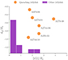 |
Fig. 3. Quenching displacement dQ against the length of the tail vector ||vT|| (see text for details) for quenching jellyfish galaxies (orange circles). The histogram of vT for other jellyfish galaxies is overplotted in purple. Both quantities are normalized by Ra. |
Positive values of dQ would indicate that quenched regions in the disk are found toward the direction of the tail, and negative values indicate that quenching mostly occurs at the opposite side, which is the case for all quenching jellyfish galaxies in our sample. The values of dQ serve to quantify the results that were noted through the visual inspection of Fig. 2, but they also (and more importantly) serve as a base framework that can be applied to larger samples in the future.
All quenching jellyfish galaxies have long tails (large ||vT||/Ra) when compared to what is measured for other jellyfish galaxies in our sample (see histogram in Fig. 3). As stated before in Sec. 3.4, a significant fraction of the disk spaxels of only 6 out of 18 jellyfish galaxies in our sample was classified as quenched. Fig. 3 shows, however, that when only galaxies with the longest tails are selected (||vT||>1.5 Ra), most of them (6 out of 8) undergo quenching.
4.2. Integrated spectra
We produced integrated spectra of regions with PQ>0.7 (quenched region) and PQ<0.3 in each of our quenching jellyfish galaxies, which we show in Fig. 4. These integrated spectra were used as part of the validation of our method, but they also carry important physical information.
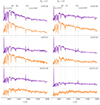 |
Fig. 4. Integrated spectra in the wavelength we used for our classification of the regions with PQ>0.7 (orange) and PQ<0.3 (purple) for our six quenching jellyfish galaxies. The spectra are plotted with arbitrary units. |
The galaxies in Fig. 4 are ordered as in Fig. 2, that is, in descending order of the fraction of quenched spaxels. The first three galaxies (A370-06, A370-08, and A370-01) show very strong Hδ and Hβ absorption lines in the integrated spectra of the quenched region, as is characteristic of the transition to a post-starburst phase. These features becomes less pronounced in galaxies with smaller quenched fractions, and they are barely noticeable in A2744-10, which is caught in an early phase of quenching. Moreover, the blue color (or triangular spectral shape) characteristic of post-starburst galaxies follows the same sequence. It is more prominent in the integrated spectra of the quenched regions in galaxies with higher quenched fractions.
Our ability to draw general conclusions from this small data set should not be overstated. The data presented in Fig. 4 indicate, however, that post-starburst features do not become strong until a relevant fraction of the stellar disk is stripped of gas. A hypothesis to explain this would be that star formation rates are enhanced toward the central regions of galaxies during stripping, which allows these regions to build up the stellar populations that give post-starburst spectra their characteristic shape, while gas in the outskirts is quickly stripped away before star formation can intensify. This idea is discussed further in Section 4.4.
4.3. Remaining ionized gas
Even in jellyfish galaxies undergoing quenching, a substantial fraction of spaxels (usually the majority) still show signatures of ionized gas. This gas is mainly concentrated in spaxels with low PQ, but it also appears in some of the quenched spaxels. In Fig. 5 we show BPT diagrams for our sample of quenching jellyfish to study their ionization sources. Only spaxels with relevant emission are plotted, that is, spaxels with S/N>3 in [O III]λ5007, Hβ, [N II]λ6584, and Hα. The emission line measurements are described in detail by Moretti et al. (2022).
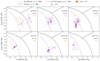 |
Fig. 5. BPT diagrams for spaxels in each of the six jellyfish galaxies undergoing quenching. Spaxels with PQ<0.3 are shown in purple, and spaxels with PQ>0.7 are shown in orange. The purple percentages show the fraction of spaxels with PQ<0.3 (not quenched) that satisfy the emission line S/N criteria for the diagram, and the orange percentages show the same for spaxels with PQ>0.7 (quenched). The lines in the diagrams show the classification boundaries from Kauffmann et al. (2003) (dotted line), Kewley et al. (2001) (dot-dashed line), and Cid Fernandes et al. (2011) (dashed line). |
Most galaxies in our sample have spaxels in the star-forming region of the BPT (below the Kauffmann et al. (2003) line) or in the so-called composite region (between the Kauffmann et al. 2003 and Kewley et al. 2001 lines). This composite emission may indicate a variety of processes and is frequently associated with diffuse ionized gas (see Lacerda et al. 2018).
The galaxy A370-06 stands out in the emission line classification because of the large portion of spaxels in the LINER region of the BPT. By inspecting the distribution of these spaxels in the galaxy, we see that they are spatially correlated with the tail and are not concentrated in the center of the stellar disk. We therefore conclude that this emission originates from extraplanar diffuse ionized gas in the tail and not from a LINER AGN.
As expected, most spaxels that were classified as quenched lack relevant emission lines and are therefore not included in the diagrams. The only galaxy in which a large fraction of quenched spaxels has emission lines is A370-06, which is reasonable as the ionization in this galaxies is caused by processes other than star formation. Our whole sample includes only one case of a spaxel with PQ>0.7 (classified as quenched) that has star-forming line ratios in the BPT (see the top right panel in Fig. 5 for A370-01). Fig. 2 also shows an island of spaxels with PQ<0.3 inside the arc of quenched spaxels in A370-01. This contrasts with the coeval quenched structures observed in other galaxies. The quenched spaxel with star-forming line ratios in A370-01 is found in the immediate vicinity of this island, which justifies this anomaly.
4.4. Star formation enhancement and the emergence of post-starburst features
Several works (e.g., Vulcani et al. 2018, 2020, 2024, but see also Boselli et al. 2023) showed that the star formation rates (SFR) in jellyfish galaxies are mildly enhanced when compared to typical star-forming galaxies, both globally and at kiloparsec scales. This enhancement can be associated with the compression of gas at the leading edge of the stellar disk (Bekki & Couch 2003; Roberts et al. 2022). At first glance, these results may seem at odds with the idea of ongoing quenching. There are at least two possibilities to reconcile these results: (i) The enhancement of the SFR may take place before the onset of quenching, in which case the quenching jellyfish should have a lower SFR than other jellyfish galaxies. (ii) On the other hand, the enhancement in the SFR in the star-forming spaxels of quenching jellyfish galaxies might be high enough to lead to a global enhancement even though star formation does not take place in the entire disk. To examine these possibilities, we compared the global and spatially resolved stellar mass – SFR relation or star-forming sequence (SFS) of quenching jellyfish galaxies with other jellyfish galaxies (see Fig. 6).
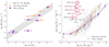 |
Fig. 6. Star formation rate vs. log stellar mass (log M★) for jellyfish galaxies in our sample. The left panel shows the integrated SFS with quenching jellyfish galaxies in orange and other jellyfish galaxies in purple. The best-fit line is shown as a dashed gray line, and the shaded region represents its uncertainty. The panel to the right shows the spatially resolved relation. The spaxels of all jellyfish galaxies are shown as gray background. The orange and purple lines trace the median trends for quenching and nonquenching jellyfish galaxies, respectively. The points are plotted in the center of each bin we used to trace the median trend, and the vertical lines trace the interquartile ranges. The inset in the right panel shows box plots of the difference |


The global SFRs (which only include BPT star-forming spaxels) and total stellar masses were taken directly from the tables of Vulcani et al. (2024). For the spatially resolved relation, stellar masses were obtained with SINOPSIS (Fritz et al. 2017), and the SFRs were calculated by applying the Kennicutt (1998) conversion to the Hα luminosity (adapted for a Chabrier 2003 IMF), corrected for dust extinction using a Cardelli et al. (1989) extinction curve with RV = 3.1, and assuming an intrinsic Balmer decrement Hα/Hβ = 2.86. The stellar mass and SFR of each spaxel were then divided by its area (in kpc2) to obtain the surface densities. The areas were deprojected using the axial ratio of the best-fit ellipse to the 3σ masks (see Sec. 2.2). This analysis was only performed when Hα fell in the observed spectral range and for spaxels in the galaxy disk (excluding tails) whose BPT line ratios were consistent with ionization by OB stars. Therefore, A370-06 and SMACS2031-01 were not included (see Fig. 5).
Somewhat unexpectedly, jellyfish galaxies undergoing quenching are typically at the high SFR end of the SFS of jellyfish galaxies. Out of the five quenching jellyfish galaxies included in Fig. 6, four are above the best-fit line, and only A370-08 (which has a very high quenched fraction; see Figures 1 and 2) is below this line. This indicates that the most significant SFR enhancement occurs during the quenching phase and that the global SFR only drops in the final stages of stripping (the case of A370-08), although low number statistics prevent us from generalizing this result. We also note that the SFS of jellyfish galaxies, which is the base of comparison in this analysis, is slightly above the one of normal star-forming galaxies (see Vulcani et al. 2024). This means that what we probe is an additional enhancement in comparison to an already enhanced relation.
This result is clarified by the spatially resolved SFS (right panel in Fig. 6). When compared to other jellyfish galaxies (purple line), the SFR surface density of quenching jellyfish galaxies (orange line) is enhanced in regions in which the stellar mass surface density is high. On the other hand, in regions in which the stellar mass surface density is low, the two groups follow a similar relation. We note that this result is biased by galaxy-to-galaxy variations. A2744-10 is enhanced throughout the entire disk, and all of its spaxels have  ; while A370-08 is in the opposite extreme. Its SFR is suppressed in all spaxels and
  . The remaining three galaxies (A2744-06, A370-01, and A370-03) follow almost identical relations that span the complete range of
  , and they are below the SFS of nonquenching jellyfish galaxies for
  and above it for
  .
.
Together, these results indicate a scenario in which the SFR is enhanced toward the central regions (high σM) in the earlier stages of stripping, but only after gas starts to be cleared out from the disk (see Fig. 3 and associated text). In the meantime, the gas in the outskirts of the disk is stripped away, leading to quenching, and eventually, the galaxy moves down in the SFS on its way to quiescence.
The idea of fast quenching in the outskirts coupled with a central SFR enhancement is in line with the stellar population gradients observed in cluster post-starburst galaxies (see Werle et al. 2022). The spatially resolved star formation histories of cluster post-starburst galaxies indicate that quenching must have occurred from the outside in, but also that star formation must have been boosted toward the center of the galaxy because the fraction of stellar mass that assembled a few hundred million years prior to quenching is higher in these regions. This comparison can be seen as additional evidence of ram pressure as the main driver of fast quenching in cluster environments, and it provides a direct assessment of how the properties of post-starburst galaxies (outside-in quenching with centrally concentrated bursts) in clusters are shaped under the effect of ram-pressure.
5. Conclusions
We have presented a systematic study of quenched regions in a sample of 18 jellyfish galaxies at intermediate redshift. Quenched regions were identified using a new method of spectral classification based on a one-dimensional CNN. This allowed us to characterize the frequency and spatial distribution of these regions, and we were able to compare jellyfish galaxies undergoing quenching to other jellyfish galaxies in order to understand their transition to quiescence. Our main results are listed below.
-
–
Signatures of ongoing quenching are detected in a significant fraction of the stellar disk in 6 out of 18 jellyfish galaxies. When we only considered the objects with the longest tails (||vT||>1.5Ra; see Fig. 3 and associated text), the detection rate of quenched regions is much higher (6 out of 8 galaxies).
-
–
Quenched regions are typically organized in arc-shaped regions and are concentrated at the leading edge of the disk (i.e., opposite to the tail; see Figures 2 and 3).
-
–
From the spatially resolved BPT classifications, we concluded that the galaxy with the highest quenched fraction (A370-06) lacks signs of star formation, and the only galaxy in which star formation is the only source of ionization in the disk is A2744-10, which is found to be in the very early stages of quenching.
-
–
The global SFRs of quenching jellyfish galaxies that still partially form stars are systematically higher than the SFR of other jellyfish galaxies, with the exception of A370-08, which is in an advanced stage of quenching. This occurs even though star formation does not take place in the entire disk.
-
–
The SFR enhancement in jellyfish galaxies undergoing quenching is concentrated in their central regions (high
 ; see Fig. 6), and the SFR can be as high as 0.5 dex above the SFS of other jellyfish galaxies. On the other hand, the SFR is typically suppressed in the outer regions, with the exception of A2744-10, which is in the very early stages of quenching and whose SFR is enhanced throughout its entire disk.
We presented early steps into a promising line of research. Our results indicate an evolutionary sequence in which star formation is enhanced when the disk starts to be cleared out of gas (Fig. 6) and post-starburst spectral features take shape as the stripping proceeds (Fig. 4). The relatively small sample size limits our ability to draw general conclusions, however. Furthermore, several issues such as the effect of wind direction, AGN activity, and infall velocity were left open. Exploring this science case in a large and diverse galaxy sample is key to broadening our view of the subject and to understanding to which extent our results are representative (Campbell et al. in prep).
Acknowledgments
We thank the anonymous referee for their critical appraisal of this paper. This project has received funding from the European Research Council (ERC) under the European Union's Horizon 2020 research and innovation program (grant agreement No. 833824, GASP project). B. V. and M. G. also acknowledge the Italian PRIN-Miur 2017 (PI A. Cimatti). We acknowledge funding from the INAF main-stream funding programme (PI B. Vulcani). J.F. acknowledges financial support from the UNAM- DGAPA-PAPIIT IN110723 grant, México.
When the age gradients between stellar populations in opposite sides of the stellar disk are strong (see Werle et al. 2022).
References
- Akerman, N., Tonnesen, S., Poggianti, B. M., Smith, R., & Marasco, A. 2023, ApJ, 948, 18 [NASA ADS] [CrossRef] [Google Scholar]
- Bekki, K., & Couch, W. J. 2003, ApJ, 596, L13 [NASA ADS] [CrossRef] [Google Scholar]
- Belli, S., Newman, A. B., & Ellis, R. S. 2019, ApJ, 874, 17 [Google Scholar]
- Boselli, A., Fossati, M., Roediger, J., et al. 2023, A&A, 669, A73 [NASA ADS] [CrossRef] [EDP Sciences] [Google Scholar]
- Bruzual, G., & Charlot, S. 2003, MNRAS, 344, 1000 [NASA ADS] [CrossRef] [Google Scholar]
- Campbell, S. 2024, PhD Thesis, University of St. Andrews, St. Andrews, UK [Google Scholar]
- Cardelli, J. A., Clayton, G. C., & Mathis, J. S. 1989, ApJ, 345, 245 [Google Scholar]
- Chabrier, G. 2003, PASP, 115, 763 [Google Scholar]
- Cid Fernandes, R., Stasińska, G., Mateus, A., & Vale Asari, N. 2011, MNRAS, 413, 1687 [Google Scholar]
- Cramer, W. J., Kenney, J. D. P., Cortes, J. R., et al. 2020, ApJ, 901, 95 [NASA ADS] [CrossRef] [Google Scholar]
- Croom, S. M., Lawrence, J. S., Bland-Hawthorn, J., et al. 2012, MNRAS, 421, 872 [NASA ADS] [Google Scholar]
- Ebeling, H., Edge, A. C., & Henry, J. P. 2001, ApJ, 553, 668 [Google Scholar]
- French, K. D. 2021, PASP, 133, 072001 [NASA ADS] [CrossRef] [Google Scholar]
- Fritz, J., Poggianti, B. M., Cava, A., et al. 2014, A&A, 566, A32 [NASA ADS] [CrossRef] [EDP Sciences] [Google Scholar]
- Fritz, J., Moretti, A., Gullieuszik, M., et al. 2017, ApJ, 848, 132 [NASA ADS] [CrossRef] [Google Scholar]
- George, K., Poggianti, B. M., Gullieuszik, M., et al. 2018, MNRAS, 479, 4126 [Google Scholar]
- George, K., Poggianti, B. M., Tomičić, N., et al. 2023, MNRAS, 519, 2426 [Google Scholar]
- Gullieuszik, M., Poggianti, B. M., Moretti, A., et al. 2017, ApJ, 846, 27 [Google Scholar]
- Gunn, J. E., Gott, J., & Richard, I. 1972, ApJ, 176, 1 [Google Scholar]
- Ignesti, A., Vulcani, B., Poggianti, B. M., et al. 2022a, ApJ, 937, 58 [NASA ADS] [CrossRef] [Google Scholar]
- Ignesti, A., Vulcani, B., Poggianti, B. M., et al. 2022b, ApJ, 924, 64 [NASA ADS] [CrossRef] [Google Scholar]
- Ignesti, A., Vulcani, B., Botteon, A., et al. 2023, A&A, 675, A118 [NASA ADS] [CrossRef] [EDP Sciences] [Google Scholar]
- Jáchym, P., Kenney, J. D. P., Sun, M., et al. 2019, ApJ, 883, 145 [Google Scholar]
- Kauffmann, G., Heckman, T. M., Tremonti, C., et al. 2003, MNRAS, 346, 1055 [Google Scholar]
- Kennicutt, R. C. Jr. 1998, ARA&A, 36, 189 [NASA ADS] [CrossRef] [Google Scholar]
- Kewley, L. J., Dopita, M. A., Sutherland, R. S., Heisler, C. A., & Trevena, J. 2001, ApJ, 556, 121 [Google Scholar]
- Lacerda, E. A. D., Cid Fernandes, R., Couto, G. S., et al. 2018, MNRAS, 474, 3727 [Google Scholar]
- Laudari, S., Jáchym, P., Sun, M., et al. 2022, MNRAS, 509, 3938 [Google Scholar]
- Loni, A., Serra, P., Sarzi, M., et al. 2023, MNRAS, 523, 1140 [CrossRef] [Google Scholar]
- Lotz, J. M., Koekemoer, A., Coe, D., et al. 2017, ApJ, 837, 97 [Google Scholar]
- Moretti, A., Paladino, R., Poggianti, B. M., et al. 2020, ApJ, 889, 9 [Google Scholar]
- Moretti, A., Radovich, M., Poggianti, B. M., et al. 2022, ApJ, 925, 4 [NASA ADS] [CrossRef] [Google Scholar]
- Owers, M. S., Hudson, M. J., Oman, K. A., et al. 2019, ApJ, 873, 52 [Google Scholar]
- Paccagnella, A., Vulcani, B., Poggianti, B. M., et al. 2017, ApJ, 838, 148 [NASA ADS] [CrossRef] [Google Scholar]
- Paccagnella, A., Vulcani, B., Poggianti, B. M., et al. 2019, MNRAS, 482, 881 [NASA ADS] [CrossRef] [Google Scholar]
- Pawlik, M. M., Taj Aldeen, L., Wild, V., et al. 2018, MNRAS, 477, 1708 [Google Scholar]
- Peng, Y., Maiolino, R., & Cochrane, R. 2015, Nature, 521, 192 [Google Scholar]
- Poggianti, B. M., Smail, I., Dressler, A., et al. 1999, ApJ, 518, 576 [Google Scholar]
- Poggianti, B. M., Bridges, T. J., Komiyama, Y., et al. 2004, ApJ, 601, 197 [NASA ADS] [CrossRef] [Google Scholar]
- Poggianti, B. M., Aragón-Salamanca, A., Zaritsky, D., et al. 2009, ApJ, 693, 112 [NASA ADS] [CrossRef] [Google Scholar]
- Poggianti, B. M., Fasano, G., Omizzolo, A., et al. 2016, AJ, 151, 78 [Google Scholar]
- Poggianti, B. M., Moretti, A., Gullieuszik, M., et al. 2017, ApJ, 844, 48 [Google Scholar]
- Poggianti, B. M., Ignesti, A., Gitti, M., et al. 2019, ApJ, 887, 155 [Google Scholar]
- Postman, M., Coe, D., Benítez, N., et al. 2012, ApJS, 199, 25 [Google Scholar]
- Richard, J., Claeyssens, A., Lagattuta, D., et al. 2021, A&A, 646, A83 [EDP Sciences] [Google Scholar]
- Roberts, I. D., van Weeren, R. J., McGee, S. L., et al. 2021, A&A, 650, A111 [NASA ADS] [CrossRef] [EDP Sciences] [Google Scholar]
- Roberts, I. D., Lang, M., Trotsenko, D., et al. 2022, ApJ, 941, 77 [NASA ADS] [CrossRef] [Google Scholar]
- Rohr, E., Pillepich, A., Nelson, D., et al. 2023, MNRAS, 524, 3502 [NASA ADS] [CrossRef] [Google Scholar]
- Schawinski, K., Urry, C. M., Simmons, B. D., et al. 2014, MNRAS, 440, 889 [Google Scholar]
- Serra, P., Maccagni, F. M., Kleiner, D., et al. 2023, A&A, 673, A146 [NASA ADS] [CrossRef] [EDP Sciences] [Google Scholar]
- Stuik, R., Bacon, R., Conzelmann, R., et al. 2006, New Astron. Rev., 49, 618 [CrossRef] [Google Scholar]
- Sun, M., Ge, C., Luo, R., et al. 2021, Nat. Astron., 6, 270 [NASA ADS] [CrossRef] [Google Scholar]
- Treu, T., Schmidt, K. B., Brammer, G. B., et al. 2015, ApJ, 812, 114 [Google Scholar]
- Vulcani, B., Poggianti, B. M., Jaffé, Y. L., et al. 2018, MNRAS, 480, 3152 [NASA ADS] [CrossRef] [Google Scholar]
- Vulcani, B., Fritz, J., Poggianti, B. M., et al. 2020, ApJ, 892, 146 [Google Scholar]
- Vulcani, B., Poggianti, B. M., Smith, R., et al. 2022, ApJ, 927, 91 [NASA ADS] [CrossRef] [Google Scholar]
- Vulcani, B., Moretti, A., Poggianti, B. M., et al. 2024, A&A, 682, A117 [NASA ADS] [CrossRef] [EDP Sciences] [Google Scholar]
- Werle, A., Cid Fernandes, R., Vale Asari, N., et al. 2019, MNRAS, 483, 2382 [Google Scholar]
- Werle, A., Poggianti, B., Moretti, A., et al. 2022, ApJ, 930, 43 [NASA ADS] [CrossRef] [Google Scholar]
- Wild, V., Almaini, O., Dunlop, J., et al. 2016, MNRAS, 463, 832 [NASA ADS] [CrossRef] [Google Scholar]
- Wilkinson, S., Ellison, S. L., Bottrell, C., et al. 2022, MNRAS, 516, 4354 [CrossRef] [Google Scholar]
- York, D. G., Adelman, J., Anderson, J. E. Jr., et al. 2000, AJ, 120, 1579 [Google Scholar]
All Tables
All Figures
|
Fig. 1. Percentage of spaxels in each jellyfish galaxy that have a quenching probability PQ<0.3 (orange) and PQ>0.7 (purple). We consider a galaxy to be undergoing quenching when at least 4% of spaxels have PQ>0.7. |
| In the text | |
|
Fig. 2. Maps of the quenching probability PQ for the six jellyfish galaxies undergoing quenching. The probability is shown as a purple-to-orange color map. Orange indicates a high quenching probability. The solid black contours show the [O II]λ3727 flux maps, smoothed with a 3σ Gaussian kernel. The dashed black lines show the best-fit ellipse to the the shape of each galaxy (g-band flux 3σ above background); any spaxels within the ellipse that are not plotted did not satisfy our S/N criterion and were not assigned a classification. |
| In the text | |
|
Fig. 3. Quenching displacement dQ against the length of the tail vector ||vT|| (see text for details) for quenching jellyfish galaxies (orange circles). The histogram of vT for other jellyfish galaxies is overplotted in purple. Both quantities are normalized by Ra. |
| In the text | |
|
Fig. 4. Integrated spectra in the wavelength we used for our classification of the regions with PQ>0.7 (orange) and PQ<0.3 (purple) for our six quenching jellyfish galaxies. The spectra are plotted with arbitrary units. |
| In the text | |
|
Fig. 5. BPT diagrams for spaxels in each of the six jellyfish galaxies undergoing quenching. Spaxels with PQ<0.3 are shown in purple, and spaxels with PQ>0.7 are shown in orange. The purple percentages show the fraction of spaxels with PQ<0.3 (not quenched) that satisfy the emission line S/N criteria for the diagram, and the orange percentages show the same for spaxels with PQ>0.7 (quenched). The lines in the diagrams show the classification boundaries from Kauffmann et al. (2003) (dotted line), Kewley et al. (2001) (dot-dashed line), and Cid Fernandes et al. (2011) (dashed line). |
| In the text | |
|
Fig. 6. Star formation rate vs. log stellar mass (log M★) for jellyfish galaxies in our sample. The left panel shows the integrated SFS with quenching jellyfish galaxies in orange and other jellyfish galaxies in purple. The best-fit line is shown as a dashed gray line, and the shaded region represents its uncertainty. The panel to the right shows the spatially resolved relation. The spaxels of all jellyfish galaxies are shown as gray background. The orange and purple lines trace the median trends for quenching and nonquenching jellyfish galaxies, respectively. The points are plotted in the center of each bin we used to trace the median trend, and the vertical lines trace the interquartile ranges. The inset in the right panel shows box plots of the difference |
| In the text | |
Current usage metrics show cumulative count of Article Views (full-text article views including HTML views, PDF and ePub downloads, according to the available data) and Abstracts Views on Vision4Press platform.
Data correspond to usage on the plateform after 2015. The current usage metrics is available 48-96 hours after online publication and is updated daily on week days.
Initial download of the metrics may take a while.