| Issue |
A&A
Volume 699, July 2025
|
|
|---|---|---|
| Article Number | A36 | |
| Number of page(s) | 17 | |
| Section | Numerical methods and codes | |
| DOI | https://doi.org/10.1051/0004-6361/202453293 | |
| Published online | 27 June 2025 | |
The AI supervisor of source-extraction algorithms for images obtained by wide-field small-aperture optical telescopes
1
College of Physics and Optical Engineering, Taiyuan University of Technology, Taiyuan,
Shanxi,
030024,
China
2
National Astronomical Observatories,
Beijing
100101,
China
★ Corresponding author: This email address is being protected from spambots. You need JavaScript enabled to view it.
Received:
4
December
2024
Accepted:
7
May
2025
Abstract
Aims. Wide-field small-aperture optical telescopes are essential for the imaging of celestial objects for time-domain astronomy. The extraction positions and magnitudes of celestial objects within observation images are a key prerequisite for carrying out further scientific results. The parameters of the source-extraction algorithms must be fine-tuned to achieve an optimal performance. This can be time-consuming and resource intensive.
Methods. Inspired by the manual parameter fine-tuning procedure, we propose the concept of an AI supervisor for source-extraction algorithms based on reinforcement learning. Firstly, we built an AI supervisor with deep neural networks and generated simulated images based on configurations of the observation instruments and various observation conditions as prior information. Then, we trained the AI supervisor with simulated and real observation images, with the ground-truth catalogue and magnitudes of reference stars as the desired output. Upon completion of training, the AI supervisor can obtain the optimal parameters of the source-extraction algorithms for newly acquired images through automatically fine-tuning based on prior information about the observation conditions and on the properties of the observed star fields.
Results. We evaluated the AI supervisor using simulated and real observation images. The results indicate that the AI supervisor effectively identifies the optimal parameters for the source-extraction algorithm in processing newly observed images within a few iterations. With these optimised parameters, the source-extraction algorithm achieves a higher photometry accuracy, higher precision rates, and a lower detection threshold. These enhancements underline the potential of the AI supervisor in fine-tuning source-extraction algorithms and other related astronomical data-processing algorithms.
Key words: methods: data analysis / techniques: image processing / telescopes
© The Authors 2025
 Open Access article, published by EDP Sciences, under the terms of the Creative Commons Attribution License (https://creativecommons.org/licenses/by/4.0), which permits unrestricted use, distribution, and reproduction in any medium, provided the original work is properly cited.
This article is published in open access under the Subscribe to Open model. This email address is being protected from spambots. You need JavaScript enabled to view it. to support open access publication.
1 Introduction
As the construction of telescopes for astronomical observations continues to grow, astronomers are able to acquire an extensive volume of observation images (Kaiser 2004; Rau et al. 2009; Udalski et al. 2015; Tonry et al. 2018; Ivezić et al. 2019; Bellm et al. 2019; Kou 2019; Lokhorst et al. 2020; Xu et al. 2020; Dyer et al. 2020; Liu et al. 2021; Law et al. 2022; Beskin et al. 2023). These images, taken at various observational bands and in different time periods, reveal the activities of celestial objects and enable scientists to uncover numerous intriguing phenomena. These include time-domain astronomical events, which show the transient activities of celestial objects over short periods, and are especially captivating. Examples of these time-domain astronomical events include exoplanets, stellar flares, tidal disruption events, supernovae, and optical counterparts of gravitational-wave events (Castro-Tirado et al. 1999; Gal-Yam et al. 2006, 2011; Gromadzki et al. 2019; Han et al. 2021; Steeghs et al. 2022; Jia et al. 2023c). Studying these events requires the fast processing of astronomical images because follow-up observations are essential for capturing signals from different regions of these celestial objects shortly after the time-domain events occur.
In the astronomical image-processing pipeline, source extraction algorithms play a pivotal role. They automatically detect celestial objects and carry out photometry of these celestial objects. The ongoing evolution of these algorithms has given rise to various source-extraction codes that range from traditional methods such as SExtractor (Bertin & Arnouts 1996), imagexy (Lang et al. 2010), and mathematical morphology methods (Sun et al. 2022) to novel approaches based on deep neural networks (Cabrera-Vives et al. 2017; Andreon et al. 2000; Jia et al. 2020; Panes et al. 2021; He et al. 2021; Casas et al. 2022; Rezaei et al. 2022; Stoppa et al. 2023). These advancements have progressively enhanced the speed, photometry precision, detection precision, and detection limits of the source-extraction algorithms. Source-extraction algorithms incorporate numerous parameters that significantly influence the quality of the final results, however, including the detection thresholds, the minimally connected regions, the photometry aperture, the learning rates, and the training set composition. The parameters of the source-extraction algorithms represent a critical consideration in the astronomical data-processing. The multitude of configurable parameters necessitates careful optimisation, as each parameter selection directly affects the detection precision, the detection limits, and the reliability of the photometry results. While manually obtained parameter settings by scientists are generally thought to yield acceptable detection outcomes, numerous iterations are required to achieve this, and they demand considerable time and human effort (Axelrod et al. 2004; Masci et al. 2018; Myers et al. 2023). The challenge is further compounded in time-domain astronomy observations, where the sky background level, seeing conditions, telescope status, and properties of the star fields change dynamically. This variability makes it a challenge to manually select the best parameters for each image in a time-efficient manner. Consequently, there is a pressing need for novel methods to fine-tune the parameters of the source-extraction algorithms to ensure an optimal performance in varying observational conditions.
Various methods are currently used to determine the optimal parameters in source-extraction algorithms. The traditional approach involves a manual parameter-tuning based on empirical knowledge, under the assumption that images captured by the same telescope on adjacent observation dates possess similar properties. In this method, scientists initially fine-tune the parameters using several example images and verify the source-extraction results manually. Although effective, this process requires substantial expertise and involves significant trial and error to achieve satisfactory outcomes. Sky survey telescopes that are commonly used for time-domain astronomy observations typically feature relatively small apertures and wide fields of view, which leads to lower limiting magnitudes. Consequently, researchers can refer to the magnitudes of reference stars and catalogues obtained from telescopes with higher limiting magnitudes, and they can employ grid-search methods to determine the optimal parameters for the source-extraction algorithms for each image. Additionally, heuristic algorithms, such as genetic algorithms (Mirjalili & Mirjalili 2019), can be applied to expedite the search process. These methods demand substantial computational resources and time to identify the optimal parameters for each image, however. When the observational conditions vary, the performance often deteriorates, which necessitates further optimisation searches.
Upon further examination of the philosophy in the fine-tuning parameters of source-extraction algorithms, another potential solution emerges. Inspired by bionics, we can treat the application of source-extraction algorithms to processing astronomical images as an interactive and iterative process. Initially, scientists set the algorithm parameters based on prior visual information extracted from astronomical images, considering key factors such as sky background levels, the full width at half maximum (FWHM) of the point spread function (PSF), the magnitudes of reference stars, and the number of stars with various magnitudes throughout the entire magnitude range above the detection limit. Following this initial setup, scientists review the detection results and photometry results, and they then adjust the parameters based on their prior knowledge. For example, when the algorithm detects fewer low-magnitude stars than expected, scientists may lower the detection threshold. Conversely, they may raise the threshold when too many false positives are detected. By following these steps, suitable parameters for source-extraction algorithms can be obtained to process observed images.
Since AI is fundamentally designed to emulate human intelligence (Turing 2004; Poole & Mackworth 2010), we developed an AI supervisor to automatically fine-tune the parameters of source-extraction algorithms in this paper. The AI supervisor operates within a reinforcement learning framework, mimicking the manually parameter fine-tuning process for images acquired with a particular telescope (Arulkumaran et al. 2017). Taking the parameters in the source detection algorithm as an example: we first of all trained the neural network to obtain the parameters in source detection algorithms according to current detection results and qualities of observation images. To do this, we used simulated images that represent a variety of observation conditions, and we employed the digital twin concept to import essential knowledge to the system (Zhan et al. 2022; Jia et al. 2022; Zhang et al. 2023; Jia et al. 2023a). We also used the reward function to include the prior information of the images that were to be processed. During the training step, the ground-truth catalogue was used to evaluate the performance of the source-detection algorithm. During the deployment stage, the density and distribution of stars at different magnitudes was used as performance evaluation criteria. The AI supervisor uses all detected targets to determine the distribution of stars at different magnitudes. This enables us to compare the predictions from the catalogue and the detection results, and we can further refine the source-detection algorithm parameters accordingly. Through several iterations, the framework achieves optimal parameters for the source detection algorithms for a specific image.
This paper is organised as follows. In Sect. 2, we introduce the concept of our method. Sect. 3 details the application scenario and discusses our strategy for generating simulated data. Sect. 4 discusses application details of our method in processing time-domain astronomical images. Finally, Sect. 5 summarises the paper and proposes directions for future research.
2 Design of the Al supervisor for the source-extraction algorithms
2.1 Philosophy of the AI supervisor
Since the pioneering work on ImageNet (Deng et al. 2009), the domain of computer vision has undergone significant advancements. The exceptional performance of AlexNet (Alom et al. 2018) in the ImageNet Large Scale Visual Recognition Challenge (ILSVRC) has catalysed the creation of various deep neural networks (Russakovsky et al. 2015), such as Fast R-CNN (Girshick 2015), Faster R-CNN (Ren et al. 2015), Mask RCNN (He et al. 2017), YOLO (Jiang et al. 2022), and Vision Transformer models (Han et al. 2022). By leveraging large training datasets and employing effective training methods, these advanced deep neural networks can be proficiently trained and used across a broad array of computer vision tasks. These applications include image classification, object detection, and image segmentation, which highlights the versatility and efficacy of contemporary deep-learning techniques in the realm of visual perception and analysis.
The extraction of astronomical targets in images resembles the object-detection techniques discussed in the computer vision area. Both methods focus on locating objects, categorising them into established classifications, and obtaining their properties. In the context of astronomy, these objects include celestial entities such as stars, planets, and galaxies. Due to this similarity, various algorithms that were originally developed for computer vision have been adapted for use in astronomical image processing (Cabrera-Vives et al. 2017; Andreon et al. 2000; Jia et al. 2020; Panes et al. 2021; He et al. 2021; Casas et al. 2022; Rezaei et al. 2022; Stoppa et al. 2023). The fundamental principle is simple: By using a dataset that reflects the qualities of astronomical images and our specific requirements, we can train a neural network to analyse real observational images. The algorithms from the computer vision field are generally tailored for processing ordinary images, however. As a result, they often focus on a limited range of grey levels (typically, 28 levels), consist of three colour channels (red, green, and blue), and accommodate only a small number of objects in one image (ranging from one to a few dozen). To address the specific needs of astronomical research, new algorithms have been developed. These advancements include models capable of processing images with varying numbers of channels (Jia et al. 2023b) and algorithms that offer uncertainty estimates regarding the positions and magnitudes of celestial objects (Sun et al. 2023). These developments are essential for a precise and reliable data analysis in the field of astronomy.
Despite the advancement of various source-extraction algorithms, a persistent challenge remains: fine-tuning of parameters within source-extraction algorithms. This issue is important in deep learning based source-extraction algorithms, where the composition of training data and the selection of detection thresholds (or confidence levels) significantly influence algorithm performance. For instance, employing a higher confidence threshold generally yields detection results with higher precision but lower recall rates, leading to more accurate detections while potentially overlooking fainter stars. The challenge also arises in traditional source-extraction algorithms such as the SExtractor. Parameters that are typically adjusted in SExtractor include the detection threshold and the minimal connected region for the detection part and the aperture size for the photometry part. The extensive range of free parameters across different source-extraction algorithms poses a substantial difficulty in selecting appropriate parameters for different algorithms to process real observational data, a dilemma referred to as the parameter optimisation problem (Rix et al. 2004) (termed the parameter fine-tuning problem in this paper). While foundational research has tackled this issue for traditional target-detection algorithms and proposed strategies for parameter fine-tuning (Haigh et al. 2021), there remains a lack of in-depth studies that could facilitate the automatic tuning of parameters for images with varying qualities.
Deep neural network based source-extraction algorithms, which belongs to supervised learning, have gained significant traction in the astronomy community as a form of AI. Another AI method known as reinforcement learning (RL) has not been as widely discussed in astronomical research. However, unlike supervised learning, which depends on predefined correct answers, or unsupervised learning, which identifies inherent relationships within data, RL focuses on an agent that learns through trial and error, using feedback from its actions. A landmark achievement in RL occurred in 2016 when Google DeepMind’s AlphaGo triumphed over Go champion Lee Sedol with a score of 4:1 (Silver et al. 2016). When an agent is constructed using deep neural networks, this method is referred to as deep reinforcement learning (DRL). Subsequent advancements, such as AlphaGo Master and AlphaGo Zero, further illustrated the potential of DRL. DRL provides considerable advantages in navigating complex environments and enhancing generalisation. It is capable of training in environments that are difficult to articulate and can use deep neural networks to generalise to previously unseen states, thereby presenting significant opportunities for practical applications (Yatawatta 2024). The astronomy community has recently begun investigating the applications of DRL, including its use in managing adaptive optics systems (Nousiainen et al. 2022), optical telescopes (Jia et al. 2023c), and radio telescopes (Yatawatta & Avruch 2021). A recent study has indicated that DRL could aid astronomers in addressing radio data calibration and processing tasks (Yatawatta 2023), which represent some of the most intricate data processing challenges within the field.
The parameter fine-tuning procedure for source-extraction algorithms used in processing images obtained by wide-field small-aperture optical telescopes can be effectively conceptualised within the framework of DRL. Within the DRL framework, fine-tuning of parameters for source-extraction algorithms can be viewed as the action, while the current configuration of these parameters represents the state. For photometry tasks, reward functions can be formulated to minimise photometric error between measured and expected values. Meanwhile, when addressing detection tasks, reward functions can be constructed to quantify the disparity in stellar density distributions across magnitude ranges, comparing the processed output against reference catalogues. By delineating the state, the action, and the reward within an optimisation algorithm, we empower the AI supervisor to fine-tune the source-extraction parameters according to the prevailing conditions. This method promotes the automatic adjustment of source-extraction algorithm parameters to accommodate varying observational environments and target characteristics. The subsequent sections will delve into the comprehensive design of this DRL implementation (the AI supervisor in this paper), illustrating how this innovative approach can improve the efficiency of source-extraction algorithms.
2.2 State, action, and reward of the AI supervisor
Drawing from the principles previously outlined, this section will illustrate the construction of an AI supervisor designed to fine-tune the parameters of source-extraction algorithms. The AI supervisor receives the observation image as input and produces optimised parameters for the source-extraction algorithm as output. Specifically, we will focus on processing images obtained by wide field small aperture telescopes with photometry and target detection within the SExtractor. These telescopes, which are generally used for sky surveys in time-domain astronomy, are characterised by apertures of less than 1 meter and fields of view that extend to several degrees or more (Jia et al. 2017; Bialek et al. 2024). In real observations, these telescopes continuously acquire short-exposure images, which are often affected by various factors, such as variations in PSF and fluctuating sky backgrounds. Given the urgency of processing these images swiftly to facilitate subsequent observations, there is a pressing need to design an AI supervisor that can automatically determine the optimal parameters, thereby accelerating the follow-up observation process.
SExtractor is selected for this purpose due to its proven capability in processing a broad range of observational images, establishing it as a well-regarded tool within the field (Bertin & Arnouts 1996). The performance of SExtractor, however, hinges on the meticulous adjustment of numerous parameters that influence both object detection and subsequent photometric accuracy. This study concentrates on two key detection parameters: the detection threshold and the minimum number of connected pixels exceeding this threshold required for a detection. These parameters are critical in defining the precision and sensitivity of the detection process. For photometry, SExtractor offers both fixed-aperture and automatic-aperture methods. In this work, we leverage reinforcement learning to optimise the aperture size for fixed-aperture photometry. Given the complexity of SExtractor, which encompasses functionalities beyond photometry and detection algorithms, we use a streamlined, GPU-based implementation of detection and photometry defined in the SExtractor in this study (Cao et al. 2025). The concepts of states, actions, and rewards are essential components of DRL. We treat detection and photometry as separate tasks, recognising that each possesses distinct parameter optimisation objectives and, consequently, necessitated individual optimisation strategies. Therefore, we detail the state space, action space, and reward function independently for each task in the subsequent subsections. Finally, we describe how these individual algorithms can be integrated to form a comprehensive framework.
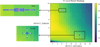 |
Fig. 1 Two-dimensional heat map representing the parameter distribution of the detection threshold (DETECT_THRESH) and the minimally connected regions (DETECT_MINAREA) for the target-detection task in a specific image, thus providing a visual depiction of the state distribution. The depiction of the designed states and actions is presented in the left panel. The current parameter position is denoted as (i, j), and the four adjacent positions are identified as (i+1, j), (i-1, j), (i, j+0.1), and (i, j-0.1). |
2.2.1 State, action, and reward of the AI supervisor for the source-detection part
The state reflects the current environment as interpreted by the AI supervisor, embodying its comprehension of both the surrounding context and the specific task. For the task of parameter fine-tuning in source detection part, we used different state representation methods during the training and deployment phases. During the training phase, where the catalogue was known, the state was defined as the F1-score of the target-detection algorithm using the current parameter sets, together with the F1-scores of its four adjacent states (up, down, left, right). There were four adjacent states, because we needed to fine-tune 2 separate parameters. The detection algorithm calculates the F1-score for the current state, subsequently evaluating the F1-scores for each of the four adjacent states. These five F1-scores were then combined to form the overall state, which was subsequently input into the network to determine the appropriate action to be taken.
In the deployment phase, while the specific details of the catalog remained unknown, information regarding the number of stars of varying magnitudes can be inferred based on the field of view, pointing direction, and limiting magnitude. As a result, we substituted the F1-score with a combination of the Kullback-Leibler (KL) divergence, representing the slope of the star distribution, and the total number of stars that were above the detection limit, to define the state. The top left panel in Fig. 1 shows the distribution of states in the detection task for an image.
The action space comprises the set of actions that the AI supervisor selects based on its current state. An effectively structured action space enhances the AI supervisor’s perception and interaction with the environment. In the source detection part, actions are defined as the adjustments of parameters (minimal connected regions and detection threshold), as shown in Fig. 1. We established various step sizes for these two parameters, with their selection guided by the AI supervisor during the exploration process. The action space was defined by the ranges and increments of each parameter. For minimal connected regions, the range extended from 1 to 20 pixels, with step changes ranging from −5 to 5 pixels at intervals of 1 pixel, yielding 10 possible values. The range for detection threshold spanned from 0.5 to 10, with step changes ranging from −1 to 1 at intervals of 0.1, resulting in 21 possible values. Thus, the action space encompassed 210 unique combinations.
The reward is a scalar provided by the environment, reflecting the performance of the AI supervisor’s strategy at a specific step. The objective of the AI supervisor is to maximise the reward. In this context, the AI supervisor strived to maximise its expected cumulative reward. During the training phase, we aimed to enable the AI supervisor to identify optimal parameters that detect the maximum number of stars above the detection limit and keep the false-detection rates of the results low. For this purpose, we used the catalogue as a reference and calculate the F1-Score, as described in Eq. (1), to estimate the reward,
![Mathematical equation: $\[\begin{aligned}\text {Precision} & =\frac{T P}{T P+F P}, \\\text {Recall} & =\frac{T P}{T P+F N}, \\\text {F1-Score} & =\frac{{Recall} \times {Precision}}{{Recall}+ { Precision }},\end{aligned}\]$](/articles/aa/full_html/2025/07/aa53293-24/aa53293-24-eq1.png) (1)
(1)
where T P denotes the number of detection results classified as true celestial objects, F P represents the number of detection results categorised as false positives (non-celestial objects), and F N stands for number of stars that are not detected by the algorithm. According to the ground truth catalogue, the F1-score is integrated with Eq. (2) as the reward:
![Mathematical equation: $\[\begin{aligned}\Delta F 1_n & =F 1_n-F 1_{n-1} \quad(\text { Adjacent F1-score difference }) \\\Delta F 1_{max } & =F 1_0-F 1_n \quad(\text { Ground-truth F1-score difference }) \\\text { Reward } & =\left\{\begin{array}{l}100 \cdot \Delta F 1, \\\text { if }\left(\Delta F 1_{max }>a\right) \wedge\left(\Delta F 1_n>0.2 \vee \Delta F 1_n<-0.1\right) \\400 \cdot \Delta F 1, \\\text { if }\left(\Delta F 1_{max } \leq a\right) \wedge\left(\Delta F 1_n>0.05 \vee \Delta F 1_n<0\right) \\-2, \\\text { otherwise, }\end{array}\right.\end{aligned}\]$](/articles/aa/full_html/2025/07/aa53293-24/aa53293-24-eq2.png) (2)
(2)
where F10 is the detection limit of the detection algorithm with optimal parameter set, which is obtained through grid search method. F1n and F1n–1 are F1-score of the contemporary state and adjacent state, ΔF1n is difference of F1-score between contemporary state and adjacent states, ΔF1max is difference of F1-score between contemporary state and the optimal state. a is a parameter to make trade-off between contemporary F1-score and optimal F1-score.
During the deployment phase, the AI supervisor lacks specific information regarding positions and magnitudes of celestial objects. According to the sky background, however, the FWHM of the PSF, the diameter of the telescope, and the pixel scale of the observational image, we could determine the limiting magnitude. Additionally, since we knew the field of view, the pixel scale of the telescope, and a catalogue with a lower detection limit, we could approximate the total number of stars present in the observational images, as well as produce a histogram of stars with different magnitudes. While the final detection results may differ from those provided by the catalogue – due to transient events or variable star magnitudes – these deviations were expected to be minimal. Consequently, we employed the following equation as the basis for the reward as shown in Eq. (4),
![Mathematical equation: $\[\begin{aligned}\mathrm{KL} & =D_{K L}(P \| Q)=\sum_{mag} P({ mag }) \log \left(\frac{P({ mag })}{Q({ mag })}\right), \\\text { Numdiff } & =\frac{({ DetNum }- { GroundNum })^2}{{ GroundNum }},\end{aligned}\]$](/articles/aa/full_html/2025/07/aa53293-24/aa53293-24-eq3.png) (3)
(3)
where P(mag) and Q(mag) represent the magnitude distributions of stars from the catalogue and from our photometry results, respectively. Although we aimed to determine the optimal aperture size based on the magnitudes of reference stars in the photometry part, a slight risk remains that the photometry may be uncalibrated. To mitigate this, we aligned the zero points of P(mag) and Q(mag). Additionally, DetNum and GroundNum stand for number of stars obtained by the detection algorithm and the ground truth number of stars that are above the detection limit within the field of view. KL represents the difference between the distribution of the detected stars and stars in the catalogue, where a smaller KL indicates that the detection results are more similar to the catalogue, and the model’s prediction accuracy is higher. Meanwhile, Numdiff signifies the difference between stars listed in the catalogue that exceed the detection limit and those identified by the algorithm. The smaller the value of Numdiff, the closer the model’s detection results are to the true situation, and the smaller the error. With these two metrics, we are able to evaluate the performance of the model.
During the deployment phase, the goal is to minimise the difference between KL and Numdiff, which indicates that the results obtained by the detection algorithm are closer to the catalogue, as shown in Eq. (4),
![Mathematical equation: $\[\begin{aligned}w_{\mathrm{KL}} & =\frac{\mathrm{KL}}{\mathrm{KL}+\text { Numdiff }} \\w_{\text {Numdiff }} & =\frac{\text { Numdiff }}{\mathrm{KL}+\text { Numdiff }} \\\text { Reward } & =\left\{\begin{array}{r}-w_{\mathrm{KL}} \cdot \Delta \mathrm{KL}-w_{\text {Numdiff }} \cdot \Delta \text { Numdiff } \\\text { if } \Delta \mathrm{KL}>0 \text { or } \Delta \mathrm{Numdiff}>0 \\w_{\mathrm{KL}} \cdot|\Delta \mathrm{KL}|+w_{\text {Numdiff }} \cdot|\Delta \mathrm{Numdiff}| \\\text { if } \Delta \mathrm{KL} \leq 0 \text { and } \Delta \text { Numdiff } \leq 0\end{array}\right.\end{aligned}\]$](/articles/aa/full_html/2025/07/aa53293-24/aa53293-24-eq4.png) (4)
(4)
where wKL and wNumdiff are weights obtained from KL and Numdiff. According to the definition above, we could find that when the KL is larger, which means that the difference of the detection results between stars of different magnitudes is more pronounced, the AI supervisor modified the parameters to obtain reasonable results; when the Numdiff is larger, which means that there are significant differences between stars with different numbers, the AI supervisor modified the parameters accordingly. Through this design, the changes in KL and Numdiff dynamically adjusted their weights according to their impact on the overall error. This ensures that the reward reflects the model performance reasonably well in different error scenarios.
2.2.2 State, action, and reward of the AI supervisor for the photometry part
For the photometry task, we implemented the AI supervisor to optimise aperture sizes in fixed-aperture photometry. Our state representation incorporated photometric errors from both the current aperture configuration and adjacent parameter settings, creating a comprehensive error landscape representation. The AI supervisor constructed the state vector by first calculating photometric error using base aperture parameters as the foundational component. It then computed errors for adjacent aperture configurations using predefined offsets, assembling these values into a composite state representation. This multidimensional vector underwent flattening into a one-dimensional array to satisfy the input requirements of deep reinforcement learning algorithms. Through this approach, the AI supervisor developed awareness of both current performance and the surrounding error gradient, enabling more informed parameter adjustments. The action space for photometry task discussed in this paper encompassed aperture size variations ranging from 0.5 to 20.0 pixels, with adjustment steps of ±0.5 pixel and a fine-grained incremental interval of 0.02 pixel. This configuration yielded 51 distinct parameter combinations, allowing the AI supervisor to explore the parameter space with sufficient granularity to optimise the photometric accuracy. The mathematically defined range can be expressed as (A = ai|ai ∈ [0.5, 20.0], ai+1 − ai = 0.02), where A represents the complete set of possible aperture configurations.
The reward function directs parameter optimisation by quantifying the differential between the updated photometric error errn and its predecessor err. The AI supervisor received a positive reward when errn < err, indicating improved performance, and conversely incurred a negative penalty when performance deteriorates. Critically, the magnitude of this reward or penalty scaled proportionally with the absolute difference between error values, creating a gradient that reflected the significance of each parameter adjustment. This proportional scaling ensures that substantial improvements yield correspondingly substantial rewards, while minor degradations result in appropriate penalties. The definition of the reward function is shown in Equation (5):
![Mathematical equation: $\[R= \begin{cases}1+\left(e r r-e r r_n\right) \cdot 30, & \text { if } e r r_n<e r r, \\ -1-\left(e r r_n-e r r\right) \cdot 20, & \text { if } e r r_n \geq e r r.\end{cases}\]$](/articles/aa/full_html/2025/07/aa53293-24/aa53293-24-eq5.png) (5)
(5)
The reward encourages the AI supervisor to perform effective parameter updates, thereby further improving photometric accuracy.
2.3 Neural network and optimisation algorithm design of the Al supervisor
Having established the state, the action, and the reward for AI supervisors used in both photometry and detection tasks, we can proceed with designing appropriate neural network architectures and learning strategies to optimise the parameters for different tasks. While these tasks differ substantially in their experimental setup and objectives, they could fundamentally operate within the same DRL framework. This shared theoretical foundation enables us to implement a unified approach to network architecture design across both applications. Despite the distinct parameter spaces being explored, the underlying mechanisms for learning from environmental feedback remain consistent between tasks.
In this paper, we proposed employing a value-based optimisation method in conjunction with two Multi-Layer Perceptrons (MLP) to construct our framework for both two methods. There are two primary optimisation approaches for DRL: policy-based and value-based methods. Value-based methods function by directly estimating value functions and selecting actions based on these estimates, whereas policy-based methods derive action selections from the policies they estimate. Compared to policy-based approaches, value-based methods offer greater sample efficiency and yield results with lower variance. Consequently, we choose Q-learning (Watkins & Dayan 1992), a specific value-based method.
Traditionally, Q-learning uses a tabular representation to store the value function of state-action pairs. This approach, however, necessitates substantial memory space in large-scale environments to accommodate the value function entries for numerous state-action combinations, and updating these entries demands significant processing time. Furthermore, because not all state-action pairs are encountered during training, achieving precise value function estimates is challenging. This limitation results in value functions that may lack precision, thereby impairing their practical applicability.
The integration of reinforcement learning with deep learning has resulted in significant advancements, using the robust computational and function approximation capabilities of neural networks. A commonly employed approach in this context is the combination of Q-learning with deep neural networks, referred to as Deep Q-Networks (DQN) (Osband et al. 2016). The successful implementation of DQN underscores the viability and progress of this method, achieving substantial advancements across various domains. As a result, we propose to build two separate AI supervisors based on the DQN for photometry and detection.
Fig. 2 presents the schematic diagram of our framework, illustrating the application of the AI supervisor to the detection task using DQN architecture. The framework employs two MLPs that serve as the current value network and target value network, respectively. Each MLP consists of five fully connected neural layers, where neurons in each layer establish full connections with all neurons in the subsequent layer. The network architecture is designed such that the input dimension corresponds precisely to the dimensionality of the state space, while the output dimension aligns with the cardinality of the action space. The specific hyper-parameter settings for reinforcement learning are presented in Table 1. The neural network also has the same design for the AI supervisor used in the photometry part.
Given the relatively constrained complexity of parameter fine-tuning for astronomical source detection and photometry applications, our implementation of MLPs proved sufficient to achieve satisfactory performance metrics. It is worth noting that the framework maintains considerable flexibility for architectural expansion for more complex tasks, however. The schematic diagram illustrating the training and deployment procedure of the AI supervisor is depicted in Fig. 3, which is the same for the photometry and source detection. The algorithm will interact with the environment and store experience data into replay buffer during the training stage with Q-learning strategy, as shown in Eq. (6),
![Mathematical equation: $\[Q(s, a) \leftarrow Q(s, a)+\alpha\left[r+\gamma \max _{a^{\prime}} Q\left(s^{\prime}, a^{\prime}\right)-Q(s, a)\right],\]$](/articles/aa/full_html/2025/07/aa53293-24/aa53293-24-eq6.png) (6)
(6)
where Q is the q value of the neural network with current parameters, s and a are state and action of current state, Q(s′, a′) stands for q value of the neural network in the next state s′ with action a′, α stands for the learning rate and γ stands for the discount factor. Through the above equation, neural networks could gradually obtain effective representation in fine-tuning of parameters in algorithms used for different tasks. To enhance data utilisation and reduce correlation among data points, we incorporated an experience replay mechanism: We stored the experience data from interactions between the AI supervisor and the environment into a replay buffer, from which we randomly sampled during training. The formula for experience replay is presented as Eq. (7),
![Mathematical equation: $\[\mathcal{D}=\left\{\left(s, a, r, s^{\prime}\right)\right\},\]$](/articles/aa/full_html/2025/07/aa53293-24/aa53293-24-eq7.png) (7)
(7)
where 𝒟 represents the replay buffer containing historical interaction data. The schematic drawing of above steps is shown in Fig. 3.
The update rate of the target network determines the number of steps after which its weights are updated. The experience replay buffer 𝒟 has a capacity of 106. We chose the Adam optimiser for gradient optimisation and the mean-squared error (MSE) loss function, as defined in Eq. (8),
![Mathematical equation: $\[\begin{aligned}& \mathcal{L}=\frac{1}{N} \sum_i\left(Q\left(s_i, a_i\right)-y_i\right)^2, \\& y_i=r_i+\gamma \max _{a^{\prime}} Q\left(s_{i+1}, a^{\prime}\right),\end{aligned}\]$](/articles/aa/full_html/2025/07/aa53293-24/aa53293-24-eq8.png) (8)
(8)
where N is the batch size, Q(si, ai) is the Q-value for taking action ai in the current state si, yi is the target Q-value, and γ is the discount factor.
Given the diversity of images requiring processing, the AI supervisor must develop an optimal balance between exploiting previously established correlations between observed images and algorithmic parameters, and exploring novel parameter configurations to enhance performance. In this paper, we used the epsilon-greedy policy. This policy strikes a balance between random exploration and greedy exploitation. At each step, it will select a random action with a probability of epsilon and the best-known action for the current state with a probability of 1-epsilon. This design facilitates extensive exploration of different actions in the early stages to discover better strategies and increasingly relies on existing knowledge to stabilise performance in later stages. The value of epsilon changes throughout the training stages; it is close to 1 at the beginning and approaches 0 by the end of the training. In our experiment, we set the starting value of epsilon (ε-start) to 0.99 and the ending value (ε-end) to 0.01, with a decay rate of 8000. The update for the xth action is based on
![Mathematical equation: $\[\epsilon_{\text {current }}=\epsilon_{\text {start }}+\left(\epsilon_{\text {end }}-\epsilon_{\text {start }}\right) \cdot e^{-\frac{x}{\text { decay }}}.\]$](/articles/aa/full_html/2025/07/aa53293-24/aa53293-24-eq9.png) (9)
(9)
Typically, after several hundred iterations during the training procedure, the agent can achieve acceptable results based on the observed images. Upon completing the training, the agent could find optimal parameters after several iterations to process newly observed images. With the above design, we could effectively build and train the DQN based AI supervisor for source detection and photometry. In the following section, we will discuss how to integrate them for processing real observation images.
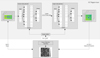 |
Fig. 2 Schematic diagram of our framework. The input dimension of the network corresponds to the state dimension in reinforcement learning, which is defined by the combination of the current parameters and the performance metrics of the surrounding four parameters. The output represents the parameter transformation space, with its dimension corresponding to the action space. |
Design of the DQN.
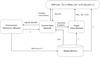 |
Fig. 3 Schematic diagram of the training and deployment procedure of the DQN-based AI supervisor. |
2.4 Application of the AI supervisor to process real observation images
This subsection explores the application of our framework to real observation images, with particular emphasis on source detection and photometry, which are critical components for time domain astronomy research. In real applications, the process involves initially detecting celestial objects followed by photometry of these detected targets. Subsequently, the resulting light curves serve as input for classification algorithms, enabling the identification of potentially interesting celestial phenomena. The variable nature of observational conditions presents significant challenges in parameter optimisation for both detection and photometric tasks. These challenges necessitate sophisticated data processing methodologies to ensure reliability in further scientific study (Wang et al. 2024). Parameter fine-tuning for source detection and photometry algorithms represents a particularly crucial aspect of this process. Our discussion in this subsection demonstrates the method to apply our proposed AI supervisor in addressing these challenges.
Both of these two AI supervisors employed in source detection and photometry tasks comprise training and deployment stages. For the source detection task, we initially generated simulated images based on observational strategies and instrumental characteristics, then determined F1-scores across parameter spaces of the detection algorithm using grid-search method. The source detection AI supervisor underwent training with these simulated images, their associated F1-scores, and ground-truth catalogues, continuously optimising algorithm parameters through a reward feedback mechanism. For the photometry algorithm task, we similarly generated simulated images and extracted sub-images of celestial objects to create the training dataset. The photometry AI supervisor was trained using these sub-images paired with their corresponding magnitude values to fine-tune the aperture size. Leveraging the known magnitudes from simulated data, the AI supervisor iteratively refined the photometry algorithm parameters to minimise measurement error according to input images.
In the deployment stage of our framework, we initially employed the AI supervisor to manage the source detection algorithm for celestial object detection. Given that our available data consists solely of catalogues corresponding to observation images, and considering the potential presence of optical transients, we used KL divergence and the catalogue-derived star count (based on observation mode) as reward metrics. The AI supervisor subsequently fine-tuned the source detection algorithm’s parameters to maximise these rewards. After multiple iterations, the detection algorithm converged on optimal parameters for celestial object detection. During the detection procedure, we implemented fixed-aperture photometry to determine the magnitudes of detected targets. After we detected these celestial objects, we cross-matched these celestial objects with catalogue to obtain reference star positions. These reference stars serve as calibration sources for the photometry algorithm’s AI supervisor. The AI supervisor for photometry uses the differential between catalogue magnitudes and measured magnitudes obtained by the photometry algorithm as its reward function. Through this mechanism, the supervisor optimised the size of the apertures for fixed-aperture photometry to accurately determine magnitudes across all detected targets.
Characteristic parameters of the telescope used in the GWAC.
3 Performance evaluation of the Al supervisor
In this section, we will test the performance of the AI supervisor with two scenarios: one scenario with simulated images and one scenario with real observation images. Both scenarios examine images obtained from wide-field small-aperture telescopes, which are distinguished by pixel scales that exceed the Full Width Half Magnitude of the seeing disc and aperture diameters smaller than 1 meter. The Ground-based Wide-Angle Cameras array (GWAC) (Han et al. 2021) represents a prime example of such wide-field small-aperture telescopic systems employed in our investigation. Details about the telescope are shown in Table 2. The telescopes in the GWAC feature an aperture of 18 cm and a pixel scale of 11.7 arcsec/pixel. These images are acquired with an exposure time of 10 seconds, with one camera obtaining thousands of images each night. Since the GWAC is used to capture optical counterparts of high-energy events, it necessitates real-time processing for target identification, making it an ideal setting for applying our method. To comprehensively evaluate the performance of our approach, the first scenario will solely use simulated images for training and validating the AI supervisor. The ability to easily modify the observational conditions of these images enables thorough validation of our method’s efficacy. In the second scenario, we will incorporate both simulated images and real observation images to train the agent, subsequently deploying it to process real observational images to demonstrate the effectiveness of our approach. The details of these two scenarios will be elaborated upon in the following subsections.
3.1 Performance evaluation of the AI supervisor with simulated images
This section will evaluate the performance of the AI supervisor using simulated observation images. As the observation conditions will vary across different images, we will take into account the following variations in observation conditions:
PSFs: The PSFs of ground-based telescopes are significantly influenced by atmospheric turbulence, resulting in images exhibiting varying Full Width at Half Maximum (FWHM) values. Consequently, we delineate a FWHM range from 0.5 to 3.0 arcseconds, which we segment into five equally spaced intervals to account for different levels of blurring.
Readout noise: Readout noise is primarily caused by temperature variations within the camera, which diminishes the algorithm’s ability to detect dim targets. To simulate images with varying levels of noise, we categorise readout noise into three distinct ranges: 0–5 e−1, 5–15 e−1, and 15–25 e−1. Detail values will be a random variables equally distributed around the above three ranges.
Sky background level: The brightness of the sky background varies under different observational conditions, a phenomenon known as background brightness. To account for the various levels of brightness, we classify background brightness into three distinct categories: 16–18 magnitudes, 18–20 magnitudes, and 20–22 magnitudes.
Celestial object density: Celestial object density refers to the concentration of objects present within the image. To explore various distributions, we classify density into four distinct levels: 3 × 10⁴, 6 × 10⁴, 8 × 10⁴, and 1 × 10⁵ stars per square arcminute.
Distribution of Stars with Different Magnitudes: The distribution of stars across various magnitudes is influenced by the slopes of histograms representing stars of differing magnitudes. To model varying proportions of bright and faint stars, we classify the slopes of these categories into four distinct levels: 0.1, 0.2, 0.3, and 0.4.
Given that the aforementioned variations encompass the majority of observational conditions, we employed images generated from these parameter sets not only to train and validate our method in the first scenario but also to facilitate its training as prior information for real data processing in the second scenario. With the previously defined range of observation parameters, we generated images along with their corresponding catalogues using the SkyMaker. Then, we subsequently employed a grid search method to determine the optimal parameter values for both algorithms: the detection threshold and minimum connected region size for the target-detection algorithm, and the aperture dimension for the photometry algorithm
3.1.1 Performance evaluation of the AI supervisor in the target-detection part with simulated images
Initially, we evaluated the performance of the AI supervisor in the target-detection part. Notably, by solely optimising the detection threshold and minimum connected values, we achieved F1-scores close to the theoretical optimal values. For the majority of images, the deviation from the theoretical optimum was approximately 0.03, demonstrating the effectiveness of our parameter searching approach. We were able to further increase the performance of the source detection with the help from the AI supervisor, however. With these simulated data, we initially trained the AI supervisor for 800 epochs, using the hyper-parameters outlined in Sect. 2.3. This training process has used approximately three hours on a computer equipped with an RTX 4090. The reward convergence curve for the entire training phase is presented in Fig. 4.
The blue curve illustrates the reward value at each step, while the yellow curve depicts the average reward value across each episode. An episode refers to a complete sequence of interactions between the agent and its environment, beginning with an initial state and continuing until a terminal state is reached. In contrast to supervised learning algorithms or unsupervised learning algorithms, AI supervisor does not adjust based on a pre-defined loss function; instead, it employs a reward mechanism to update the network with the objective of maximising cumulative rewards. Initially, during the training phase, the reward value is negative, signifying that the detection algorithm has yet to identify the optimal parameters. As training progresses, the reward value increases, ultimately stabilising after 300 epochs. Given the abstract nature of rewards defined in reinforcement learning algorithm, we used the number of steps required to find the optimal parameters in the target-detection algorithm as an evaluation metric, defining optimal parameters as those which yield an F1-score reaching the predetermined ideal value. As indicated in Fig. 5, more than 10 steps are needed to determine the optimal parameters when we start to train the AI supervisor. After 300 epochs, however, the AI supervisor is able to identify the optimal parameters in about 5 steps, leading to a considerable enhancement in operational efficiency in practical applications, which indicates that our method could be effective in processing real observation data, with the help of its generalisation ability.
We further generated an additional 720 images by systematically varying observation parameters to rigorously evaluate our proposed method. This comprehensive testing approach enabled us to assess performance of the AI supervisor in deployment stage. In this process, we only used the observation conditions and the catalogue within the field of view as prior information, and we defined the reward function according to the approach outlined in Eq. (4). The number of steps taken by the AI supervisor to identify the optimal parameters is illustrated in Fig. 6. The figure indicates that the AI supervisor generally requires fewer than 12 steps to ascertain the best parameters, with the majority of cases falling within the range of 6 to 8 steps. This result emphasises the model’s generalisation ability in detecting celestial objects across diverse conditions, thereby validating its applicability in processing real observation images during the deployment stage.
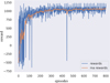 |
Fig. 4 Reward convergence during the network-training stage. |
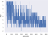 |
Fig. 5 Number of steps for finding the optimal parameters for the detection part during the training stage. |
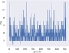 |
Fig. 6 Number of steps required to find the optimal parameters in the detection part for 720 test images. |
3.1.2 Performance evaluation of the AI supervisor in the photometry part with simulated images
Following target detection, we extracted stamp images of celestial objects and performed photometry on each individual object. Wide-field small-aperture telescopes, characterised by their limited aperture size and brief exposure times, typically yield stamp images containing single celestial objects, allowing fixed-aperture photometry to produce reliable measurements. Given these operational constraints, we applied the AI supervisor to optimise the aperture size for fixed-aperture photometry. This approach enables adaptive parameter selection based on image characteristics rather than relying on predetermined settings. Using the dataset and hyper-parameters previously described, we trained the AI supervisor over 2000 epochs. Fig. 7 illustrates the reward convergence curve throughout this training process, demonstrating the progressive improvement of the system’s decision-making capabilities regarding optimal aperture selection.
In Fig. 7, we can find that during early training stage, the AI supervisor has frequently received negative rewards, indicating that initial photometric parameter selections has produced substantial errors. As training advanced, the system has progressively refined its strategy, resulting in steadily increasing reward values until stabilising at approximately 1500 epochs, suggesting successful convergence of the AI supervisor. For a more concrete demonstration of optimisation effectiveness, Fig. 8 displays the evolution of photometry errors obtained by the AI supervisor throughout the training procedure. The horizontal axis tracks training epochs while the vertical axis represents photometry error. Initially selecting parameters with larger errors, the AI supervisor has gradually refined its selections as training progressed, demonstrating the reinforcement learning model’s capacity to adapt and optimise photometric parameters effectively. Following the 1500th epoch, difference between photometry parameters has stabilised consistently below 0.1, indicating that the AI supervisor could maintain high accuracy in parameter selection during subsequent training iterations. These results provide compelling evidence for the effectiveness of the AI supervisor in optimising parameters in photometry part, showing how the system successfully evolved from poor initial performance to consistently accurate parameter selection.
To assess the efficacy of the AI supervisor in optimising photometric parameters, we conducted a comparative analysis against SExtractor’s built-in automatic aperture photometry method, using 1500 simulated images of celestial objects generated by SkyMaker. Fig. 9 (upper panel) displays the photometric error distributions for both methods. The results indicate that the AI supervisor, with RL-optimised aperture parameters, exhibits errors primarily constrained between −0.02 and +0.02 magnitudes. In contrast, SExtractor’s automatic aperture photometry displays a broader error range, extending from −0.5 to +0.5 magnitudes. This discrepancy highlights a substantial improvement in photometric accuracy achieved by the AI supervisor. The lower panel of Fig. 9 presents a histogram quantifying the number of stars at various photometric errors. As demonstrated in this panel, the AI supervisor concentrates photometric errors within a narrower range, confirming its enhanced capability for high precision photometry.
Noise parameters for different simulation levels.
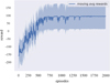 |
Fig. 7 Reward of the training episodes for finding photometric parameters. |
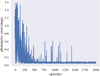 |
Fig. 8 Photometry error during the AI supervisor training procedure. |
3.1.3 Further discussion of the performance of the AI supervisor with simulated images
Before further investigating the performance of the AI supervisor with real observational data, it is essential to demonstrate the factors contributing to the effectiveness of our approach. Firstly, we illustrated the surface of the F1-score and KL for different values of the detection threshold and minimal connected regions across different images in Fig. 10. The images in the upper panel represent simulated images. The images in the middle panel display their corresponding F1-scores and the images in the lower panel display their corresponding KL divergence. As shown in these images, variations in the number, density, and magnitude distribution of stars, along with differing observational conditions, can result in different F1-score surfaces. Nevertheless, these surfaces are smooth, which facilitates an effective search using the AI supervisor proposed in this paper. Moreover, the KL divergence exhibits a distribution similar to that of the F1-Score. Consequently, the KL divergence can serve as a useful reference during the deployment of the AI supervisor.
To comprehensively evaluate the performance and versatility of the AI supervisor across diverse conditions and celestial object fields, we further designed a series of tests incorporating varying levels of noise. Specifically, we introduced different noise levels, including simulated cosmic rays and dead pixels, into the observational images, as detailed in Table 3. The occurrence of cosmic ray strikes and dead pixels follows a Poisson distribution, where the mean of the distribution is determined by the number of such events. The size of a cosmic ray event is defined as the count of adjacent pixels affected, while the intensity is quantified by the greyscale level, exceeding the maximum value found within the images. These artifacts significantly impact detection results; consequently, we prioritised evaluating the AI supervisor’s performance in target-detection part with images heavily corrupted by these effects. The resulting F1-scores for each noise level are presented in Fig. 11. As depicted in the figure, the AI supervisor maintains a consistent F1-score across the range of noise levels tested. This demonstrates the robustness of our AI supervisor to different levels and properties of noises.
To further evaluate the AI supervisor’s performance across diverse celestial fields, we generated simulated images containing varying star densities, as well as images of galaxies. We employed two software packages for this purpose: Stuff for generating catalogues and SkyMaker for creating the simulated images themselves. Using the parameters outlined in Table 4, we generated several catalogues with varying ratios of galaxies to stars. These images served as the basis for testing the detection performance of the AI supervisor in comparison to a source detection algorithm using fixed parameters. The results, presented in Fig. 12, demonstrate that the AI supervisor achieves superior detection performance compared to the algorithm with fixed parameters. This showcases the adaptability of our AI supervisor. However, in cases where the simulated images contain numerous dim stars or extended galaxies, the F1-scores tend to be lower, reflecting the challenge posed by faint or diffuse targets in the evaluation.
We systematically varied image sizes and densities of stars to evaluate the AI supervisor’s performance in both sparse and dense star fields. Source density is controlled by modulating the number of sources per square arcminute. To quantify computational efficiency, we compared the processing time of the fixed-parameter method with that of grid search for parameter optimisation. Furthermore, we restructured the source detection algorithm using CUDA to leverage GPU parallel computing, thereby accelerating image processing (Cao et al. 2025). As shown in Table 5, while the AI supervisor exhibits a slightly longer processing time, it achieves comparable accuracy to grid search, highlighting its advantageous balance of speed and precision. Importantly, the AI supervisor does not need to be executed for every observation image. We propose setting an F1-score threshold for real-time performance evaluation of the source detection algorithm and adjusting parameters only when the F1-score falls below this threshold, optimising efficiency.
To illustrate the procedure for identifying optimal parameters more effectively, we presented a simulated image along with its corresponding F1-Score surfaces and the traces of the AI supervisor in searching for these parameters in Fig. 13. The figure indicates that the AI supervisor guides the parameters towards the bottom-left position, receiving rewards based on the observation conditions and the star catalogue. It is important to highlight, however, that the final position exhibits a slight deviation from the optimal position due to our use of KL divergence and the total number of stars to approximate the F1-Score. In practical applications, calculating the F1-Score necessitates executing the entire pipeline. Furthermore, the presence of new transients not included in the catalogue can adversely affect the F1-Score under these conditions. There is a minor risk that we may not identify the optimal set of parameters, which is a trade-off we must consider in practical applications.
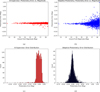 |
Fig. 9 Comparison of the photometry errors in the results obtained by the AI supervisor and those obtained by the automatic aperture photometry in SExtractor. The top two panels show the relation of the photometry error and ground-truth magnitudes obtained by the two methods. The bottom two panels show the histogram of the photometry error obtained by these two methods. |
Parameters for generating the galaxy data.
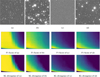 |
Fig. 10 Simulated images generated using various parameters (top panel). The F1-score surface corresponding to these images (middle panel). The bottom panel shows the KL divergence of the corresponding images. |
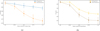 |
Fig. 11 F1-score for images with different properties and noise levels. |
Processing time and F1 score obtained by different methods.
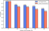 |
Fig. 12 Comparison of the F1-scores of the AI supervisor and the fixed-parameter method for a range of galaxy percentages. |
3.2 Performance evaluation of the method with real observation images
In this section, we evaluated the effectiveness of our method using real observational images. Unlike simulated data, real observational data does not come with known catalogue. Consequently, we first obtained a ground-truth catalogue for these data to validate our method’s effectiveness. We employed the Astrometry (Lang et al. 2010), an open-source astronomical image processing software that automatically identifies and measures celestial coordinates and related information by matching stars in the images with their corresponding celestial positions. Upon successful matching, Astrometry generates a catalogue defined in celestial coordinates. Then we matched these stars with the Gaia DR2 (Gaia Collaboration 2018). The Gaia catalogue allows us to extract essential information of celestial objects, such as the magnitude distribution and the number of all stars in the observation image and magnitudes of reference stars. Through the aforementioned process, we could obtain catalogue for each observational image. The catalogue could further be used to calculate the F1-Score and photometry error.
To determine the optimal parameters as reference for the source detection algorithm and the photometry algorithm, we employed two methods: the grid search method and the genetic algorithm. The grid search method resembles our approach for processing simulated images, where we systematically produced a series of parameters based on predefined grid sizes and scales, allowing for a brute-force search to identify optimal values. Meanwhile, the genetic algorithm is a heuristic approach that searches for optimal parameters within a predefined space by leveraging genetic operations such as mutation and crossover, effectively exploring different parameter sets. We used Geatpy (Holland 1992) to develop an algorithm that identifies optimal parameter sets through genetic algorithms. Using these two methods, we aimed to discover the best parameter sets for the source detection algorithm and the photometry algorithm, with the catalogue obtained above as the benchmark. We stored both the optimal parameters obtained and the number of steps required to achieve them, providing a basis for comparison between the methodologies.
To demonstrate the AI supervisor’s capabilities, we will firstly compare its results with those achieved by human scientists. As discussed in Sect. 2.1, human scientists typically fine-tune the parameters of the source detection algorithm and those of the photometry algorithm using several images as examples. These parameters are then applied to further data processing under the assumption that the subsequent images share similar properties. Consequently, we used several images to fine-tune the parameters of the source detection algorithm and those of the photometry algorithm, applying these as fixed parameters for further data processing. Meanwhile, the AI supervisor is used to search optimal parameter sets for the source detection algorithm and the photometry algorithm. The results are presented in Fig. 14. As illustrated in the figure, the AI supervisor generally achieves a higher F1-Score than human scientists, underscoring the effectiveness of our approach. This figure demonstrates that the AI supervisor achieves the shortest time consumption among the tested methods.
Following the initial test, we proceed to present the results from the second test. This test involves a comparative analysis of detection and photometry results using parameter sets derived through various methods, including the grid search method, the genetic algorithm, and the AI supervisor. The grid search method systematically explores all defined grids across specified scales and steps to identify optimal outcomes. Conversely, the genetic algorithm navigates the parameter space through a heuristic search technique, while our agent refines the optimal parameter set based on prior information. The source-extraction results across these methods are detailed in Table 6. As indicated in the table, both the grid search method and the genetic algorithm typically achieve the highest F1-Scores and the photometry on average, whereas the AI supervisor approach secures a marginally lower F1-Score and photometry accuracy. Nonetheless, it is important to highlight that the AI supervisor requires 241.487 seconds to deliver satisfactory results, making it three times quicker than the genetic algorithm and twenty two times more expedient than the grid search method. Fig. 15 illustrates the comparative time costs of the different methods, underscoring the efficiency of our approach.
After target detection, photometric parameters are individually adjusted for each target with the goal of identifying optimal settings that minimise photometric error, thereby achieving higher measurement accuracy. Fig. 16 presents a comparison between our method and the default automatic aperture photometry provided by SExtractor. As star magnitude increases, photometric error tends to grow. To better illustrate the trend across different magnitudes, a colour gradient is used in the plots. Compared to the default method, our AI-based algorithm is capable of dynamically adjusting the aperture size according to the star’s magnitude, resulting in significantly improved photometric precision. The photometric errors obtained by the AI supervisor are mostly concentrated between 1 and 0.5, indicating a smaller and more stable error range. In contrast, the built-in auto aperture method of SExtractor yields more dispersed errors ranging from 2 to 2, reflecting lower photometric accuracy.
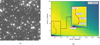 |
Fig. 13 Original observation image (left) and the F1-score surfaces and paths taken by the AI supervisor in searching for the optimal parameters for the detection algorithm (right). |
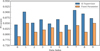 |
Fig. 14 F1-Score of the source detection algorithm with fixed parameters defined by human scientists and those obtained by the AI supervisor. |
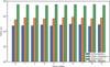 |
Fig. 15 Time required by various methods to obtain optimal parameters for different images. |
Performance comparison of different algorithms.
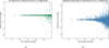 |
Fig. 16 Photometry error distribution after applying the AI supervisor to automatically optimise the SExtractor aperture parameters (panel a). Results of the built-in auto aperture method of SExtractor (panel b). |
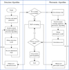 |
Fig. 17 Flowchart of our framework in processing astronomical images for time-domain astronomical observations. |
4 Application of the framework to process real observational data
In earlier sections, we assessed the effectiveness of our approach in processing both simulated and real observational images. Given that the star field and observation conditions may vary for time domain astronomy observations, the AI supervisor must be capable of automatic updates whenever the detection algorithm or the photometry algorithm produces unsatisfactory results. This section will primarily concentrate on the practical application, which encompasses the training, deployment, and real-time oversight of our method. The flowchart depicting our method is illustrated in the Fig. 17.
Generally, there are two modes for deploying the AI supervisor within the data processing pipeline:
Online learning: In this approach, the AI supervisor conducts real-time parameter searches while engaging with the environment, allowing it to adapt to substantial alterations in star field properties or variations in the environment.
Offline prediction: In this mode, when the observational environment is stable or the distribution of star fields remains consistent, the AI supervisor can directly use the previously trained model for predictions without requiring real-time parameter updates.
For application of the AI supervisor in processing time-domain astronomy observation data, we propose the implementation of a hybrid model. Initially, the system operates in an offline learning mode with model trained with simulated data, where we cross-match detected stars against the catalogue provided by Gaia DR2, which is constrained by limited magnitude obtained by the sky background, the pixel scale, the exposure time and the aperture of the telescope. The F1-Score serves as the evaluation criterion for source detection part. After the detection part, we will carry out photometry and use photometry accuracy as the evaluation criterion for the photometry part. If the F1-Score or photometry accuracy experiences a sudden and significant drop during the sequential processing of data, we will infer that the parameters are unstable, prompting a transition to an online learning mode. In this mode, we will employ a reinforcement learning strategy to train the AI supervisor and derive new parameter sets.
Based on the aforementioned method, we conducted tests using a series of observational images captured by a single camera of the GWAC on November 6th. 2024. To illustrate the effectiveness of our algorithm, we selected images with an interval of 1 minutes, as these images could exhibit greater variations. The F1-Score and the photometry accuracy of these images, along with the steps necessitated by our algorithm to identify the optimal parameters, is presented in Fig. 18. This figure demonstrates that our approach can successfully detect variations in the observational environment while identifying optimal parameters, resulting in a higher F1-Score and photometry accuracy compared to the fixed parameters derived from human scientists. In practical applications, if a sudden drop in the F1-Score or photometry accuracy is detected, the AI supervisor will autonomously re-initiate parameter adjustment to search for a new optimal set, ensuring robustness under changing observational conditions.
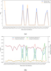 |
Fig. 18 Number of steps used by the AI supervisor to attain optimal parameters for the target-detection part and the photometry part (top). Comparison of the F1-scores and the photometry accuracy achieved using fixed parameters determined by human scientists with those obtained using parameters optimised by the AI supervisor (bottom). |
5 Conclusions and future works
We introduced a reinforcement learning-based AI supervisor designed to adaptively optimise the parameters for astronomical source-extraction algorithms. We conducted a thorough analysis using simulated and real astronomical observation images in a source-detection and photometry task, and we demonstrated that the AI supervisor effectively determined the optimal parameter sets for each task. To facilitate the application of the AI supervisor to real observation data, we developed a source-extraction framework that integrates GPU-accelerated target-detection and photometry algorithms and the AI supervisor. Testing with real observation images revealed that our framework achieves a higher photometric accuracy, a higher detection accuracy, and a higher detection limit automatically. They surpass conventional methods that rely on human-derived parameters. The results underscore that the AI supervisor is a powerful tool for integrating classical and deep-learning-based methods in various astronomical data-processing applications. Its adaptive nature means that it can be dynamically optimised, which enhances the efficiency and accuracy of astronomical data-analysis workflows.
Acknowledgements
This work is supported by the National Key Research and Development Programme with funding numbers 2023YFF0725300, National Natural Science Foundation of China (NSFC) with funding numbers 12173027, 12303105 and 12173062. This work is supported by the Young Data Scientist Project of the National Astronomical Data Center.
References
- Alom, M. Z., Taha, T. M., Yakopcic, C., et al. 2018, arXiv e-prints [arXiv:1803.01164] [Google Scholar]
- Andreon, S., Gargiulo, G., Longo, G., Tagliaferri, R., & Capuano, N. 2000, MNRAS, 319, 700 [Google Scholar]
- Arulkumaran, K., Deisenroth, M. P., Brundage, M., & Bharath, A. A. 2017, IEEE Signal Process. Mag., 34, 26 [Google Scholar]
- Axelrod, T., Connolly, A., Ivezic, Z., et al. 2004, in American Astronomical Society Meeting Abstracts, 205, 108.11 [Google Scholar]
- Bellm, E. C., Kulkarni, S. R., Barlow, T., et al. 2019, PASP, 131, 068003 [Google Scholar]
- Bertin, E., & Arnouts, S. 1996, A&AS, 117, 393 [NASA ADS] [CrossRef] [EDP Sciences] [Google Scholar]
- Beskin, G., Biryukov, A., Gutaev, A., et al. 2023, Photonics, 10, 1352 [Google Scholar]
- Bialek, S., Bertin, E., Fabbro, S., et al. 2024, MNRAS, 531, 403 [Google Scholar]
- Cabrera-Vives, G., Reyes, I., Förster, F., Estévez, P. A., & Maureira, J.-C. 2017, ApJ, 836, 97 [NASA ADS] [CrossRef] [Google Scholar]
- Cao, L., Jia, P., Li, J., et al. 2025, AJ, 169, 215 [Google Scholar]
- Casas, J. M., González-Nuevo, J., Bonavera, L., et al. 2022, A&A, 658, A110 [NASA ADS] [CrossRef] [EDP Sciences] [Google Scholar]
- Castro-Tirado, A. J., Soldán, J., Bernas, M., et al. 1999, A&AS, 138, 583 [NASA ADS] [CrossRef] [EDP Sciences] [Google Scholar]
- Deng, J., Dong, W., Socher, R., et al. 2009, in 2009 IEEE Conf. Comput. Vis. Pattern Recognit., 248 [CrossRef] [Google Scholar]
- Dyer, M. J., Steeghs, D., Galloway, D. K., et al. 2020, in Ground-based and airborne telescopes VIII, 11445, 1355 [Google Scholar]
- Gaia Collaboration 2018, VizieR Online Data Catalog: I [Google Scholar]
- Gal-Yam, A., Ofek, E. O., Poznanski, D., et al. 2006, ApJ, 639, 331 [NASA ADS] [CrossRef] [Google Scholar]
- Gal-Yam, A., Kasliwal, M. M., Arcavi, I., et al. 2011, ApJ, 736, 159 [NASA ADS] [CrossRef] [Google Scholar]
- Girshick, R. 2015, in Proc. IEEE Int. Conf. Comput. Vis., 1440 [Google Scholar]
- Gromadzki, M., Hamanowicz, A., Wyrzykowski, L., et al. 2019, A&A, 622, L2 [NASA ADS] [CrossRef] [EDP Sciences] [Google Scholar]
- Haigh, C., Chamba, N., Venhola, A., et al. 2021, A&A, 645, A107 [NASA ADS] [CrossRef] [EDP Sciences] [Google Scholar]
- Han, X., Xiao, Y., Zhang, P., et al. 2021, PASP, 133, 065001 [NASA ADS] [CrossRef] [Google Scholar]
- Han, K., Wang, Y., Chen, H., et al. 2022, IEEE Trans. Pattern Anal. Mach. Intell., 45, 87 [Google Scholar]
- He, K., Gkioxari, G., Dollár, P., & Girshick, R. 2017, in Proc. IEEE Int. Conf. Comput. Vis., 2961 [Google Scholar]
- He, Z., Qiu, B., Luo, A.-L., et al. 2021, MNRAS, 508, 2039 [NASA ADS] [CrossRef] [Google Scholar]
- Holland, J. H. 1992, Adaptation in Natural and Artificial Systems: An Introductory Analysis with Applications to Biology, Control, and Artificial Intelligence (MIT press) [Google Scholar]
- Ivezić, Ž., Kahn, S. M., Tyson, J. A., et al. 2019, ApJ, 873, 111 [Google Scholar]
- Jia, P., Sun, R., Wang, W., Cai, D., & Liu, H. 2017, MNRAS, 470, 1950 [Google Scholar]
- Jia, P., Liu, Q., & Sun, Y. 2020, AJ, 159, 212 [NASA ADS] [CrossRef] [Google Scholar]
- Jia, P., Wang, W., Ning, R., & Xue, X. 2022, Opt. Express, 30, 21362 [Google Scholar]
- Jia, P., Jia, Q., Jiang, T., & Yang, Z. 2023a, Astron. Comput., 44, 100732 [Google Scholar]
- Jia, P., Zheng, Y., Wang, M., & Yang, Z. 2023b, Astron. Comput., 42, 100687 [Google Scholar]
- Jia, P., Jia, Q., Jiang, T., & Liu, J. 2023c, AJ, 165, 233 [Google Scholar]
- Jiang, P., Ergu, D., Liu, F., Cai, Y., & Ma, B. 2022, Procedia Comput. Sci., 199, 1066 [Google Scholar]
- Kaiser, N. 2004, in Ground-based Telescopes, 5489, 11 [Google Scholar]
- Kou, S. 2019, in AOPC 2019: Space Optics, Telescopes, and Instrumentation, 11341, 99 [Google Scholar]
- Lang, D., Hogg, D. W., Mierle, K., Blanton, M., & Roweis, S. 2010, AJ, 139, 1782 [Google Scholar]
- Law, N. M., Corbett, H., Galliher, N. W., et al. 2022, PASP, 134, 035003 [Google Scholar]
- Liu, J., Soria, R., Wu, X.-F., Wu, H., & Shang, Z. 2021, An. Acad. Bras. Cienc., 93 [Google Scholar]
- Lokhorst, D. M., Abraham, R. G., van Dokkum, P., & Chen, S. 2020, in Ground-based and Airborne Telescopes VIII, 11445, 492 [Google Scholar]
- Masci, F. J., Laher, R. R., Rusholme, B., et al. 2018, PASP, 131, 018003 [Google Scholar]
- Mirjalili, S., & Mirjalili, S. 2019, Evol. Algorithms Neural Netw.: Theory Appl., 43 [Google Scholar]
- Myers, A. D., Moustakas, J., Bailey, S., et al. 2023, AJ, 165, 50 [NASA ADS] [CrossRef] [Google Scholar]
- Nousiainen, J., Rajani, C., Kasper, M., et al. 2022, A&A, 664, A71 [NASA ADS] [CrossRef] [EDP Sciences] [Google Scholar]
- Osband, I., Blundell, C., Pritzel, A., & Van Roy, B. 2016, Adv. Neural Inf. Process. Syst., 29 [Google Scholar]
- Panes, B., Eckner, C., Hendriks, L., et al. 2021, A&A, 656, A62 [NASA ADS] [CrossRef] [EDP Sciences] [Google Scholar]
- Poole, D. L., & Mackworth, A. K. 2010, Artificial Intelligence: Foundations of Computational Agents (Cambridge University Press) [CrossRef] [Google Scholar]
- Rau, A., Kulkarni, S. R., Law, N. M., et al. 2009, PASP, 121, 1334 [NASA ADS] [CrossRef] [Google Scholar]
- Ren, S., He, K., Girshick, R., & Sun, J. 2015, Adv. Neural Inf. Process. Syst., 28 [Google Scholar]
- Rezaei, S., McKean, J. P., Biehl, M., & Javadpour, A. 2022, MNRAS, 510, 5891 [NASA ADS] [CrossRef] [Google Scholar]
- Rix, H.-W., Barden, M., Beckwith, S. V., et al. 2004, ApJS, 152, 163 [CrossRef] [Google Scholar]
- Russakovsky, O., Deng, J., Su, H., et al. 2015, Int. J. Comput. Vis., 115, 211 [Google Scholar]
- Silver, D., Huang, A., Maddison, C. J., et al. 2016, Nature, 529, 484 [CrossRef] [PubMed] [Google Scholar]
- Steeghs, D., Galloway, D., Ackley, K., et al. 2022, MNRAS, 511, 2405 [NASA ADS] [CrossRef] [Google Scholar]
- Stoppa, F., Bhattacharyya, S., de Austri, R. R., et al. 2023, A&A, 680, A109 [NASA ADS] [CrossRef] [EDP Sciences] [Google Scholar]
- Sun, R.-y., Yu, P.-p., & Zhang, W. 2022, Adv. Space Res., 70, 2315 [Google Scholar]
- Sun, R., Jia, P., Sun, Y., et al. 2023, AJ, 166, 235 [Google Scholar]
- Tonry, J., Denneau, L., Heinze, A., et al. 2018, PASP, 130, 064505 [NASA ADS] [CrossRef] [Google Scholar]
- Turing, A. 2004, Intelligent Machinery (1948), ed. B. Jack Copeland, 395 [Google Scholar]
- Udalski, A., Szymański, M. K., & Szymański, G. 2015, arXiv e-prints [arXiv:1504.05966] [Google Scholar]
- Wang, Y., Sun, R., Deng, T., et al. 2024, RAA, 24, 075012 [Google Scholar]
- Watkins, C. J., & Dayan, P. 1992, Mach. Learn., 8, 279 [Google Scholar]
- Xu, Y., Xin, L., Wang, J., et al. 2020, PASP, 132, 054502 [Google Scholar]
- Yatawatta, S. 2023, arXiv e-prints [arXiv:2301.03933] [Google Scholar]
- Yatawatta, S. 2024, Astron. Comput., 48, 100833 [Google Scholar]
- Yatawatta, S., & Avruch, I. M. 2021, MNRAS, 505, 2141 [NASA ADS] [CrossRef] [Google Scholar]
- Zhan, Y., Jia, P., Xiang, W., & Li, Z. 2022, in Modeling, Systems Engineering, and Project Management for Astronomy X, 12187, 756 [Google Scholar]
- Zhang, M., Jia, P., Li, Z., et al. 2023, Opt. Express, 31, 44054 [Google Scholar]
All Tables
All Figures
|
Fig. 1 Two-dimensional heat map representing the parameter distribution of the detection threshold (DETECT_THRESH) and the minimally connected regions (DETECT_MINAREA) for the target-detection task in a specific image, thus providing a visual depiction of the state distribution. The depiction of the designed states and actions is presented in the left panel. The current parameter position is denoted as (i, j), and the four adjacent positions are identified as (i+1, j), (i-1, j), (i, j+0.1), and (i, j-0.1). |
| In the text | |
|
Fig. 2 Schematic diagram of our framework. The input dimension of the network corresponds to the state dimension in reinforcement learning, which is defined by the combination of the current parameters and the performance metrics of the surrounding four parameters. The output represents the parameter transformation space, with its dimension corresponding to the action space. |
| In the text | |
|
Fig. 3 Schematic diagram of the training and deployment procedure of the DQN-based AI supervisor. |
| In the text | |
|
Fig. 4 Reward convergence during the network-training stage. |
| In the text | |
|
Fig. 5 Number of steps for finding the optimal parameters for the detection part during the training stage. |
| In the text | |
|
Fig. 6 Number of steps required to find the optimal parameters in the detection part for 720 test images. |
| In the text | |
|
Fig. 7 Reward of the training episodes for finding photometric parameters. |
| In the text | |
|
Fig. 8 Photometry error during the AI supervisor training procedure. |
| In the text | |
|
Fig. 9 Comparison of the photometry errors in the results obtained by the AI supervisor and those obtained by the automatic aperture photometry in SExtractor. The top two panels show the relation of the photometry error and ground-truth magnitudes obtained by the two methods. The bottom two panels show the histogram of the photometry error obtained by these two methods. |
| In the text | |
|
Fig. 10 Simulated images generated using various parameters (top panel). The F1-score surface corresponding to these images (middle panel). The bottom panel shows the KL divergence of the corresponding images. |
| In the text | |
|
Fig. 11 F1-score for images with different properties and noise levels. |
| In the text | |
|
Fig. 12 Comparison of the F1-scores of the AI supervisor and the fixed-parameter method for a range of galaxy percentages. |
| In the text | |
|
Fig. 13 Original observation image (left) and the F1-score surfaces and paths taken by the AI supervisor in searching for the optimal parameters for the detection algorithm (right). |
| In the text | |
|
Fig. 14 F1-Score of the source detection algorithm with fixed parameters defined by human scientists and those obtained by the AI supervisor. |
| In the text | |
|
Fig. 15 Time required by various methods to obtain optimal parameters for different images. |
| In the text | |
|
Fig. 16 Photometry error distribution after applying the AI supervisor to automatically optimise the SExtractor aperture parameters (panel a). Results of the built-in auto aperture method of SExtractor (panel b). |
| In the text | |
|
Fig. 17 Flowchart of our framework in processing astronomical images for time-domain astronomical observations. |
| In the text | |
|
Fig. 18 Number of steps used by the AI supervisor to attain optimal parameters for the target-detection part and the photometry part (top). Comparison of the F1-scores and the photometry accuracy achieved using fixed parameters determined by human scientists with those obtained using parameters optimised by the AI supervisor (bottom). |
| In the text | |
Current usage metrics show cumulative count of Article Views (full-text article views including HTML views, PDF and ePub downloads, according to the available data) and Abstracts Views on Vision4Press platform.
Data correspond to usage on the plateform after 2015. The current usage metrics is available 48-96 hours after online publication and is updated daily on week days.
Initial download of the metrics may take a while.