| Issue |
A&A
Volume 699, July 2025
|
|
|---|---|---|
| Article Number | A67 | |
| Number of page(s) | 14 | |
| Section | Planets, planetary systems, and small bodies | |
| DOI | https://doi.org/10.1051/0004-6361/202453069 | |
| Published online | 01 July 2025 | |
The atmospheres of rocky exoplanets
III. Using atmospheric spectra to constrain surface rock composition
Institute for Astronomy (IfA), University of Vienna,
Türkenschanzstrasse 17,
1180
Vienna,
Austria
★ Corresponding author: This email address is being protected from spambots. You need JavaScript enabled to view it.
Received:
19
November
2024
Accepted:
12
May
2025
Abstract
Context. The crust composition of rocky exoplanets with substantial atmospheres cannot be observed directly. However, recent developments have enabled novel observations and characterisations of their atmospheres.
Aims. We aim to establish a link between observable spectroscopic atmospheric features and the mineralogical crust composition of exoplanets. This enables us to constrain the surface composition simply by observing the transit spectra.
Methods. We used a diverse set of total element abundances inspired by various rock compositions, Earth, Venus, and CI chondrite as a basis for our bottom-to-top atmospheric model. We assumed thermal and chemical equilibrium between the atmosphere and the planetary surface. Based on the atmospheric models in hydrostatic and chemical equilibrium, with the inclusion of element depletion due to cloud formation, we calculated the theoretical transit spectra.
Results. The atmospheric type classification allows us to constrain the surface mineralogy, especially with respect to sulphur compounds, iron oxides and hydroxides, feldspars, silicates, and carbon species. Spectral features offer an opportunity to differentiate among the atmospheric types, allowing for a number of constraints to be placed on the surface composition.
Key words: astrochemistry / planets and satellites: atmospheres / planets and satellites: composition / planets and satellites: surfaces / planets and satellites: terrestrial planets
© The Authors 2025
 Open Access article, published by EDP Sciences, under the terms of the Creative Commons Attribution License (https://creativecommons.org/licenses/by/4.0), which permits unrestricted use, distribution, and reproduction in any medium, provided the original work is properly cited.
This article is published in open access under the Subscribe to Open model. This email address is being protected from spambots. You need JavaScript enabled to view it. to support open access publication.
1 Introduction
There are currently over 7000 known exoplanets1, with a significant percentage made up by terrestrial worlds. Revealing a broad range of planetary parameters (e.g. radius, mass, density, temperature, etc) indicating a diverse set of atmospheric, surface, and interior compositions (e.g. Noack & Breuer 2014; Leconte et al. 2015; Grenfell et al. 2020; Lichtenberg et al. 2022; Lichtenberg & Miguel 2025). While characterising atmospheres and surfaces of rocky exoplanets is one of the driving questions in modern astrophysics (e.g. Byrne et al. 2024, especially in the context of the Astro2020 Decadal Survey (National Academies of Sciences, Engineering, and Medicine 2021) as well as the upcoming European Space Agency’s ESA Voyage 2050 (Quanz et al. 2021; Janson et al. 2022; Rossi et al. 2022), its direct observation is challenging at best and, for many planets, even impossible. On the one hand, for airless bodies, the geological composition can, in principle, be constrained by reflected and emitted light (e.g. Madden & Kaltenegger 2018; Asensio Ramos & Pallé 2021; Alei et al. 2024; Hammond et al. 2025) as well as polarimetry (e.g. Rossi & Stam 2017, 2018). On the other hand, for planets with a substantial atmosphere, the link between the observables in the atmosphere (absorption from molecules, effects of aerosols from clouds and hazes, etc) needs to be understood. The chemical composition of the atmosphere can be indicative of the planetary interior and surface (e.g. Schaefer et al. 2012; Herbort et al. 2020; Ortenzi et al. 2020; Timmermann et al. 2023; Baumeister & Tosi 2023; Seidler et al. 2024). Furthermore, the cloud composition present in a planetary atmosphere obstruct the view to the surface itself (Kreidberg et al. 2014; Helling 2022); however, it can, in principle, be used in order to constrain surface conditions (e.g. Loftus et al. 2019; Herbort et al. 2022).
Exoplanets, along with their atmospheres, surfaces, and interiors, are expected to be much more diverse than what is known from the terrestrial planets in the Solar System (Grenfell et al. 2020). The secondary atmospheres of rocky exoplanets is a result of outgassing over planetary timescales. The composition of the outgassed material itself is diverse (Guimond et al. 2023) and connected to the mantle composition, which drives the outgassing (Ortenzi et al. 2020; Guimond et al. 2021; Baumeister et al. 2023; Guimond et al. 2024). In particular, the redox state of the mantle can generally influence the volatile composition which is outgassed (Gaillard et al. 2021, 2022). The outgassed material can be used to constrain the planetary interior (Spaargaren et al. 2020). Besides the presence of a given condensate species itself, their abundances can also largely vary from planet to planet; in particular, the amount of water present ranges from trace amounts to thick water envelopes (e.g. Kite & Schaefer 2021; Kimura & Ikoma 2022; Rogers et al. 2025). In addition, other volatiles such as sulphur are being investigated (Janssen et al. 2023; Lodders & Fegley 2024).
For the investigation of the mineralogical and near-crust atmospheric composition, a chemical phase equilibrium between these two is often assumed (e.g. Miguel et al. 2011; Schaefer et al. 2012; Kite et al. 2016; Herbort et al. 2020). Particularly in the case of hot, rocky exoplanets, the atmosphere can be composed of vaporised rock (e.g. van Buchem et al. 2023; Zilinskas et al. 2023). Additionally to these theoretical investigations, complementary works of vaporising rocks have been done in the laboratory (Thompson et al. 2021, 2023). The atmospheric elemental composition is also affected by cloud formation (e.g. Ackerman & Marley 2001; Mbarek & Kempton 2016; Herbort et al. 2022; Helling 2022).
Recent observations with the James Webb Space Telescope (JWST) (Gardner et al. 2023) are providing the first indications for the detection of the atmosphere on the rocky planet 55 Cnc e (Hu et al. 2024). However, observations of smaller planets, such as LHS 475b (Lustig-Yaeger et al. 2023), TRAPPIST 1b (Greene et al. 2023), TRAPPIST 1c (Zieba et al. 2023), and GJ 1132b (Xue et al. 2024). do not show any conclusive evidence that an atmosphere has been detected; instead, they remain consistent with airless bodies. Future instruments on the next generation of telescopes, such as the Extremely Large Telescope (ELT) (Gilmozzi & Spyromilio 2007), and space missions such as PLATO (Rauer et al. 2025), Ariel (Tinetti et al. 2018), Habitable Worlds Observatory (HWO)2, and Large Interferometer For Exoplanets (LIFE Quanz et al. 2022) will further enhance the capabilities of the detection of atmospheres of Earth-sized planets.
The detection of atmospheres of rocky planets has some major complications. Firstly, the contrast from planet to star is small and best for low-mass stars. Secondly, the atmosphere of the planet has to be retained; especially in the case of planets around low-mass stars, this is unlikely due to the proximity to the host star and the resulting atmospheric loss (e.g. Van Looveren et al. 2024, 2025). Thirdly, the entirety of the atmosphere is not detectable, as the atmospheres become optically thick for high pressures and at higher altitudes if clouds or hazes are present.
To further understand the connection between the observable parts of the atmosphere and the surface composition, we investigated a diverse set of total element abundances, whose resulting atmospheric compositions cover a diverse range of atmospheric compositions (see Woitke et al. 2021). The basis for the atmospheric model used in this work is a bottom-to-top equilibrium chemistry model. The near-crust atmosphere is in chemical phase equilibrium with the surface (Herbort et al. 2020) and throughout the atmosphere, the elemental depletion due to the removal of thermally stable cloud condensates is considered (see also Herbort et al. 2022). Based on these atmospheres, we create theoretical transmission spectra to bridge potential observables to surface compositions.
At this point, it needs to be noted that the assumption of chemical and phase equilibrium between the atmosphere and crust is a limiting factor for the models presented throughout this work. In the specific case of the moderately low temperatures investigated here, the systems may not reach the theoretically favourable equilibrium state. Causes for this out-of-equilibrium state may be an atmospheric composition driven by volcanic activity or photochemistry. The gases released from volcanic outgassing may be in equilibrium at the outgassing temperatures, but the timescales for cooling down to the surrounding atmospheric temperature are governed by kinetic chemistry; for the equilibration to low temperatures, these timescales might be too long to be relevant. Therefore, systems with atmospheres dominated by active volcanism and temperatures of T < 700 K might not reach the equilibrium state (Liggins et al. 2023). However, given enough geological inactive time, the system of atmosphere and surface composition should evolve towards the chemical equilibrium. However, for modest outgassing rates, the main atmospheric components can also be described in chemical phase equilibrium. Although Earth experiences volcanism and further effects such as biological activity, an equilibrium model similar to those presented in this paper can be constructed, which only deviates in molecules with number densities of less than 5 ppm. In particular, this includes CH4, which is not stable in the equilibrium model (see Appendix A in Herbort et al. 2022).
The equilibration of the condensate phase depends on the timescales of condensation directly form the gas phase as well as the rearrangement (annealing) of the condensate phase itself. An approximation of these timescales for different rocks is also discussed in Herbort et al. (2020). However, the temperature threshold for assuming chemical equilibrium remains unknown. Understanding the modelling results with this in mind, provides an insight to potential links present in understanding the atmospheric crust and ultimately atmospheric interior link for the diversity of rocky exoplanets (see also Byrne et al. 2024).
Investigations of deviations from this equilibrium state are beyond the scope of this work and will be investigated in the future. A further important aspect to be noted here is photochemistry, which drives the system out of chemical equilibrium to a different stable state. However, the compositions of this stable state are not only dependent on the atmospheric composition, but especially on the incoming stellar radiation. This can lead to the depletion of species such as H2O, CH4, or NH3 with respect to their expected presence in chemical equilibrium (see e.g. Kasting 1982; Rugheimer et al. 2015; Hu 2021). However, the degree to which these species are depleted is highly dependent on stellar irradiation. As this introduces further dimensions to the investigated parameter space, we do not include it in the work at hand, as the main focus is the investigation of the changes in surface and atmospheric composition induced by differences in total elemental composition.
The nature of chemical equilibrium solvers enables the investigation of a model that includes many more species compared to chemical kinetics; whereas photochemical networks are due to computational constraints mostly limited to a network based on a limited number of elements, mostly limited to a subset of CHNOPS elements (compare to e.g. Rimmer & Helling 2016; Tsai et al. 2021; Lee et al. 2024). As the effect of photochemistry varies strongly with the incoming stellar radiation and the atmospheric composition, their inclusion expands the potential parameter space significantly. Therefore, investigating the effects of photochemistry on the atmospheric composition and atmospheric types in general is beyond the scope of this work.
In Sect. 2, we provide an overview of our atmospheric and crust modelling methods, give an overview of the atmospheric classification scheme, and introduce the model-transmission spectra generation used in this work. In Sect. 3.1, the diversity of the resulting model atmospheres is shown, in Sect. 3.2, their clouds, and in Sect. 3.3, the resulting crust composition and possible links between certain crust condensates and their atmospheres. Additionally, in Sect. 3.4, we discuss the resulting transmission spectra and their observability. In Sect. 3.5, we describe the peculiarities of graphite as a stable condensate at low pressures. Section 4 summarises and discusses the implications of our findings.
2 Methods
In this section, we briefly describe our atmospheric model (Sect. 2.1), before introducing the parameter space for the atmospheric diversity (Sect. 2.2). Afterwards, we describe how the transmission spectra were created (Sect. 2.3).
2.2 Atmospheric and crust modelling
For the modelling of atmospheric and crust compositions, we used the equilibrium chemistry code GGCHEM (Woitke et al. 2018). Based on a given set of total element abundances, a given pressure, and a given temperature, the chemical and phase equilibrium was solved. Based on the atmosphere-crust interaction layer (see also Herbort et al. 2020), we built a bottom-to-top atmosphere with chemical and phase equilibrium at each layer (see also Herbort et al. 2022). The gas phase elemental composition was used as the total element abundance in the atmospheric layer above. Thus, all thermally stable condensates (liquid and solid) are forming and deplete the effected elemental abundances in the atmospheric layers above. At the base layer, all thermally stable solid and liquid condensates represent the crust composition. The different sets of total element abundances are based on a total of 18 elements (H, C,N, O, F, Na, Mg, Al, Si, P, S, Cl, K, Ca, Ti, Cr, Mn, and Fe), which can form a total of 474 gas phase species and 213 condensates, with 40 liquids thereof. Throughout this work, we used a parametrised pressure and temperature (p, T)-profile as introduced in the following and a range of different total element abundances, reflecting a variety of different surface and atmosphere compositions.
We based our atmospheric model on the polytropic atmospheric model used in Herbort et al. (2022). However, as we investigate the transmission spectra, it is necessary to model to higher parts of the atmosphere. In this work, we defined the top of our model atmosphere as 10−7 bar. A purely polytropic atmosphere for a pressure change of seven orders of magnitude is trending towards T = 0 K, which is not an accurate portrayal for realistic atmospheres. Therefore, we introduced a modified (p, T)-structure,
 (1)
(1)
with the introduction of a shift pressure, pshift. Furthermore, we used a surface temperature, Tsurf, surface pressure, psurf, and the polytropic exponent, κ = (γ - 1)/γ, where γ is the polytropic index. We defined the shift pressure as
 (2)
(2)
where χ is given by the ratio of the surface temperature and a minimum temperature Tmin as
 (3)
(3)
We note that due to this shift, the parameters γ and κ are not equivalent to the polytropic parameters determined by heat capacities; instead, the parameters are similar in nature, but display different values.
In reality, the composition of the atmosphere and condensation of cloud condensates can strongly influence the (p, T)-structure, due to various heating and cooling effects, including the absorption of stellar radiation and the release of latent heat during condensation. However, to investigate the effects caused by purely changing the base composition, we kept the (p, T)-profile consistent for different compositions.
For the grid of (p, T)-profiles, we adopted Tmin = 0.75 · Tmax and κ = 0.9 for all our model atmospheres. Additionally we define four surface temperatures with Tsurf = Tmax at 300 K, 400 K, 500 K, and 600 K. Examples for the resulting atmospheric profiles can be seen in Fig. 1 in comparison to Earth’s atmospheric profile.
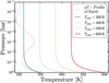 |
Fig. 1 Comparison of our atmospheric profile model for Tsurf = 300 K, 400 K, 500 K, 600 K, Tmin = 0.75 · Tsurf, and κ = 0.9 in comparison to Earth’s atmospheric profile. |
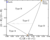 |
Fig. 2 Parameter space for CHNO element abundances based on Woitke et al. (2021). Solar System rocky bodies atmospheres are indicated with a star. The different atmospheric types defined by the presence of different molecules (see Eq. (4)) are also indicated. |
2.2 Atmospheric diversity
The atmospheric compositions of rocky exoplanets are expected to be more diverse than the compositions present in planets in the solar system. Woitke et al. (2021) introduced a scheme to characterise the atmospheric composition based on the abundance of the most important chemical elements (C, H, N, and O). This results in four distinct atmospheric types in chemical equilibrium:
 (4)
(4)
In Fig. 2, we show this CHO parameter space for a fixed N content. In addition, the position of rocky solar system bodies atmospheres is shown. The axes are given by
 (5)
(5)
for the vertical axis and horizontal axis, respectively, providing a clear depiction of the composition of the different atmospheric types.
To cover the parameter space, we investigated different sets of total element abundances, which are given in Table A.1 (cf. Herbort et al. 2020, 2022).
We used various total element abundances, based on bulk silicate earth (BSE, Schaefer et al. 2012), mid-oceanic ridge basalt (MORB, Arevalo & McDonough 2010), continental crust (CC, Schaefer et al. 2012), CI chondrite (CI, Lodders et al. 2009), and Earth-like composition (Herbort et al. 2022). Furthermore, we investigated sets of element abundances fit to the atmospheric composition of Venus (cf. Rimmer et al. 2021).
To fill the parameter space with more diverse atmospheres, we modified some of the described elemental abundances by changing the abundances of certain elements. These changes are described below.
We modified the BSE abundance by adding 20% and 30% of H, C, and O to the initial BSE mass fractions. These models are called BSE20HCO and BSE30HCO, respectively. Furthermore, we added 8% and 15% water to the original BSE abundance as in Herbort et al. (2020), referred to as BSE8 and BSE15 in this work. The resulting mass fractions can be found in Table A.1. An oxygen-rich atmosphere was created based on the MORB abundance by adding 10% mass fraction oxygen. We call the resulting model MORBo.
We explored different water content for the Earth-like model, by reducing the H abundance by 50% and 70% from the initial Earth abundance to form Earth-50 and Earth-70, respectively. Additionally, a ‘dry Earth’ scenario was created by reducing the H and O mass fractions of the initial Earth mass fractions, assuming all H would form water, where only 10% of the water would remain (Earthdry).
The Venus abundances are created in such a way so that they resemble gas-phase element abundances (Rimmer et al. 2021) for the venusNoSurf model (VNS). For a model that portrays the surface more accurately, we added the measurements from Vega 2 (Surkov et al. 1986). These measured references do not include the elements F, P, and Cr, so their abundance was set to 0. Because the surface elements dominate over the atmosphere, we multiplied them by a factor of 1000. The model is then once again adapted to resemble Venus’ atmospheric conditions and referred to as the venusSurf model (VS). We then created two more models based on this model, with 2% and 10% additional water content (venus2 and venus10, respectively).
2.3 Spectrum calculation with ARCiS
For the spectra, the ARtful modelling Code for exoplanet Science (ARCIS) code was used (Min et al. 2020). We input the (p, T)-structure from Sect. 2.1 and the chemical composition calculated by GGCHEM, together with planet size, mass, host star distance, and the stellar size and temperature. The transmission spectrum of the planetary atmosphere was then calculated based on the gas phase opacities.
However, not all molecules present in the gas phase (based on the GGCHEM calculations) have listed opacities available in ARCIS. Additionally, due to computation time limitations, we have had to constrain our compositions to the available and most abundant molecules. To compute the transmission spectra, we included all atmospheric species with peak number densities at a point in the atmosphere of above 10−9 (1 ppb).
The parameters for the investigated planets resemble those of an Earth analogue of Earth’s size and mass. The star-planet distance can be calculated using
 (6)
(6)
with L being the stellar luminosity, σ the Stefan Boltzmann constant, A the planet’s Bond albedo, and T the effective temperature. For the albedo, we took the three rocky planets with an atmosphere of our solar system and the average albedo, yielding A = 0.45. We set the effective temperature T to Tsurf used in the atmospheric modelling.
The star was fixed to an M1-type star with an effective temperature of Teff = 3660 K, M = 0.42 M, and R = 0.5 R. A smaller star would lead to an increased transit depth, for an identical planet, making the observations easier. While this would make late M-dwarfs the ideal host star, it is realistically less likely for rocky planets around late M-dwarfs to retain an atmosphere. This is due to the influence of the XUV on the atmosphere and the proximity of the planet to the host star (e.g. Van Looveren et al. 2024, 2025). Therefore we used an M1 star as the host star for our theoretical transmission spectra.
The exclusion of clouds for the calculation of the transmission spectra provides an ideal case for the transmission spectra, as the spectral depth is not effected under the assumption of a cloud-free case. This choice was motivated by the fact that the major effect of cloud condensation (for the atmospheric (p, T) profiles used in this work) is limited to the lowest part of the atmosphere and may also be subject to temporal changes. Including effects of high-altitude hazes requires the inclusion of photochemistry and, therefore, this will be addressed in future works.
3 Results
This section is structured to first describe the atmospheric diversity of the model (Sect. 3.1) and cloud compositions (Sect. 3.2), followed by a description of the link of atmospheric composition to surface condensates (Sect. 3.3) and the investigation of the atmospheric spectra (Sect. 3.4). The section is concluded with an investigation of the graphite stability at low pressures (Sect. 3.5).
3.1 Atmospheric composition
The composition of an atmosphere and the corresponding atmospheric type are not fixed for one given set of total element abundances; rather, they are dependent on the temperature and pressure of the system. Changes in these two parameters can form tracks due to the removal of thermally stable condensates from the gas phase. Figure 3 shows all the calculated atmospheres, with all input abundances, at all surface temperatures in the CHO-parameter space. Throughout this work, we used atmospheric types from Woitke et al. (2021) (see Sect. 2.2). All of the atmospheres are listed according to their atmospheric type in Table 1. Every atmosphere is sorted by the atmospheric type of the near-crust atmosphere.
It is interesting to note that we find one type D atmosphere (venusNoSurf, 600 K), which is (for colder temperatures) a type of composition forbidden by the supersaturation of C[s]. However, its high temperature of 600 K at the surface results in CO becoming the third most abundant molecule at low the near-crust atmosphere, surpassing H2O. Due to the removal of C[s] as a thermally stable cloud condensate, this changes and the atmosphere approaches a type C atmosphere.
In general, the atmospheric compositions found in our models exhibit a behaviour resembling that described in Sect. 2.2. We note that there are some notable extreme cases, where one molecule is by far dominating the atmospheric composition. In Table 2, we list all atmospheres for which one molecule is more abundant than 90%. The atmospheres are sorted in columns signifying the dominating molecule species and binned by the remaining trace gas abundance.
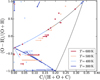 |
Fig. 3 All atmospheres calculated in the parameter space. Some atmospheric compositions change with height due to condensation, leading to tracks. The surface level for each atmospheric track is marked with a star, surface temperature is indicated with colour. |
Number of atmospheres per type and surface temperature.
3.2 Cloud condensates
The removal of thermally stable cloud condensates is an integral part of the models presented here and it allows further constraints to be placed on the surface composition. As the cloud model involved is purely based on the supersaturation ratio and does not include effects such as nucleation and condensation, the approach does not provide an insight to the number of cloud droplets or their size. Therefore, we characterised the different cloud condensates by their abundance relative to the gas phase if a fixed set of element abundances is brought to lower pressures. This led to four different categories of cloud condensates.
Main component condenses: The main species of the gas phase becomes thermally stable as a condensate. Therefore the cloud particle number density relative to the gas phase reaches values of ncond/ngas > 0.5 in the first condensation layer.
Abundant condensates: Cloud particle number density relative to gas phase of ncond/ngas > 10-9.
Trace condensates: Cloud particle number density relative to gas phase of ncond/ngas > 10-12.
Numerical condensates: Within the model, there are further condensates removed from the gas phase. However, these are only present at very low number densities of less than ncond/ngas > 10-12. In this work, we chose not to further investigate such condensates, as their abundances are too low.
The only species that can condense as the main component of the atmosphere is H2O[l], since the main gas species throughout our atmospheric models are: H2O, CO2, CH4, H2, N2, and O2 (see also Table 2). Although CO2 and CH4 have corresponding condensate phases which are included in GGCHEM, they only become thermally stable at temperatures colder than those investigated in this work, leaving H2O as the only dominating atmospheric species to condense. This collapse of the atmosphere appears only in the models with 400 K surface temperature, as they become cold enough for water to condense. We note that such an atmospheric collapse is not seen in any currently known planet.
In the abundant cloud condensates category we find a total of four thermally stable condensates, namely H2O[l,s], C[s], and NH4Cl[s]. Most condensates of this category are found in atmospheres with 300 K, 400 K, and 500K surface temperatures, respectively.
Type B atmospheres with surface temperatures of 300 K and 400 K exclusively condense H2O[l,s]. We find that type A and C atmospheres can contain all of the species in the abundant condensates bin, with NH4Cl[s] only occurring in type A and in atmospheres in the hydrogen-rich portion of type C. At a 500 K surface temperature the only cloud-forming condensate (with ncond/ngas > 10−12) is C[s], found in carbon-rich atmospheres of types A and C. Type B atmospheres remain completely cloud free for Tsurf = 500 K.
The models with 600 K surface temperature give rise to a number of new condensates which are all found in trace abundances. Overall, five different condensates form, which can be sorted into salts (NaCl[s] and KCl[s]), iron sulphides (FeS[s] and FeS2[s]), and metal oxides (Fe2O3[s], Al2O3[s]). Generally we find that C[s] is the only condensate in this temperature regime, which occurs in sufficient amounts which place it in the abundant condensate category. Furthermore C[s] is only found in atmospheres of type A, C, and D. In type D C[s] is the only condensate with ncond/ngas > 10−12. Type B atmospheres only condense NaCl[s] and Al2O3[s] in trace abundance amounts or remain cloud free. In type A we find the condensate species C[s], NaCl[s], and FeS[s]. Furthermore, we note that hydrogenrich type C atmospheric condensates resemble those found in type A. Then, C[s] and NaCl[s] are also found in oxygen-rich type C atmospheres. While FeS[s] is no longer found, additional thermally stable cloud condensates of KCl[s], FeS2[s], and Fe2O3[s] emerge. Notably, Al2O3[s] exclusively occurs in type B atmospheres.
We define an atmosphere as cloud-free if there are no thermally stable condensates with a number density of ncond/ngas > 10−12 . Cloud-free atmospheres exist for every surface temperature with no apparent correlation with atmospheric type. We find that ~33% of atmospheres with Tsurf = 300 K, ~42.9% of atmospheres with Tsurf = 400 K, ~61.9% of atmospheres with Tsurf = 500 K, and ~23.8% of atmospheres with Tsurf = 600 K are cloud-free. However, 3D effects such as temperature difference in the day and night side, which are not considered in this work, could introduce further cloud condensation.
Atmospheres for which one molecule exceeds a mixing ratio of 90%, sorted by the remaining cumulative mixing ratio.
3.3 Atmosphere as an indicator for the crust composition
One main aspect of this study is the investigation of the connection between the atmospheric and crustal composition. Although the crustal composition for each atmosphere is diverse and a total of 83 different condensates are present throughout the investigated parameter space, the presence of some condensates can be linked to the atmospheric composition. The condensates with the strongest links can be separated into five distinctive groups of condensates, which are:
- (a)
Sulphur-bearing species (FeS[s], FeS2[s], CaSO4[s]),
- (b)
Iron oxides (evolution of redox state),
- (c)
Feldspar(KAlSi3O8[s], CaAl2Si2O8[s], NaAlSi3O8[s]),
- (d)
Silicates and silica (Mg2SiO4[s], MgSiO3[s], SiO2[s]), and
- (e)
Carbon compounds (C[s], carbonates).
In the following sections, these different groups are individually discussed in further detail.
3.3.1 Sulphur-bearing species
All models contain the sulphur-bearing species FeS[s] (iron sulfide), FeS2[s] (iron disulfide), and CaSO4[s] (calcium sulfate) in one of four unique combinations; namely, (1) FeS[s]-only, (2) FeS2[s]-only, (3) FeS2[s] coexisting with CaSO4[s], and (4) CaSO4[s]-only.
At Tsurf = 300 K, all but one crust of type A atmospheres have FeS[s]-only. The one exception is the model BSE15, with an oxygen-rich atmosphere at the border from type A to type C, which has FeS2[s]-only instead. Hydrogen-rich type C atmospheres, with more CH4 than CO2, show the presence of FeS2[s] only. Crusts of oxygen-rich type C atmospheres with more CO2 than CH4, have a combination of FeS2[s] and CaSO4[s], with the exception of the VNS model, which exclusively contains FeS2[s] in its crust. All type B atmospheres crusts contain CaSO4[s]-only. The distribution of these different sulphur containing condensates is visualised in the CHO parameter space in Fig. 4.
At Tsurf = 400 K, the link between the sulphur compounds in the crust and the atmospheric type remains largely unchanged from the 300 K case. The only difference is the transition from FeS[s] to FeS2[s], which no longer coincides with the type A-C border, but, rather, it shifts towards lower hydrogen abundances and deeper into the type C atmosphere regime.
At Tsurf = 500 K the trend continues and the transition from FeS[s] to FeS2[s] keeps moving towards lower hydrogen abundances. All crusts of type A and type C atmospheres with CH4≥CO2 content have FeS[s] as the sole sulphur-bearing condensate in their respective crust. In crusts of type C atmospheres where CO2≥CH4, we find three FeS2[s] crusts, one FeS[s] and the remaining are of the mixed FeS2 [s] and CaSO4[s] combination. Type B atmospheres crusts behave like before, containing exclusively CaSO4[s].
For the highest surface temperature investigated in this work (Tsurf = 600 K), crusts with FeS2[s] as the only sulphur-bearing condensate in the crust do not occur. Crusts in contact with type A and C atmospheres generally only contain FeS[s], whereas crust of type B atmospheres contain CaSO4[s] as the exclusive sulphur-bearing species. In the transition region between type B and C atmospheres, the coexistence of FeS2[s] with CaSO4[s] can occur, this is also shown in Fig. 4.
In general, the transition of the sulphur-bearing species in the crust in contact with an atmospheric composition ranging from an overall reduced (hydrogen-rich) to an oxidised (oxygen-rich) atmosphere follows the transition path as
![Mathematical equation: \ce{FeS}[\mathrm{s}] \longleftrightarrow \ce{FeS2}[\mathrm{s}] \longleftrightarrow \left(\ce{FeS2}[\mathrm{s}] + \ce{CaSO4}[\mathrm{s}]\right) \longleftrightarrow \ce{CaSO4}[\mathrm{s}].](/articles/aa/full_html/2025/07/aa53069-24/aa53069-24-eq7.png) (7)
(7)
For higher surface temperatures, the intermediate step of the sole of FeS2 is missing, with the transitions following
![Mathematical equation: \ce{FeS}[\mathrm{s}] \longleftrightarrow \left(\ce{FeS2}[\mathrm{s}] + \ce{CaSO4}[\mathrm{s}]\right) \longleftrightarrow \ce{CaSO4}[\mathrm{s}].](/articles/aa/full_html/2025/07/aa53069-24/aa53069-24-eq8.png) (8)
(8)
This behaviour is shown in Fig. 4. Throughout all temperatures, the crusts in contact with type B atmospheres contain CaSO4[s], with only one model showing the additional presence of FeS2[s].
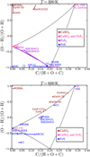 |
Fig. 4 Sulphur-bearing species in crusts at different temperatures, illustrating the transition in sulphur compounds throughout the phase space and surface temperature. The upper and lower panels are calculated for Tsurf = 300K and Tsurf = 600 K, respectively. |
3.3.2 Iron oxides and hydroxides (evolution of redox state)
The crust compositions investigated in this work show the presence of various different iron containing oxides, namely, FeO[s] (Fe(II)oxide), Fe2O3[s] (Fe(III) oxide), FeO2H[s] (Fe(III)oxide-hydroxide), and Fe3O4[s] (Fe(II)(III)oxide). The crusts have either one of these compounds by itself, or the combination of FeO2H[s] and Fe2O3[s], which are both Fe(III) compounds. For some crust compositions, none of these abundant iron-bearing compounds are thermally stable. Such a crust composition will be referred to as none (i.e. no pure iron oxide or hydroxide). However, there are a large number of additional Fe-bearing condensates that are thermally stable. These include Fe2SiO4[s] (fayalite), NaFeSi2O6[s] (aegirine), FeAl2O4[s] (hercynite), Ca3Fe2Si3O12[s] (andradite), FeTiO3[s] (ilmenite), Fe[s] (iron), FeS[s] (ferrous sulfide), FeS2 [s] (iron disulfide), FeAl2SiO7H2[s] (Fe-chloritoid), KFe3AlSi3O12H2[s] (annite), Fe3Si2O9H4[s] (greenalite), Ca2FeAl2Si3O13H[s] (epidote), and FeCO3[s] (siderite).
At Tsurf = 300K and 400 K, all crusts of type A atmospheres as well as atmospheres of type C with CH4>CO2 have either none of the compounds or Fe3O4[s] (Fe(II)(III)) in their crusts. Crusts in contact with type C atmospheres containing CH4<CO2, contain Fe(III) compounds, with one exception (venusNoSurf, None). In crusts with type B atmospheres, Fe2O3[s] (Fe(III)), FeO2H[s] (Fe(III), or both are found.
At 500 K, the behaviour changes slightly for crusts in contact with type C atmospheres. Oxygen-rich atmospheres in type C, which are close to the type B-C border, only contain Fe2O3[s] (Fe(III)). Crusts in contact with hydrogen-rich type C or type A atmospheres, exclusively hold Fe3O4[s] (Fe(II)(III) compound).
At 600 K crusts with type B and C atmospheres are the same as in crusts with cooler surface temperatures. Type A atmospheres crusts contain either none of these compounds, or FeO[s] (Fe(II)).
Overall, crusts in contact with type B atmospheres hold only Fe(III) compounds across all temperatures. Crusts of oxygenrich type C atmospheres behave identical to crusts in contact with type B atmosphere. The rest of the phase space is more ambiguous with crusts containing either none of the mentioned compounds or a mixture of Fe(II) and Fe(III) compounds.
3.3.3 Feldspar diversity
Another group of crust condensates demonstrating some link to the atmospheric type is the feldspar group: KAlSi3O8[s] (orthoclase), CaAl2Si2O8[s] (anorthite), and NaAlSi3O8[s] (albite). With our model, we do not investigate solid solutions of different condensates. Although, in reality, such solid solutions are important, we investigate the presence and co-existence of the different endmembers. While for all surface temperatures models without the thermal stability of any feldspar exist, the following combinations of feldspars are valid for the corresponding surface temperatures:
300 K: KAlSi3O8[s] and NaAlSi3O8[s] individually or together; 400 K: NaAlSi3O8[s] individually or together with KAlSi3O8[s] and/or CaAl2Si2O8[s];
500 K: NaAlSi3O8[s]-only, CaAl2Si2O8[s] combined with NaAlSi3O8[s], and all three;
600 K: none, CaAl2Si2O8[s]-only, CaAl2Si2O8[s] combined with NaAlSi3O8[s], and all three.
We note that the only possible combination of two feldspar endmembers, which we do not find to be thermally stable together in any of our models is KAlSi3O8[s] with CaAl2Si2O8[s].
At 300 K surface temperature, crusts with type A atmospheres are void of any feldspar, with the exception of the MORB model, which contains KAlSi3O8[s] combined with NaAlSi3O8[s]. Close to the type A-C border, in hydrogen-rich type C atmospheres crusts, we find a mixture of different feldspar content in crusts with no apparent correlations. In the remaining parameter space where CH4<CO2 in the crusts of atmospheres in type B and type C, we find KAlSi3O8[s] combined with NaAlSi3O8[s], with the exception of the venus2 model crust with NaAlSi3O8[s] as the only feldspar compound.
At 400 K surface temperature, crusts in contact with type A atmospheres are without feldspar. The only exception is the BSE model with NaAlSi3O8[s] in the crust. In type C atmospheres where CH4≥CO2, the respective crusts are also mostly without feldspar, except for the MORB model, conversely containing all three feldspar compounds. All other models with atmospheres of type C and B, have at least two feldspar species in their respective crusts. Most have KAlSi3O8[s] combined with NaAlSi3O8[s], one CaAl2Si2O8[s] combined with NaAlSi3O8[s] (venus2, type C atmosphere), and two oxygen rich models with all three feldspar species (venusSurf, type C atmosphere and MORBo type B atmosphere).
For 500 K surface temperature, types A and C have no feldspar, with one exception (BSE, type A atmosphere, NaAlSi3O8[s]). The transition to feldspar-bearing crusts happens at higher oxygen abundances than at colder temperatures, at around equal abundance of H and O. More oxygen-rich atmospheres, both in type B and C atmospheres crusts host all three feldspar species, with one exception (venus2, type C atmosphere), with CaAl2Si2O8[s] and NaAlSi3O8[s].
At 600 K the situation changes drastically, with all but two modelled (CI, type A atmosphere and CC type C atmosphere) crusts containing at least one feldspar species. The majority behaves as follows: crusts of atmospheres in type A have CaAl2Si2O8[s]-only, crusts of type B have all three feldspar species, and type C is a mixture of both cases. Three (archean5C, BSE20HCO, BSE30HCO) crusts in type C atmospheres have CaAl2Si2O8-only, one (BSE) has CaAl2Si2O8[s] and NaAlSi3O8[s] combined, the rest of the models has all three feldspar species combined. Those with all three species in type C are the very oxygen-richest of type C, and seem to resemble crusts of type B atmospheres.
Overall, feldspar containing crusts increase with oxygen content in the respective model and with surface temperature. Type B atmospheres crusts consistently have the highest number of unique feldspar species. The question of which species they are depends on the temperature. At high temperatures (600 K), we find feldspar species occur in almost every model, no matter what type the corresponding atmosphere is.
In the cases where a given feldspar endmember is not thermally stable, other condensate species are incorporating the K, Na, and Ca. For K this link between the feldspar and the replacing condensate is the strongest, with KMg3AlSi3O12H2[s] (phlogopite) taking its place. Additionally, KCl[s] (potassium chloride) or K2SiO3 [s] (potassium silicate) occur. Similarly, instead of the thermal stability of the Na-feldspar, NaMg3AlSi3O12H2[s] (sodaphlogopite) can be themally stable. However, there are also further species including Na2SiO3[s] (sodium metasilicate), NaF[s] (sodium fluoride), NaFeSi2O6[s] (acmite), and NaCrSi2O6[s] (kosmochlor) that are thermally stable instead of the Na forms of feldspar and phlogopite. For the Ca-feldspar, the link to the thermal stability of another Ca-bearing condensate is less clear and is depending on the elemental composition and temperature. For crusts in contact with H-rich atmospheres, this does especially include CaMgSi2O6[s] (diopside). For all others, various hydrated minerals and Ca5P3O12F[s] (fluorapatite) are thermally stable instead of the Ca-feldspar.
3.3.4 Silicates and silica
The main silicates found in the crustal compositions in our models are Mg2SiO4[s] (forsterite), MgSiO3 [s] (enstatite), and SiO2[s] (silica). These are found in different combinations of (1) Mg2SiO4[s]-only, (2) Mg2SiO4[s] plus MgSiO3[s], (3) MgSiO3[s]-only, (4) MgSiO3[s] plus SiO2[s], and (5) SiO2[s]-only.
At low surface temperatures (300 and 400 K) the present forms of the crust silicates contents undergo a transition from hydrogen-rich to oxygen-rich atmospheres (type A-C-B) via
![Mathematical equation: \ce{Mg2SiO4}[\mathrm{s}] \longleftrightarrow \mathrm{None} \longleftrightarrow \ce{MgSiO3}[\mathrm{s}] \longleftrightarrow \ce{SiO2}[\mathrm{s}].](/articles/aa/full_html/2025/07/aa53069-24/aa53069-24-eq9.png) (9)
(9)
Two type A models (BSE, MORB), one type C (venusSurf), and one type B (MORBo) are outliers. The MORB, venusSurf, and MORBo models crusts contain MgSiO3[s] plus SiO2[s]. The BSE models crust contains Mg2SiO4[s] with MgSiO3[s]. At 400 K all models still contain the same silicate combination in their crusts as in the 300 K case. Notably, type B atmospheres crusts always contain SiO2 [s] as the only crust silicate and once in combination with MgSiO3[s]. Oxygen rich type C atmospheres crusts, close neighbours to type B, tend to also contain SiO2[s] alone or in combination with MgSiO3[s]. Two models which do not follow that trend are the venus2 model (containing only MgSiO3[s]) and the venus10 model (containing none of the investigated silicates).
At 500 K the transition changes compared to the lower surface temperatures cases. The hydrogen rich part of the phase space (where atmospheres contain CH4≥CO2), respective crusts hold Mg2SiO4[s], with two exceptions, namely the venus10 models crust containing none of the aforementioned compounds and the BSE models crust containing Mg2SiO4[s] plus MgSiO3[s]. Type B and type C oxygen-rich atmospheres crusts behave the same as described in the low temperature regime.
At 600 K the large majority of crusts contain two silicate species. There are three models with crusts that contain only one compound: CI (type A, Mg2SiO4[s]), CC (type C, Mg2SiO4 [s]), and venusNoSurf (type D, MgSiO3). The rest follows a transition from the hydrogen-rich to oxygen-rich part of the parameter space:
![Mathematical equation: \left(\ce{Mg2SiO4}[\mathrm{s}] + \ce{MgSiO3}[\mathrm{s}] \right)\longleftrightarrow \left(\ce{SiO2}[\mathrm{s}] + \ce{MgSiO3}[\mathrm{s}]\right).](/articles/aa/full_html/2025/07/aa53069-24/aa53069-24-eq10.png) (10)
(10)
The transition seems to happen right at the type C-B border, with oxygen-rich type C atmospheres crusts close to the border taking on the in type B atmospheres crusts prevalent SiO2[s] combined with MgSiO3[s] crust silicate combination.
In summary, crusts in contact type B atmospheres always have SiO2[s], either exclusively or in combination with MgSiO3[s] across all examined temperatures. Close to the border between type B and C, oxygen-rich type C atmospheres crusts tend to have the type B atmospheres crusts-typical silicates in their crusts. The rest of the parameter space evolves with surface temperature, from none of the listed silicates at low temperatures to a composition of Mg2SiO4[s]-only and Mg2SiO4[s] combined with MgSiO3[s] at higher temperatures.
3.3.5 Carbon-bearing species
Pure carbon in the crust can only be found in type A and C atmospheres. The elemental carbon content of the atmosphere is then directly given by the supersaturation of C[s]. In accordance with this, no atmospheres exist in the region of CO dominated atmospheres (type D). However, there is one exception (Venus-NoSurf, 600 K), which shows CO>H2O and therefore falls into type D with higher C abundances. With the cooling along the (p, T)-profile, C[s] is removed as a condensate and the atmosphere becomes type C.
Carbonates we find to be thermally stable in our models include CaCO3[s] (calcium carbonate), H2CO3[s] (carbonic acid), MgCO3[s] (magnesium carbonate), MnCO3[s] (manganese carbonate), FeCO3[s] (ferrous carbonate), and NaAlCO5H2[s] (dawsonite). Crust carbonates predominantly occur in low type C atmospheres crusts with Tsurf ≤ 400 K.
At 300 K, there are seven crusts with carbonate compounds, of which four are hydrogen-rich type C atmospheres crusts. These four models are: archean5C and venus10 with CaCO3[s] and MnCO3[s], BSE20HCO with MnCO3[s] and FeCO3[s], and BSE30HCO with MnCO3[s], FeCO3[s], and MgCO3[s]. In addition, there are: one oxygen-rich type C model with the same carbon condensates as BSE30HCO, one type A atmospheres crust with CaCO3[s], and one type B atmospheres crust with NaAlCO5H2[s].
At 400 K, the situation is similar with the majority of crust carbonates occurring in low type C models. In total, six crusts contain carbonates, three are hydrogen-rich type C atmospheres crusts. The three are: BSE20HCO and BSE30HCO, both containing MnCO3[s], FeCO3 [s] and MgCO3[s] in their respective crusts and archean5C with CaCO3[s] in the crust. Similar to the 300K case, we observe one oxygen-rich type C model with the same carbon condensate as BSE20HCO and BSE30HCO, one type A atmospheres crust with CaCO3[s], and one type B atmospheres crust with CaCO3[s]. For higher crust temperatures, crust carbonates seemingly cease to exist with only one model (CC, low type C, CaCO3[s]) at 500 K and one model (CC, high type C, CaCO3[s]) at 600 K.
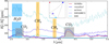 |
Fig. 5 Comparison of transit spectra for three atmospheric types. Type A atmospheres spectra stand out with high transit depth, CH4 features at 3.3 μm, and lack of CO2 features. Spectra originating from atmospheres of type B lack CH4 features. Spectra obtained from type C can (if they display oxygen-rich features) resemble type B spectra or resemble type A spectra if they are hydrogen-rich and show CH4 features. |
3.3.6 Further condensates
Furthermore, a total of 63 additional condensates are found to be thermally stable throughout the investigated parameter space. These include (among others) hydrogen-bearing condensates (phyllosilicates and liquid water), salts, and phosphor compounds.
Water. The formation of phyllosilicates (hydrated minerals) is of vital importance for the presence of water as a long time thermally stable condensate. Such minerals are often thermally favourable to liquid water (e.g. Herbort et al. 2020). These can form over geological times (see Mars Poulet et al. 2005), but also already during the grain formation in the protoplanetary disk (e.g. Thi et al. 2020). Our models show the presence of phyllosilicates in all atmospheric types. Naturally, due to the incorporation of OH groups, phyllosiciates are more frequent and diverse in type A and hydrogen-rich type C atmospheres. We show the possibility that crusts in every atmospheric type can show the stability of water as a crust condensate. We note that independent on the presence of liquid water as a condensate as part of the crust composition and the atmospheric type, water as a cloud species can be present. Therefore simply water vapour or even clouds are not necessarily an indicator for surface water.
Salts. Throughout the models investigated in this work, salts are an omnipresent part of the crust composition. They include sodium chloride NaCl[s] (sodium chloride), KCl[s] (potassium chloride), MgF2[s] (magnesium flouride), CaF2[s] (calcium flouride), NaF[s] (sodium flouride), NH4Cl[s] (ammonium chloride), and AlF6Na3[s] (trisodium hexafluoroaluminate). We note that NaCl[s] occurs in almost every crust, with only one exception (CC, type A, KCl[s] instead) at 300K surface temperature, and at 400 K with only two exceptions (CC, type A, KCl[s] and venus10, type C, forms none of the compounds). For crusts with Tsurf > 500 K less salts are formed in contact with type A atmospheres and hydrogen-rich type C, while crusts of oxygen-rich type C atmospheres and type B atmospheres contain NaCl[s] in combination with MgF2[s].
Phosphorus. One element of limiting importance for the formation of life is phosphorus. As also seen in Herbort et al. (2024), all phosphorus is kept in the crust condensates in the form of hydroxy- and fluorapatite (Ca5P3O13H[s] and Ca5P3O12F[s]). This is independent of the type of the connected atmosphere. Finally, Ca5P3O12F[s] is the principle molecule and Ca5P3O13H[s] only occurs alongside it.
3.4 Theoretical transmission spectra
In Section 3.3, we investigate the link between certain crust forming condensates and the atmospheric types defined by atmospheric composition. In this section, we investigate how far the different atmospheric types can be differentiated with transmission spectroscopy. Overall, the main contribution to the spectra are provided by the main gas phase components of CO2, CH4, NH3, and H2O. Other species, especially H2, have a significant impact on the mean molecular weight and thus on the feature depth. Different spectra with some marked features can be seen in Fig. 5.
In general, atmospheres of type A can be identified with a spectra by (1) their lack of strong CO2 features at Tsurf ≤ 400 K, (2) CH4 features, (3) a prominent double NH3 feature at around 11 μm, and (4) often low mean molecular weight due to higher hydrogen content resulting in inflated atmospheres and larger than usual transit depths. The fourth criterion becomes less of a distinguishing factor with higher temperatures. This is caused by the fact that atmospheres (with or without an abundance of hydrogen) show larger absorption depth with increased temperature due to the larger scale height. The largest differences in transit depth due to low mean molecular weight in type A atmospheres spectra are around 100 ppm for the lowest Tsurf of 300 K. For higher Tsurf the peak to valley difference shrinks to about 50 ppm. For Tsurf ≥ 500 K CO2 features start to appear in the spectrum, making the differentiation between type A and C atmospheres more difficult. This degeneracy can be solved by a NH3 feature at around 11 μm, which does not appear in spectra originating from type C atmospheres.
The spectra of atmospheres in type B show signals of (1) strong CO2 features, (2) H2O features in all spectra with Tsurf ≥ 400 K, and (3) lack of CH4 features. Due to their small transit depths, spectra of type B atmospheres are the most difficult to observe. The strongest features (CO2, H2O) are ~10 ppm strong at 300 K, while they roughly double for hotter Tsurf.
Type C atmospheric spectra are more ambiguous. Hydrogenrich type C atmospheres tend to take on traits from type A atmospheres spectra; for instance, CH4 features. In that case, they are still possible to tell apart from typical type A atmospheres spectra via CO2 features for cool surface temperatures below 500 K (Fig. 6). As mentioned above, type A atmospheres spectra can display CO2 features for higher temperatures which would make distinguishing between the two types from spectra alone impossible. However, spectra from type C atmospheres never show NH3 features, which are exclusive to type A (Fig. 7). Oxygen-rich type C atmospheres spectra behave entirely different. These spectra can be void of any CH4 features and can mimic type B atmospheres spectral features with no distinguishable qualities, despite originating from type C atmospheres. Only the very oxygen-richest type C atmospheres spectra are affected by this, as shown in Fig. 8. When oxygen becomes less abundant CH4 features arise quickly.
The only spectrum of a type D atmosphere resembles those of type C atmospheres. As the type D is only found in the near-crust atmosphere and due to the removal of C as C[s], the atmosphere transitions to an oxygen-rich type C.
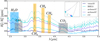 |
Fig. 6 Comparison between spectra from type A and C atmospheres. All spectra have a sharp CH4 feature at 3.3 μm. Spectra originating from atmospheres of type C show a defined CO2 feature at around 4.3 μm, which can be used to differentiate between the two types. However, in the CC (type A) model, a soft CO2 feature emerges at 4.3 μm. |
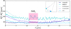 |
Fig. 7 Comparison between spectra from type A and C atmospheres. When CO2 start to emerge in type A atmospheres at higher surface temperatures, the spectra resemble those of type C atmospheres. It is, however, possible to use a NH3 feature in type A atmospheres spectra, to retrieve the atmospheric type from spectra alone. |
3.5 Graphite stability
We observe that the condensation of C[s] as a thermally stable cloud condensate is not only unique because it can occur for any surface temperature, but it is also the only thermally stable condensate in the isothermal part of the atmospheric profile. Here, the removal of purely carbon also has the effect that the atmospheric type can change from type C to type A atmospheres. The nature of this behaviour at low pressures and low partial pressures of carbon (i.e. high abundances of nitrogen) is visualised in Fig. 9. Here, the contour lines of the supersaturation of C[s] of unity are indicated for different nitrogen abundances throughout the CHO-parameter space.
4 Summary
In this paper, we model planetary surfaces and atmospheres, together in a linked bottom-to-top model. The crust-atmosphere interaction layer is in chemical and phase equilibrium. Throughout the atmosphere, a parcel of air follows a simple (p, T)-structure and the chemical and phase equilibrium is solved. Any thermally stable condensate throughout the atmosphere is removed as a cloud condensate and depletes the affected elements in the atmosphere above. Our models have been tested for Earth-sized planets with four different surface temperatures. Based on these atmospheric compositions, transmission spectra are calculated with the planets orbiting an M1 type star at distances corresponding to their surface temperature. This approach allows us to investigate the link between the observables and surface compositions for a diverse set of surface and atmospheric compositions.
We explored links between atmospheric type and crust composition. Although the link is in general ambiguous and nonunique, it is possible to define groups of stable crust condensates which exhibit links between the corresponding atmospheres type and crust composition. In particular, for crusts that are in contact with the oxygen-rich atmospheric type B, they stand out due to their sharply defined boundaries for respective crust compositions across all surface temperatures. The composition of crusts in contact with atmospheres of the other types (A, C, and D) show a temperature-dependent behaviour, with boundaries between certain crust compositions evolving with surface temperature, at times not adhering to atmospheric type borders.
Crust sulphur, occurring in the forms of FeS[s], FeS2[s], and CaSO4[s], is tightly linked to the contacting atmosphere. We find that crusts of type B atmospheres always contain CaSO4[s] and only rarely in combination with FeS2[s]. In contrast, no type A or D atmospheres crust contains CaSO4[s] alone, these crusts contain FeS[s] or FeS2[s]. Crusts in contact with type C atmospheres can display either of the compound combinations, depending on oxygen and hydrogen content and temperature. Sulphur chemistry in general seems to be a promising candidate for atmosphere crust links. H2SO4[l,s] cloud condensates indicate high surface pressure and temperatures (Herbort et al. 2022) and are incompatible with liquid water as a surface condensate (Loftus et al. 2019; Jordan et al. 2025).
Iron oxides and hydroxides show a similar behaviour, with more oxygen-rich models also containing iron in a more oxidised state. Crusts with type B atmospheres bear iron(III) compounds, while crusts in contact with type A and C atmospheres tend to contain the less oxidised iron(II) or iron(II)(III) compounds. Showing a range of different oxidisation states expected for different planetary atmospheres (Guimond et al. 2023; Nicholls et al. 2024). Furthermore, it should be noted that the oxidisation state of the condensates for a constant O/H can drastically differ.
For the further condensates, we find that silica (SiO2[s]) and the silicate species Mg2SiO4[s] and MgSiO3[s] show links to the corresponding atmospheric type. The number of species present increases with temperature. The number of feldspar endmembers is generally increasing with higher oxygen abundances (type B, type C with CH4<CO2). Although these trends are presented in the models here, we note that further geological processes are likely to play a role. For example, the different feldspars are present in a solid solution instead of the pure endmember states, especially at or quenched at high temperatures (see e.g. Wood & Nicholls 1978; Klein & Philpotts 2013, for further reading). Furthermore, active geological processes can reshape the mineral composition in the planetary interior. GGCHEM does not include solid solutions, instead geological models such as PERPLE_X (Myhill & Connolly 2021) can be used to follow up on the presence of different minerals in the planetary surface compositions.
Pure C[s] is only found in crusts of type A and C atmospheres and can be linked to carbon clouds in the atmosphere. Carbonates predominantly form in crusts with low surface temperatures (300 K and 400 K) in crusts in contact with type C atmospheres. While for type-C atmospheres, C[s] becomes thermally table in the lower parts of the atmosphere, for type A atmospheres, it is possible to have low-pressure thermal stability of C[s]. This low-pressure regime coincides with an almost isothermal (p, T)-profile, which is unlikely to be present in the upper atmosphere due to stellar heating (see also e.g. Van Looveren et al. 2025). An increasing temperature will reduce the supersaturation ratio for any condensible species.
Further crust condensates show either weak or no links with the respective atmosphere above. Phyllosilicates are more frequent at low temperatures, salts are most numerous at low surface temperatures and oxygen-rich atmospheres crusts, phosphor compounds show no correlation with atmospheric type, manganese(III)-oxide is most frequent in the oxygen-rich type B atmospheres crusts, and Ca-Ti-Al compounds show a weak link between the atmosphere and the surface.
Observing these atmospheres with transmission spectroscopy allows us, in principle, to distinguish between the atmospheric types and therefore to constrain the surface minerals. The spectra of type A atmospheres can be characterised by (1) low mean molecular weight, (2) strong CH4 absorption features, (3) the existence of NH3 features, and (4) the lack of strong CO2 features at low surface temperatures. Spectra originating from type B atmospheres are defined by (1) strong CO2 features, (2) H2O features for warm surface temperatures, and (3) lack of CH4 absorption features. The spectra of hydrogenrich Type C atmospheres mimic those of type A atmospheres, but can be distinguished by the lack of NH3 absorption features. While moderately oxygen-rich type C atmospheres are distinct from spectra for type B atmospheres, the spectra for the most oxygen-rich type C atmospheres seem to be indistinguishable from those for carbon-rich type B atmospheres.
Throughout this work, we have investigated atmospheric models, which include the effect of element depletion due to cloud condensation. The effect of clouds on the spectra itself has been omitted, as this is a more diverse influence based (among other aspects) on the cloud condensate density, composition, and size distribution. Furthermore, planets are inherently threedimensional objects, which causes differences in the morning and evening terminator as they are probed simultaneously during transmission spectroscopy. This effect is stronger for more pronounced day-to-night-side differences. See e.g. Helling et al. (2023) for gas giants or Nguyen et al. (2024) for magma ocean planets. Therefore, the transmission spectra presented here must be seen as an theoretical idealised scenario. While the precision needed to distinguish among the different spectra presented here is challenging for instruments on JWST, future missions such as HWO and LIFE might be able to shed light on these differences.
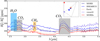 |
Fig. 8 Displaying the sudden change in spectral features for oxygen-rich atmospheric spectra. Type B atmospheres spectra do not show any CH4 features, as do type C, which are extremely oxygen-rich. Both show similar spectra, with CO2 features. In spectra from hydrogen rich, ‘deeper’ type C atmospheres, strong CH4 feature appear. |
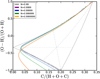 |
Fig. 9 Influence of the nitrogen elemental abundance on the C[s] supersaturation ratio. The different lines indicate the graphite supersaturation ratio of unity for different abundances of nitrogen. The pressure is fixed for all models to 10−5 bar. |
Acknowledgements
The authors thank R.J. Spaargaren for his valuable discussions on (exoplanet) mineralogy.
Appendix A Supplementary material
Elemental mass frthtions of the sets of element abundances used in this work.
All thermally stable condensates throughout this work with their name, chemical, and sum formula, and whether they are present as cloud and/or crust condensates.
References
- Ackerman, A. S., & Marley, M. S. 2001, ApJ, 556, 872 [Google Scholar]
- Alei, E., Quanz, S. P., Konrad, B. S., et al. 2024, A&A, 689, A245 [NASA ADS] [CrossRef] [EDP Sciences] [Google Scholar]
- Arevalo, Ricardo, J., & McDonough, W. F. 2010, Chem. Geol., 271, 70 [NASA ADS] [CrossRef] [Google Scholar]
- Asensio Ramos, A., & Pallé, E. 2021, A&A, 646, A4 [NASA ADS] [CrossRef] [EDP Sciences] [Google Scholar]
- Baumeister, P., & Tosi, N. 2023, A&A, 676, A106 [NASA ADS] [CrossRef] [EDP Sciences] [Google Scholar]
- Baumeister, P., Tosi, N., Brachmann, C., Grenfell, J. L., & Noack, L. 2023, A&A, 675, A122 [NASA ADS] [CrossRef] [EDP Sciences] [Google Scholar]
- Byrne, X., Shorttle, O., Jordan, S., & Rimmer, P. B. 2024, MNRAS, 527, 10748 [Google Scholar]
- Gaillard, F., Bouhifd, M. A., Füri, E., et al. 2021, Space Sci. Rev., 217, 22 [NASA ADS] [CrossRef] [Google Scholar]
- Gaillard, F., Bernadou, F., Roskosz, M., et al. 2022, Earth Planet. Sci. Lett., 577, 117255 [CrossRef] [Google Scholar]
- Gardner, J. P., Mather, J. C., Abbott, R., et al. 2023, PASP, 135, 068001 [NASA ADS] [CrossRef] [Google Scholar]
- Gilmozzi, R., & Spyromilio, J. 2007, The Messenger, 127, 3 [NASA ADS] [Google Scholar]
- Greene, T. P., Bell, T. J., Ducrot, E., et al. 2023, Nature, 618, 39 [NASA ADS] [CrossRef] [Google Scholar]
- Grenfell, J. L., Leconte, J., Forget, F., et al. 2020, Space Sci. Rev., 216, 98 [CrossRef] [Google Scholar]
- Guimond, C. M., Noack, L., Ortenzi, G., & Sohl, F. 2021, Phys. Earth Planet. Interiors, 320, 106788 [CrossRef] [Google Scholar]
- Guimond, C. M., Shorttle, O., Jordan, S., & Rudge, J. F. 2023, MNRAS, 525, 3703 [NASA ADS] [CrossRef] [Google Scholar]
- Guimond, C. M., Wang, H., Seidler, F., et al. 2024, Rev. Mineral. Geochem., 90, 259 [Google Scholar]
- Hammond, M., Guimond, C. M., Lichtenberg, T., et al. 2025, ApJ, 978, L40 [Google Scholar]
- Helling, C. 2022, arXiv e-prints [arXiv:2205.00454] [Google Scholar]
- Helling, C., Samra, D., Lewis, D., et al. 2023, A&A, 671, A122 [NASA ADS] [CrossRef] [EDP Sciences] [Google Scholar]
- Herbort, O., Woitke, P., Helling, C., & Zerkle, A. 2020, A&A, 636, A71 [EDP Sciences] [Google Scholar]
- Herbort, O., Woitke, P., Helling, C., & Zerkle, A. L. 2022, A&A, 658, A180 [NASA ADS] [CrossRef] [EDP Sciences] [Google Scholar]
- Herbort, O., Woitke, P., Helling, C., & Zerkle, A. L. 2024, Int. J. Astrobiol., 23, 12 [Google Scholar]
- Hu, R. 2021, ApJ, 921, 27 [NASA ADS] [CrossRef] [Google Scholar]
- Hu, R., Bello-Arufe, A., Zhang, M., et al. 2024, Nature, 630, 609 [NASA ADS] [CrossRef] [Google Scholar]
- Janson, M., Henning, T., Quanz, S. P., et al. 2022, Exp. Astron., 54, 1223 [Google Scholar]
- Janssen, L. J., Woitke, P., Herbort, O., et al. 2023, Astron. Nachr., 344, e20230075 [NASA ADS] [CrossRef] [Google Scholar]
- Jordan, S., Shorttle, O., & Rimmer, P. B. 2025, Sci. Adv., 11, eadp8105 [Google Scholar]
- Kasting, J. F. 1982, J. Geophys. Res., 87, 3091 [NASA ADS] [CrossRef] [Google Scholar]
- Kimura, T., & Ikoma, M. 2022, Nat. Astron., 6, 1296 [NASA ADS] [CrossRef] [Google Scholar]
- Kite, E. S., & Schaefer, L. 2021, ApJ, 909, L22 [NASA ADS] [CrossRef] [Google Scholar]
- Kite, E. S., Fegley, Bruce, J., Schaefer, L., & Gaidos, E. 2016, ApJ, 828, 80 [NASA ADS] [CrossRef] [Google Scholar]
- Klein, C., & Philpotts, A. 2013, Earth Materials: Introduction to Mineralogy and Petrology, Earth Materials: Introduction to Mineralogy and Petrology (Cambridge University Press) [Google Scholar]
- Kreidberg, L., Bean, J. L., Désert, J.-M., et al. 2014, Nature, 505, 69 [Google Scholar]
- Leconte, J., Wu, H., Menou, K., & Murray, N. 2015, Science, 347, 632 [NASA ADS] [CrossRef] [Google Scholar]
- Lee, E. K. H., Tsai, S.-M., Moses, J. I., et al. 2024, ApJ, 976, 231 [Google Scholar]
- Lichtenberg, T., & Miguel, Y. 2025, Treatise Geochem., 7, 51 [Google Scholar]
- Lichtenberg, T., Schaefer, L. K., Nakajima, M., & Fischer, R. A. 2022, Geophysical Evolution During Rocky Planet Formation [Google Scholar]
- Liggins, P., Jordan, S., Rimmer, P. B., & Shorttle, O. 2023, J. Geophys. Res. (Planets), 128, e2022JE007528 [Google Scholar]
- Lodders, K., & Fegley, B. 2024, arXiv e-prints [arXiv:2410.11138] [Google Scholar]
- Lodders, K., Palme, H., & Gail, H. P. 2009, Landolt Börnstein, 4B, 712 [Google Scholar]
- Loftus, K., Wordsworth, R. D., & Morley, C. V. 2019, ApJ, 887, 231 [NASA ADS] [CrossRef] [Google Scholar]
- Lustig-Yaeger, J., Fu, G., May, E. M., et al. 2023, Nat. Astron., 7, 1317 [NASA ADS] [CrossRef] [Google Scholar]
- Madden, J. H., & Kaltenegger, L. 2018, Astrobiology, 18, 1559 [NASA ADS] [CrossRef] [Google Scholar]
- Mbarek, R., & Kempton, E. M. R. 2016, ApJ, 827, 121 [CrossRef] [Google Scholar]
- Miguel, Y., Kaltenegger, L., Fegley, B., & Schaefer, L. 2011, ApJ, 742, L19 [NASA ADS] [CrossRef] [Google Scholar]
- Min, M., Ormel, C. W., Chubb, K., Helling, C., & Kawashima, Y. 2020, A&A, 642, A28 [NASA ADS] [CrossRef] [EDP Sciences] [Google Scholar]
- Myhill, R., & Connolly, J. A. D. 2021, Contrib. Mineral. Petrol., 176, 86 [Google Scholar]
- National Academies of Sciences, Engineering, and Medicine 2021, Pathways to Discovery in Astronomy and Astrophysics for the 2020s (Washington, DC: The National Academies Press) [Google Scholar]
- Nguyen, T. G., Cowan, N. B., & Dang, L. 2024, AJ, 168, 287 [Google Scholar]
- Nicholls, H., Lichtenberg, T., Bower, D. J., & Pierrehumbert, R. 2024, J. Geophys. Res. (Planets), 129, 2024JE008576 [Google Scholar]
- Noack, L., & Breuer, D. 2014, Planet. Space Sci., 98, 41 [NASA ADS] [CrossRef] [Google Scholar]
- Ortenzi, G., Noack, L., Sohl, F., et al. 2020, Sci. Rep., 10, 10907 [NASA ADS] [CrossRef] [Google Scholar]
- Poulet, F., Bibring, J. P., Mustard, J. F., et al. 2005, Nature, 438, 623 [Google Scholar]
- Quanz, S. P., Absil, O., Benz, W., et al. 2021, Exp. Astron., 54, 1197 [Google Scholar]
- Quanz, S. P., Ottiger, M., Fontanet, E., et al. 2022, A&A, 664, A21 [NASA ADS] [CrossRef] [EDP Sciences] [Google Scholar]
- Rauer, H., Aerts, C., Cabrera, J., et al. 2025, Exp. Astron., 59, 26 [Google Scholar]
- Rimmer, P. B., & Helling, C. 2016, ApJS, 224, 9 [NASA ADS] [CrossRef] [Google Scholar]
- Rimmer, P. B., Jordan, S., Constantinou, T., et al. 2021, Planet. Sci. J., 2, 133 [NASA ADS] [CrossRef] [Google Scholar]
- Rogers, J. G., Dorn, C., Aditya Raj, V., Schlichting, H. E., & Young, E. D. 2025, ApJ, 979, 79 [Google Scholar]
- Rossi, L., & Stam, D. M. 2017, A&A, 607, A57 [NASA ADS] [CrossRef] [EDP Sciences] [Google Scholar]
- Rossi, L., & Stam, D. M. 2018, A&A, 616, A117 [NASA ADS] [CrossRef] [EDP Sciences] [Google Scholar]
- Rossi, L., Berzosa-Molina, J., Desert, J.-M., et al. 2022, Exp. Astron., 54, 1187 [Google Scholar]
- Rugheimer, S., Kaltenegger, L., Segura, A., Linsky, J., & Mohanty, S. 2015, ApJ, 809, 57 [Google Scholar]
- Schaefer, L., Lodders, K., & Fegley, B. 2012, ApJ, 755, 41 [NASA ADS] [CrossRef] [Google Scholar]
- Seidler, F. L., Sossi, P. A., & Grimm, S. L. 2024, A&A, 691, A159 [NASA ADS] [CrossRef] [EDP Sciences] [Google Scholar]
- Spaargaren, R. J., Ballmer, M. D., Bower, D. J., Dorn, C., & Tackley, P. J. 2020, A&A, 643, A44 [NASA ADS] [CrossRef] [EDP Sciences] [Google Scholar]
- Surkov, Y. A., Moskalyova, L. P., Moskaleva, L. P., et al. 1986, J. Geophys. Res., 91, E215 [NASA ADS] [CrossRef] [Google Scholar]
- Thi, W. F., Hocuk, S., Kamp, I., et al. 2020, A&A, 635, A16 [NASA ADS] [CrossRef] [EDP Sciences] [Google Scholar]
- Thompson, M. A., Telus, M., Schaefer, L., et al. 2021, Nat. Astron., 5, 575 [NASA ADS] [CrossRef] [Google Scholar]
- Thompson, M. A., Telus, M., Edwards, G. H., et al. 2023, Planet. Sci. J., 4, 185 [Google Scholar]
- Timmermann, A., Shan, Y., Reiners, A., & Pack, A. 2023, A&A, 676, A52 [NASA ADS] [CrossRef] [EDP Sciences] [Google Scholar]
- Tinetti, G., Drossart, P., Eccleston, P., et al. 2018, Exp. Astron., 46, 135 [NASA ADS] [CrossRef] [Google Scholar]
- Tsai, S.-M., Malik, M., Kitzmann, D., et al. 2021, ApJ, 923, 264 [NASA ADS] [CrossRef] [Google Scholar]
- van Buchem, C. P. A., Miguel, Y., Zilinskas, M., & van Westrenen, W. 2023, Meteor. Planet. Sci., 58, 1149 [NASA ADS] [CrossRef] [Google Scholar]
- Van Looveren, G., Güdel, M., Boro Saikia, S., & Kislyakova, K. 2024, A&A, 683, A153 [Google Scholar]
- Van Looveren, G., Boro Saikia, S., Herbort, O., et al. 2025, A&A, 694, A310 [NASA ADS] [CrossRef] [EDP Sciences] [Google Scholar]
- Woitke, P., Helling, C., Hunter, G., et al. 2018, A&A, 614, A1 [NASA ADS] [CrossRef] [EDP Sciences] [Google Scholar]
- Woitke, P., Herbort, O., Helling, C., et al. 2021, A&A, 646, A43 [NASA ADS] [CrossRef] [EDP Sciences] [Google Scholar]
- Wood, B. J., & Nicholls, J. 1978, Contrib. Mineral. Petrol., 66, 389 [Google Scholar]
- Xue, Q., Bean, J. L., Zhang, M., et al. 2024, ApJ, 973, L8 [NASA ADS] [CrossRef] [Google Scholar]
- Zieba, S., Kreidberg, L., Ducrot, E., et al. 2023, Nature, 620, 746 [NASA ADS] [CrossRef] [Google Scholar]
- Zilinskas, M., Miguel, Y., van Buchem, C. P. A., & Snellen, I. A. G. 2023, A&A, 671, A138 [NASA ADS] [CrossRef] [EDP Sciences] [Google Scholar]
All Tables
Atmospheres for which one molecule exceeds a mixing ratio of 90%, sorted by the remaining cumulative mixing ratio.
All thermally stable condensates throughout this work with their name, chemical, and sum formula, and whether they are present as cloud and/or crust condensates.
All Figures
|
Fig. 1 Comparison of our atmospheric profile model for Tsurf = 300 K, 400 K, 500 K, 600 K, Tmin = 0.75 · Tsurf, and κ = 0.9 in comparison to Earth’s atmospheric profile. |
| In the text | |
|
Fig. 2 Parameter space for CHNO element abundances based on Woitke et al. (2021). Solar System rocky bodies atmospheres are indicated with a star. The different atmospheric types defined by the presence of different molecules (see Eq. (4)) are also indicated. |
| In the text | |
|
Fig. 3 All atmospheres calculated in the parameter space. Some atmospheric compositions change with height due to condensation, leading to tracks. The surface level for each atmospheric track is marked with a star, surface temperature is indicated with colour. |
| In the text | |
|
Fig. 4 Sulphur-bearing species in crusts at different temperatures, illustrating the transition in sulphur compounds throughout the phase space and surface temperature. The upper and lower panels are calculated for Tsurf = 300K and Tsurf = 600 K, respectively. |
| In the text | |
|
Fig. 5 Comparison of transit spectra for three atmospheric types. Type A atmospheres spectra stand out with high transit depth, CH4 features at 3.3 μm, and lack of CO2 features. Spectra originating from atmospheres of type B lack CH4 features. Spectra obtained from type C can (if they display oxygen-rich features) resemble type B spectra or resemble type A spectra if they are hydrogen-rich and show CH4 features. |
| In the text | |
|
Fig. 6 Comparison between spectra from type A and C atmospheres. All spectra have a sharp CH4 feature at 3.3 μm. Spectra originating from atmospheres of type C show a defined CO2 feature at around 4.3 μm, which can be used to differentiate between the two types. However, in the CC (type A) model, a soft CO2 feature emerges at 4.3 μm. |
| In the text | |
|
Fig. 7 Comparison between spectra from type A and C atmospheres. When CO2 start to emerge in type A atmospheres at higher surface temperatures, the spectra resemble those of type C atmospheres. It is, however, possible to use a NH3 feature in type A atmospheres spectra, to retrieve the atmospheric type from spectra alone. |
| In the text | |
|
Fig. 8 Displaying the sudden change in spectral features for oxygen-rich atmospheric spectra. Type B atmospheres spectra do not show any CH4 features, as do type C, which are extremely oxygen-rich. Both show similar spectra, with CO2 features. In spectra from hydrogen rich, ‘deeper’ type C atmospheres, strong CH4 feature appear. |
| In the text | |
|
Fig. 9 Influence of the nitrogen elemental abundance on the C[s] supersaturation ratio. The different lines indicate the graphite supersaturation ratio of unity for different abundances of nitrogen. The pressure is fixed for all models to 10−5 bar. |
| In the text | |
Current usage metrics show cumulative count of Article Views (full-text article views including HTML views, PDF and ePub downloads, according to the available data) and Abstracts Views on Vision4Press platform.
Data correspond to usage on the plateform after 2015. The current usage metrics is available 48-96 hours after online publication and is updated daily on week days.
Initial download of the metrics may take a while.