| Issue |
A&A
Volume 699, July 2025
|
|
|---|---|---|
| Article Number | A193 | |
| Number of page(s) | 12 | |
| Section | Astrophysical processes | |
| DOI | https://doi.org/10.1051/0004-6361/202452668 | |
| Published online | 07 July 2025 | |
Orbit design for mitigating interstellar scattering effects in Earth-space very long baseline interferometry observations of Sagittarius A*
1
Department of Physics, National Institute of Technology Surathkal, Karnataka 575025, India
2
Faculty of Aerospace Engineering, Delft University of Technology, 2629HS Delft, The Netherlands
3
KISPE Limited, Farnborough, United Kingdom
4
Center for Astrophysics | Harvard & Smithsonian, 60 Garden Street, Cambridge, MA 02138, USA
5
Black Hole Initiative at Harvard University, 20 Garden Street, Cambridge, MA 02138, USA
⋆ Corresponding author: This email address is being protected from spambots. You need JavaScript enabled to view it.
Received:
18
October
2024
Accepted:
9
April
2025
Abstract
The black hole Sagittarius A* (Sgr A*) is a prime target for next-generation Earth-space very long baseline interferometry missions such as the Black Hole Explorer (BHEX), which aims to probe baselines on the order of 20 Gλ. At these baselines, Sgr A* observations will be affected by the diffractive scattering effects from the interstellar medium (ISM). Therefore, we study how different parameter choices for turbulence in the ISM affect BHEX’s observational capabilities to probe strong lensing features of Sgr A*. By using a simple geometric model of concentric Gaussian rings for Sgr A*’s photon ring signal and observing at 320 GHz, we find that the BHEX-ALMA baseline has the required sensitivity to observe Sgr A* for a broad range of values of the power-law index of density fluctuations in the ISM and the inner scale of turbulence. For other baselines with moderate sensitivities, a strong need for observations at shorter scales of ≈13.5 Gλ is identified. For this purpose, an orbit migration scheme is proposed. It is modeled using both chemical propulsion (CP)-based Hohmann transfers and electric propulsion (EP)-based orbit raising with the result that a CP-based transfer can be performed in a matter of hours, but with a significantly higher fuel requirement as compared to EP which, however, requires a transfer time of around 6 weeks. The consequences of these orbits for probing Sgr A*’s space-time are studied by quantifying the spatial resolution, temporal resolution, and angular sampling of the photon ring signal in the Fourier coverage of each of these orbits. We show that higher orbits isolate space-time features while sacrificing both signal lost to scattering and temporal resolution, but gaining greater access to the morphology of the photon ring. Thus, we find that orbits between the low Earth regime and the reference BHEX orbit can provide rich access to Sgr A*’s parameter space.
Key words: black hole physics / scattering / techniques: high angular resolution / techniques: interferometric
© The Authors 2025
 Open Access article, published by EDP Sciences, under the terms of the Creative Commons Attribution License (https://creativecommons.org/licenses/by/4.0), which permits unrestricted use, distribution, and reproduction in any medium, provided the original work is properly cited.
This article is published in open access under the Subscribe to Open model. This email address is being protected from spambots. You need JavaScript enabled to view it. to support open access publication.
1. Introduction
The observations by the Event Horizon Telescope (EHT) collaboration have opened a new window for probing the strong gravity regime near black holes. Through the technique of very long baseline interferometry (VLBI) (Thompson et al. 2017), a virtual Earth-sized telescope has produced near-horizon images of the Messier 87* (hereafter M87*) (Event Horizon Telescope Collaboration 2019a,b, 2024b) and Sagittarius A* (hereafter Sgr A*) (Event Horizon Telescope Collaboration 2022a) black holes. These images have improved our understanding of the interplay between lensing and polarization (Event Horizon Telescope Collaboration 2021; Goddi et al. 2021), discriminating magnetic field morphology near black holes (Yuan et al. 2022) and serving as an arbiter of supermassive black hole mass measurements (Event Horizon Telescope Collaboration 2019c). We expect that the results recently reported by the EHT of observing M87* at 345 GHz (Raymond et al. 2024) will continue to stimulate research in these directions.
The EHT collaboration plans to continue observing M87* and Sgr A* with improvements in both software and instrumentation design (The Event Horizon Telescope Collaboration 2024). Ground-based expansions that will increase the number of sites and expand their frequency coverage (Doeleman et al. 2023) are also planned. However, such terrestrial observations are subject to fundamental limitations. In particular, the maximum possible baseline length is restricted by the Earth’s diameter. Therefore, since angular resolution θ is related to the observing wavelength, λ, and distance, d, between stations by the relation θ ≈ λ/d, for a fixed wavelength, longer baselines can only be achieved by adding a space-based orbiter. Indeed, at 320 GHz, assuming Earth’s diameter to be d ≈ 12.756 × 10⁶ m, the maximum length of terrestrial baselines is ≈13.5 Gλ. The subsequent improvement in angular resolution is expected to help probe the black hole’s photon ring (Johnson et al. 2020), a strong lensing feature of optically thin accretion that is largely governed by the properties of the black hole space-time and thereby encodes its mass and spin. However, as shown by Shavelle & Palumbo (2024) and Palumbo et al. (2023, hereafter PWCJ), it is possible that ground-based polarimetric observations can begin to detect the presence of the photon ring, if not measure its morphology.
It is therefore natural that there have been several recent investigations into developing the science case for next-generation black hole imaging missions with a space-based orbiter, building upon lessons from prior space VLBI missions (Gurvits 2020). On the one hand, concepts have been proposed of performing space-space VLBI (Roelofs et al. 2019; Trippe et al. 2023; Hudson et al. 2023; Shlentsova et al. 2024) with two or more orbiters that can offer extremely high angular resolution by forming baselines that are several multiples of those permitted by the Earth’s diameter and can perform observations at much higher frequencies that are also uncorrupted by the effects of the Earth’s atmosphere. On the other hand, there are proposals of performing Earth-space VLBI with one (Likhachev et al. 2022; Johnson et al. 2024) or more (Palumbo et al. 2019; Fish et al. 2020) space orbiters that offer the prospect of having improved angular resolution using long baselines, while also having a dense sampling of the (u, v) coverage through the ground array. Furthermore, several complementary studies have been performed that highlight the utility of orbit design and optimization for performing VLBI observations of M87* and Sgr A* with a space-based component (Fromm et al. 2021; Andrianov et al. 2021; Likhachev et al. 2022; Tamar et al. 2024).
For this paper, the reference specifications are of the Black Hole Explorer (BHEX) mission (Johnson et al. 2024) which aims to place an orbiter in a circular, polar orbit at an altitude of 20 192 km to achieve Earth-space baselines on the order of 20 Gλ. The observations at such long baselines at a frequency of 240–320 GHz in its primary receiver, are crucial for one of its main science goals of observing the photon rings of M87* and Sgr A*. The science goals of the mission, as well as details of BHEX’s proposed payload and spacecraft systems, are given in (Johnson et al. 2024).
There are several astrophysical motivations for performing near-horizon science with Sgr A*. It has the largest “shadow” size (∼50 μas) among all of the black holes observed by the EHT (Event Horizon Telescope Collaboration 2022b). Of particular relevance for BHEX is the fact that since Sgr A*’s mass is well constrained to ∼4.1 million M⊙ (Ghez et al. 2008; GRAVITY Collaboration 2019), probing its photon ring can provide a space-time-driven measurement of the black hole’s spin (Gralla & Lupsasca 2020; Broderick et al. 2022; Cárdenas-Avendaño & Lupsasca 2023). However, its observations are complicated by several factors. In particular, Sgr A* has a distinct, anisotropic diffractive scattering component that diminishes the signal on long baselines (Johnson et al. 2018, hereafter J18). This is tricky for missions such as BHEX whose proposed orbit lies at these baseline lengths (Johnson et al. 2024). We note that the RadioAstron mission has already made space VLBI observations of Sgr A* (Johnson et al. 2021) but crucially no detections were reported on the baselines formed with the Spektr-R orbiter. Moreover, the maximum baseline lengths probed were ≈250 Mλ, which is around two orders of magnitude shorter than the ones accessible to BHEX. Thus, while going to such long baselines may be useful for observing the photon ring of M87* (PWCJ), the Sgr A* signal might actually be dominant on relatively shorter baselines beyond which the signal becomes prohibitively difficult to capture.
An additional concern in studies of the photon ring is the need to capture many realizations of the plasma configuration around the black hole. Sgr A*’s mass, approximately 1500 times smaller than that of M87* (Event Horizon Telescope Collaboration 2022a), sets a shorter dynamical timescale around the black hole, on the order of tens of minutes; for example, the innermost stable circular orbit for Sgr A* if it has no angular momentum is just thirty minutes. Thus, any interferometric experiment on Sgr A* that can incoherently average over varying source structures permits shorter VLBI observations, as even single nights contain many realizations of the accretion disks. This property creates challenges for instantaneous imaging, but favors a mission architecture in which shorter orbits are used for observation in sequence as the orbit is raised. In particular, lower orbits (i.e at altitudes lower than those of the BHEX mission) can drastically improve the temporal resolution of the array, while suffering less from diffractive scattering effects, trading off in both cases against a greater typical contribution from the narrow photon ring on long baselines. Sampling a broad range of orbits is useful for mitigating unknown risks of interstellar scattering, as the parameters which most strongly determine how much signal is lost on long baselines are not well constrained by ground data.
This paper is organized as follows. Section 2 introduces the effects of scattering by the interstellar medium (ISM) on Sgr A* observations and through various characterizations of turbulence in the ISM. Section 3 provides details of diffractive scattering effects on a simple geometric model used to model Sgr A*’s photon ring signature. Section 4 quantifies the sensitivity of BHEX baselines with three ground stations, namely ALMA, SMA and SMT, to observe Sgr A* for various values of the ISM turbulence parameters. Section 5 introduces the orbit migration scheme aimed at making observations at baselines shorter than those provided by the final BHEX orbit. Section 6 studies the impact of maintaining a real-time downlink constraint and propulsion choices. Section 7 discusses the consequences of this paper’s orbit scheme for probing Sgr A*’s accretion morphology and Section 8 presents our conclusions along with potential avenues for future work. An extended treatment of the formulae used to compute the propulsion-centric results is given in the appendix, along with Earth station specifications and an accessible description of some key terms used in this paper.
2. Scattering effects on VLBI observations of Sgr A*
It is well established that observations of Sgr A* at radio frequencies are affected by scattering effects due to the ionized ISM (Davies et al. 1976; Lo et al. 1993; Gwinn et al. 2014; Johnson & Gwinn 2015; Johnson & Narayan 2016; Johnson 2016; J18; Psaltis et al. 2018; Issaoun et al. 2019; Zhu et al. 2019; Cho et al. 2022). In the strong scattering regime, which is of relevance to radio wave scattering in the ISM, the scattering effects can be separated into two classes, namely diffractive and refractive effects, that arise from “small-scale” and “large-scale” phase gradients of the scattering screen respectively (Goodman & Narayan 1989; Johnson 2016). The effects of refractive scattering on Sgr A* observations have been studied by various authors (Johnson & Narayan 2016; J18; Issaoun et al. 2019). In this paper, we focus on diffractive scattering, since for submillimeter wavelengths, on long baselines, diffractive scattering suppresses the interferometric visibility amplitude (Zhu et al. 2019; Event Horizon Telescope Collaboration 2024a).
The diffractive scattering effects are approximated as an ensemble average that acts as a convolution between the unscattered image and the scattering kernel, resulting in a “blurred image” (Johnson & Narayan 2016). In the Fourier domain, which is relevant for VLBI observations, the convolution corresponds to a multiplication of the Fourier transforms of the unscattered image and the scattering kernel. For a detailed discussion of the various imaging regimes related to interferometric observations of scattering sources, see Narayan & Goodman (1989).
The parameters characterizing the physical processes of the ISM have a strong impact on Sgr A* observations at radio frequencies. This is particularly apparent for turbulence in the ISM, wherein Sgr A* observations have been used to constrain models for ISM turbulence with varying power-law spectral indices as well as the associated inner and outer scales (J18; Issaoun et al. 2019). While such studies have focused on using refractive scattering as the main constraining tool, we worked in the diffractive scattering regime and aimed to understand how existing uncertainties in parameter values characterizing ISM’s turbulence processes affect BHEX’s observations of Sgr A* on its longest baselines. The underlying scattering model used is from Psaltis et al. (2018), with reference model parameters for Sgr A* taken from J18.
Among the features specifying the scattering model, we focused on the slice of parameter space relevant to turbulence in the ISM. In particular, we considered the power-law index, α, of the phase structure function of the scattering screen and the inner scale of turbulence, rin, with all other values being the same as Table 3 in J18. Here, α is related to the power-law index, β, of the density fluctuations in the ISM by the relation α = β − 2, and rin, along with the outer scale, rout, represents the scales over which fluctuations in the electron density follow an unbroken power law. Since the constraints on α and rin have to be considered jointly (J18), we considered variations in their values in pairs that reproduced the long-wavelength apparent size of Sgr A*. The three branches of these parameters that we considered were:
-
Set J: α = 1.38 and rin = 800 km;
-
Set K: α = 1.67 and rin = 600 km; and
-
Set S: α = 1.99 and rin = 1000 km.
The values in Set J are recommended by J18. The recommended set is not a strict prescription since the authors acknowledge that their constraint on α is “somewhat indirect” and the inner-scale value is “likely” to be 800 km. Moreover, they note that the α value being different from the Kolmogorov value is inconsistent with other studies of the local ISM, pulsar broadening and VLBI studies of heavily scattered sources. Thus, in Set K, the index, α, takes the Kolmogorov value of 5/3 (or, equivalently, β = 11/3) and rin = 600 km represents the “robust” lower limit found in J18. Indeed, there have been several studies that indicate strong support for a Kolmogorov power-law behavior (Cordes et al. 1985; Armstrong et al. 1995; Chepurnov & Lazarian 2010; Xu & Zhang 2020), but observations of nearby pulsars (Cordes et al. 1986; Gupta et al. 1993; Bhat et al. 2004; Smirnova et al. 2014; Filothodoros et al. 2024) and VLBI observations of quasar B 2005+403 behind the Cygnus region in our Galaxy (Gabányi et al. 2006) have shown signs of non-Kolmogorov scaling. Lastly, the values in Set S are sample values motivated by radio observations of blazar and pulsar sources by Tuntsov et al. (2013) and also from Active Galactic Nuclei surveys (including Sgr A*) studying large-scale scattering properties of the ISM in our Galaxy (Koryukova et al. 2022). We also note that the authors in J18 could not rule out larger inner-scale values and so the choice of rin = 1000 km for this set is not at odds with our existing knowledge of VLBI observations of Sgr A* at radio frequencies. The observational and physical motivations for having α < 2 (or, equivalently, β < 4), along with the consequences of having an α = 2 spectrum were extensively discussed in Armstrong et al. (1995). We note that there have been Very Long Baseline Array observations (Pushkarev et al. 2013) that indicate evidence for having β > 4 (and, therefore, α > 2) but we defer an extended analysis of this parameter space for future work. However, we note that diffractive effects dominate when the spectrum has β < 4 whereas large-scale turbulent eddies with β > 4 are expected to have more refraction (Cordes & Wolszczan 1986). The model with β = 4 was developed in detail by Lambert & Rickett (2000). Another parameter prescription of α = 0 was given by Goldreich & Sridhar (1995) but their model prescription was ruled out by long-baseline observations with ALMA (Issaoun et al. 2019). Therefore, we did not take this model into consideration.
We note that the goal of this paper is not to perform a detailed study of the correct parameters specifying the ISM and its turbulent phenomenon. In the context of Earth-space VLBI observations of Sgr A*, we want to understand the extent to which uncertainties in the ISM models impact BHEX’s ability to observe the photon ring signature of Sgr A* in its proposed orbit. In other words, while recognizing the prevailing uncertainties in the ISM’s parameter space, we wish to investigate whether BHEX can observe Sgr A* at all. Nevertheless, we have verified that the parameter choices in sets J, K and S reproduce Sgr A*’s scattering features at lower frequencies thereby ensuring that our framework is not incompatible with radio observations of Sgr A* across frequencies (Issaoun et al. 2019).
3. Diffractive scattering and photon ring observations
In order to study the effects of diffractive scattering on photon ring observations, we considered a simple geometric model for the expected image morphology for Sgr A*. To characterize the photon ring structure in observations, we followed the nomenclature from existing literature of using the index, n, which counts the number of half-orbits made by the photon (in the θ direction of the Boyer-Lindquist coordinate system) around the black hole (Gralla et al. 2020; Johnson et al. 2020). Here, the n = 0 image is weakly lensed and arises from the “direct” emission while the n = 1 image arises due to strong lensing by the photon making one half-orbit around the black hole. It is this latter feature that is referred to as the n = 1 photon ring, but since we were not considering higher order images (Cárdenas-Avendaño & Lupsasca 2023; Cárdenas-Avendaño et al. 2023), we simply refer to its signature as the photon ring. Next, both n = 0 and n = 1 signatures were modeled as having a ring of finite thickness that, in the Fourier domain, is obtained by the convolution of an infinitesimally thin ring with a circular Gaussian kernel (see Appendix G of Event Horizon Telescope Collaboration 2019b for further details). We also assumed they have equal radii. Thus, the specifiable parameters for this model are the fluxes F0 and F1, and the thickness values σ0 and σ1 of the n = 0 and n = 1 rings, respectively. The values chosen for these were as follows:
-
the fluxes F0 and F1 were taken to be 3.18 Jy and 0.31 Jy respectively. These values arise from fixing Sgr A*’s total flux to be in accordance with the results of Bower et al. (2015) and from General Relativistic Magnetohydrodynamic (GRMHD) simulations that indicate that the photon ring contributes ≈10% of the total flux (Ricarte & Dexter 2015; Jiménez-Rosales et al. 2021);
-
both n = 0 and n = 1 rings were assumed to have an equal radius of 50 μas. This is in range of the diameter measurements made by the EHT (Event Horizon Telescope Collaboration 2022a). The assumption of equal radii is motivated by both, studies of thin rings in GRMHD (Tiede et al. 2022) and covariant models of the accretion flow (Özel et al. 2022); and
-
the ring thickness, θ, or, equivalently, the the full width of half maximum (FWHM) of the aforementioned Gaussian kernel, was taken to be 15 μas and 1.5 μas for the n = 0 and n = 1 rings respectively, with the relative ratio of ≈10% being once again in accordance with GRMHD results (Özel et al. 2022). We note that the FWHM is related to the Gaussian thickness, σ, by the relation
 .
.
For these values, and the scattering parameters from sets J, K, and S from the previous section, the unscattered and diffractive scattered image (under the ensemble-average regime) are shown in Figure 1. The images were made using the Stochastic Optics package in ehtim.
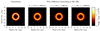 |
Fig. 1. Images of the geometric model of concentric Gaussian rings in the unscattered and diffractive scattering regime at 320 GHz. Here, α is the power-law index of the phase structure function of the scattering screen and rin fixes the inner scale of the turbulence power-law regime. The parameter choices are discussed in Section 2. |
It was recently shown by Tamar & Palumbo (2024) that, for such a geometric model, closed-form expressions exist in total intensity, linear polarization (LP) and circular polarization that can specify the exact point in the Fourier domain where the photon ring signal first begins to dominate. Moreover, an analysis of the sensitivity and antenna diameter requirements by those authors indicates that, for BHEX, accessing photon ring signatures in LP is much more likely than for those from circular polarization. The formula for the LP transition point, (ρT)LP, depends on the aforementioned parameters of the geometric model as well as on the ratio βr = β2, 0/β2, 1, where the β2 coefficient captures the rotationally symmetric polarization structure (Palumbo & Wong 2022). The formula, reproduced from Equation (20) from Tamar & Palumbo (2024), having ℱ = F0/F1 and σ0 and σ1 being the Gaussian thickness for the n = 0 and n = 1 rings respectively, is given by
 (1)
(1)
Substituting the aforementioned parameter values, along with a reasonable value of βr = 3 inferred from Figure 2 of (Palumbo & Wong 2022), Equation (1) gives the transition point of ≈13.5 rmGλ, implying that, under the assumptions of our geometric model, the photon ring signal starts to dominate after 13.5 Gλ. This is consistent with the findings of Palumbo et al. (2023) and would serve as an instructive reference value to gauge the baselines that need to be accessed by BHEX to probe Sgr A*’s photon ring signal. This fact is also represented in Figure 2, wherein it is evident that the ground-based EHT array does not probe long enough baselines to be sensitive to the LP photon ring signal furnished by our model.
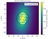 |
Fig. 2. Model of Sgr A*’s diffractive scattering of Sgr A* at 320 GHz based on parameters from J18. Here, ρPR is the approximate (u, v) radius predicted for our putative geometric model, beyond which the photon ring signal is expected to dominate for Sgr A*’s observations at the chosen frequency. The (u, v) coverage in white is of the putative EHT 2025 array (see Table B.1). |
4. Observing Sgr A* with Earth-space VLBI
In this section, we quantify the sensitivity of BHEX baselines with the ground stations to probe the proposed geometric model of Sgr A*’s photon ring, while considering variations in parameters of ISM turbulence across our three sets J (α = 1.38, rin = 800 km), K (α = 1.67, rin = 600 km), and S (α = 1.99, rin = 1000 km).
4.1. Instrumentation considerations: Thermal noise
The sensitivity of a baseline formed by two stations, say i, and j, is measured by the thermal noise, σij, for the baseline that is related to the stations’ system equivalent flux densities (SEFD), bandwidth (Δν), integration time (tint) and quantisation efficiency (η) by the relation,
 (2)
(2)
The SEFD in turn depends on the system temperature (Tsys), antenna efficiency (ηA) and diameter (d) as
 (3)
(3)
where π(d/2)2 represents the antenna area and kB is the Boltzmann constant. For BHEX, assuming Tsys = 50 K, ηA = 0.75, and d = 3.5 m (Johnson et al. 2024), the SEFD value is
 (4)
(4)
For this paper, we considered BHEX’s baselines with three stations: the Atacama Large Millimeter/submillimeter Array (ALMA) in Chile, the Submillimeter Array (SMA) facilities on Maunakea in Hawaii and the Submillimeter Telescope (SMT) in Arizona. These sites were part of the EHT array that in 2017 observed Sgr A* (Event Horizon Telescope Collaboration 2022a) and they are also proposed to be part of the next generation EHT (ngEHT) with expanded multi-frequency capabilities (Doeleman et al. 2023).
Our choice for the sites was governed by quantitative considerations. In particular, since σij is directly proportional to the SEFD at the station, a lower value of the site’s SEFD would imply lesser thermal noise across the baseline thereby enhancing the sensitivity. Among our three sites, ALMA is the most sensitive, followed by SMA and then SMT. This is evident from their SEFD values of
-
SEFD (ALMA) = 74 Jy;
-
SEFD (SMA) = 6700 Jy; and
-
SEFD (SMT) = 10 500 Jy.
These values are taken from the specifications published by the EHT for its 2017 observing campaign (Event Horizon Telescope Collaboration 2019d). As a consequence, the BHEX-ALMA baseline will be the most sensitive in the Earth-space array. We worked with these SEFD values with the implicit assumption that any increase or decrease in SEFD values would decrease or increase the sensitivity of the corresponding baseline.
Next, using these SEFD values for ALMA, SMA and SMT along with the value given in Eq. (4), assuming BHEX observes with a bandwidth of 16 GHz and integration time of 10 seconds, the thermal noise values σBHEX-ALMA, σBHEX-SMA and σBHEX-SMT for our chosen baselines are 2.71 mJy, 25.83 mJy and 32.33 mJy respectively. These σ values would serve as the “floor” such that the amount of signal that can be probed by these baselines must have flux values higher than the detection threshold of 3σ. We note that there is an unfortunate overlap of notation of using σ to represent both, the Gaussian thickness of the rings and the thermal noise of a baseline. Nevertheless, one can refer to the subscripts to clarify the context of their usage; for the discussion on thermal noise floor, σ represents the thermal noise values for the baselines considered above.
4.2. Results
For the BHEX-ALMA, BHEX-SMA, and BHEX-SMT baselines, observations of our model of Sgr A*’s signal are shown in Figure 3. The gray region represents the inaccessible flux that lies below the thermal noise floor for the corresponding baseline. Conversely, the colored region represents the flux that lies above the floor. The red dots represent the (u, v) coverage for the corresponding baseline for 24 hours of observation, sampled at intervals of 60 minutes.
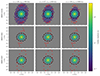 |
Fig. 3. Total flux for the BHEX-ALMA, BHEX-SMA and BHEX-SMT baselines for various values of α and rin. The colored and gray regions represent the accessible and inaccessible flux, with the floor set by the thermal noise for the corresponding baseline. The red dots represent the (u, v) coverage for the baseline and the black circle is at 13.5 Gλ which represents the boundary for our model beyond which the photon ring in linear polarization is expected to dominate. The colored region represents the flux signal lying above the detection threshold of 3σ for each baseline. |
4.2.1. Influence of the scattering parameters
The dependence of the accessible signal on the scattering parameters α and rin is quite evident. For any baseline, horizontally traversing toward higher values of α leads to lower amounts of signal above the thermal noise floor, consequently limiting the ability to observe Sgr A* on the longest baselines. We also checked that the effect of varying rin within our range was not as severe as that from the variations in α. More broadly, this implies that the existing uncertainty over the properties of the ISM turbulence is intimately related to BHEX’s ability to observe Sgr A* and, therefore, requires careful consideration. Furthermore, a column-wise comparison makes it evident that if the model parameters presented by J18 are accurate, a greater quanta of signal is accessible on the longest baselines.
4.2.2. Baseline considerations
From the first row of the Figure, it is encouraging to see that even if we move toward the limiting value of αS = 1.99, the sensitivity of the BHEX-ALMA baseline will continue to probe the region where Sgr A*’s signal persists. Therefore, at least on its most sensitive baseline, for the parameter space being considered in this paper, BHEX should observe Sgr A*.
For the BHEX-SMA and BHEX-SMT baselines, the situation is a little more challenging. Firstly, higher values of α lead to the source flux becoming less accessible to long baseline observations, with the signal sparsity being particularly acute in the BHEX-SMT baseline. However, we note that in both of these cases (and, of course, for the BHEX-ALMA baseline as well), the region until ≈13.5 Gλ continues to have accessible flux. Therefore, we make the inference that for BHEX to work with an array of Earth stations with varying levels of baseline sensitivities, the suitable region of the visibility domain for Sgr A* observations actually lies around 13.5 Gλ. This is shorter than the 20 Gλ baseline lengths currently envisaged by the mission when observing at 320 GHz (Johnson et al. 2024).
Keeping these considerations in mind, in the subsequent sections we lay out a dynamic orbit scheme, quantified by mission design considerations, that can potentially allow BHEX to still go to its proposed final orbit but also pass through and perform observations at intermediate orbits. Such an implementation would provide access regions of the Fourier space identified above that would continue to have an accessible signal for baselines of varying sensitivities, while mitigating the potential loss in signal due to uncertainties in the ISM’s turbulence properties.
5. Orbit transfers and Earth-space VLBI
A space mission has a designated “target” orbit that is chosen to maximize its scientific output. However, it is often the case that the orbiter is not directly injected into that orbit, but is first launched into an initial “parking” orbit from which it performs a series of transfers to go to the target orbit. As an example, the INTEGRAL mission (Winkler et al. 2003) first launched the orbiter into a low, nearly circular parking orbit, then into a highly elliptical transfer orbit and finally into the target geosynchronous orbit (Eismont et al. 2003; Jensen et al. 2003).
For this paper, the target orbit was chosen to be the reference orbit of the BHEX mission (Johnson et al. 2024). This orbit was been preliminarily selected for BHEX for these reasons:
-
The selected altitude provides the required angular resolution on ground-space baselines to probe the photon ring. An orbital period of 12 sidereal hours also generates a repeating ground track of the spacecraft which simplifies selection of ground station locations for data downlinking;
-
the inclination maximises the projected baseline length toward both Sgr A* and M87*; and
-
for M87*, precise estimates of the mass are not available which requires that mass and spin degeneracies in the photon ring must be broken with two-dimensional information about its shape and relative astrometry. This requires near-circular (u,v) coverage by selecting an orbital plane almost perpendicular to M87*. For Sgr A*, knowledge of the mass is available to a finer degree of precision. This means that a photon ring size measurement along even a single axis provides an excellent spin constraint. The orbital plane has, however, been rotated slightly to increase the coverage of Sgr A* in the u-plane.
To reach the target orbit, we propose a “transfer-observe-transfer” orbital migration scheme that starts from a parking orbit that is in the low earth orbit (LEO) region, having a semimajor axis of a = 7000 km. The orbiter performs 1 day of observations in this orbit. Then it goes to two intermediate circular orbits (hereafter IC1 and IC2) having a = 13 000 and a = 19 000 km, respectively, observing for 1 day in each of them. We note that an extended time can be spent in the intermediate orbits if there are any unforeseen challenges to observing on a particular day. Finally, the orbiter goes to the target BHEX orbit and observes for 1 day. Since all the aforementioned orbits are circular, the argument of perigee is an undefined quantity (and taken to be 0°, as per convention) and the true anomaly, ν, is a free parameter. The corresponding orbital parameters for all of these stages are given in Table 1. In the next section, we discuss the two possible astrodynamical methods that can perform the transfer between these orbits.
Orbital parameters for performing an orbit migration from the initial parking orbit to the final target orbit.
5.1. Hohmann transfers
One of the most well-studied orbit transfers is the Hohmann transfer (Vallado 2013). When the ratio of the radii of the initial and final orbits involved in an orbital transfer is low, it is the most energy-efficient transfer between two circular coplanar orbits (Prussing 1992). It utilizes two impulsive thrusts: one at the perigee of the initial orbit that launches the orbiter into an elliptical transfer orbit, and the second at the apogee of this orbit that launches the orbiter into the final orbit. Since the thrusts are impulsive, a large Δv is required from the thruster in a short span of time and, therefore, Hohmann transfers are performed using CP.
It is easy to recognize the utility of the Hohmann transfer for a mission like BHEX whose proposed final orbit is circular and where the standard implementation of the transfer is between circular orbits. However, it is possible that for non-circular parking or intermediate orbits, more sophisticated and fuel-efficient optimization schemes exist. Nevertheless, our motivation for working with the Hohmann transfer was to use it as a tool to demonstrate the construction of a mission architecture that addresses the astrophysical requirement, identified earlier, of making observations at baselines shorter than the ones obtained from BHEX’s final orbit.
A demonstration of the (u, v) coverage for observing Sgr A* based on a series of Hohmann transfers is given in Figure 4. This represents the (u, v) coverage for a space orbiter being added to the expected EHT 2025 array (see Table B.1), with the former supporting an observing bandwidth of 16 GHz and an integration time of t = 10 s (Johnson et al. 2024). For the parking orbit, the time between scans is 900 s, which ensures filling of the (u, v) plane with the orbiter having a relatively short period (≈97 minutes). Although the parking orbit does not access the baseline lengths needed to probe the photon ring signal considered in this paper, it can still be used for checking various subsystems of the orbiter. For IC1, IC2 and the final BHEX orbit this time is chosen to be one-twelfth of the orbital period which comes out to be approximately 20, 36, and 60 minutes respectively). The top panel represents the putative (u, v) coverage obtained using ehtim while the bottom panel shows the coverage generated using the spacevlbi1 tool that models the impact on (u, v) coverage if realistic mission constraints are considered (Hudson 2024). The points in shades of green represent the points lying in the region outside 13.5 Gλ which was identified in Section 3 as the point in the Fourier domain where the LP photon ring signature in LP first begins to dominate.
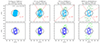 |
Fig. 4. (u, v) coverage of the proposed orbital migration scheme. The temporal and angular resolutions are denoted by tres and θres, respectively, with the corresponding values in gravitational units denoted by the subscript, G. The angle φpr represents the angular sampling of the photon ring at each stage. The top and bottom panel coverage is generated using ehtim and spacevlbi packages, respectively, with the latter imposing the constraint of maintaining a real-time downlink connection with ground stations. The VLBI ground array and the downlink station locations are given in Table B.1. |
5.2. Electric orbit raising
An alternative to the CP-based Hohmann transfer is the EP-based electric orbit raising (EOR). The primary advantage of EP over CP is the significantly higher specific impulse, but that comes at a cost of increased transfer time and typically a much higher power requirement that can drive the spacecraft power system design. Here, the thrust provided in a single burn is significantly lower than CP and hence cannot be used to perform the Hohmann transfer. Moreover, the time taken to go from one orbit to another is significantly longer compared to the Hohmann case. Nevertheless, due to a much higher specific impulse, EP is much more fuel efficient than CP and this can be used to increase the payload mass for a given mission. The relevant formulae to compute the time and fuel required for EOR are given in Section C of the appendix.
We note that the (u, v) coverage for both CP and EP would crudely look the same since the observing campaign is being triggered only on the four orbits in Table 1 and not in between them. However, where propulsion does come into play is the time taken to reach these orbits and the fuel that would be required to perform these orbital maneuvers. This will be discussed in the next section.
6. Impact of practical mission considerations on Earth-space VLBI
We now discuss the impact on Earth-space VLBI observations of two crucial mission design considerations for BHEX, namely maintaining a real-time downlink connection with ground stations, and the choice of propulsion.
6.1. Maintaining a real-time downlink connection
In performing VLBI observations from space, there are a number of potential limitations on when observations can be performed, imposed by the spacecraft and wider mission design. These are hereafter called functional constraints which in general include (but are not limited to):
-
Sun, Earth and Moon blinding of star trackers required for high accuracy attitude control;
-
radiator surfaces not being deep-space pointed as required for the demanding thermal control of space VLBI missions; and
-
tracking of the spacecraft for highly accurate orbit determination required for the correlation process.
For BHEX, a major constraint is the preliminary decision to perform real-time downlinking of science data to a network of ground stations via an optical link (Wang et al. 2024). Alternatives to this solution, including the use of mass data storage onboard the spacecraft were evaluated. However, we determine that the technology readiness of data storage to the level required for BHEX is not sufficiently mature for inclusion in a Small Explorers (SMEX) mission. Such technologies also come with a significant mass and power requirement. The use of an optical terminal to achieve real-time downlink of the large volumes of data is deemed to be more feasible within the tight constraints of the mission. The difficulties associated with this choice are noted and future work will explore these challenges and propose solutions.
The impact of this constraint is that observations cannot be performed at times when a link between the spacecraft’s optical terminal and the network of ground stations is not possible. Various parameters impact the severity of this constraint, including: the attitude control strategy of the spacecraft, the specific ground station configuration, the minimum elevation of the spacecraft at the optical ground stations, and the gimbal control limits of the onboard optical terminal.
To study the impact of this constraint on Sgr A*’s observations, in Figure 4, the second panel depicts the potential impact on (u, v) coverage caused by the inability to maintain a real-time downlink throughout the spacecraft’s orbit. The chosen downlink stations are specified in Table B.1, with station choices driven by the potential sites identified by BHEX (Wang et al. 2024). Final selection of the BHEX optical ground station sites is still taking place, considering factors such as orbit coverage, budget, and the viability of the site (e.g., weather, technology readiness). This panel, generated using spacevlbi, enables modeling of the major functional constraints impacting a space-based VLBI mission. The implementation in the package includes the effect of Earth’s obscuration and the constraint of maintaining a real-time downlink with Earth-based stations. For this example case, an optical terminal with a ±90° gimbal control mechanism was implemented on the spacecraft. Throughout observations, the science antenna was pointed at Sgr A*. The spacecraft’s attitude was, however, however rotated about the science antenna direction every half-orbit period to keep the optical terminal approximately pointed toward the Earth.
The impact on observations and, thus, the science return on the mission can be seen in the loss of (u, v) coverage between the top and bottom panels of Figure 4. This is more pronounced for lower-altitude orbits, as four ground stations are not sufficient to provide full coverage of a spacecraft in LEO. However, we note that a different choice of mean anomaly (which signifies the time at which the orbiter is launched) can lead to a dramatically different downlink coverage in the LEO, thereby giving more (u, v) points at this altitude. Indeed, the choice of mean anomaly for this paper was to optimize the coverage with respect to ground for the final BHEX orbit, but that has no bearing on the values for the lower orbits. Mitigating the impact of the functional constraints is crucial for maximizing the science return of a mission and, and for BHEX, the real-time downlink is likely to be the dominant factor.
6.2. Impact of propulsion choices
To make the propulsion computations for our orbit migration scheme, we made the following choices. The propellant requirements for CP were chosen based on Falcon 9’s specifications, which have been NASA’s choice for the SMEX class of missions like IXPE (Weisskopf et al. 2022), launched in 2021, while EP’s expellant parameters are of the SPT-140 Hall thrusters that were recently used by NASA in the Discovery class Psyche mission (Hart et al. 2018; Khan et al. 2024), launched in 2023. We note that BHEX is a proposed SMEX class mission and would therefore use a smaller version of the Psyche propulsion system design. The performance parameters for these propellants, along with the detailed computations for the time and fuel requirements for implementing the transfers, are given in Appendix C.
6.3. Results and inferences
We find that, assuming a spacecraft dry mass of 300 kg (a typical upper limit on NASA SMEX missions (Smith 2024), for CP-based Hohmann transfer using cryogenic liquid methane and liquid oxygen (LOX) as a propellant, it would require 195.889 kg of fuel and 9.21 hours to go from the parking to the target orbit through our bespoke orbital scheme. For an EP-based EOR using the SPT-140 Hall effect thruster, it would require 57.20 kg of fuel and 44.2 days to complete the migration.
The significantly large amount of fuel required for the Hohmann transfer-based scheme restricts its practical utility for having an orbiter observe in the intermediate stage, at least in the context of the budget constraints of the SMEX mission. The high propellant mass would require a launch vehicle upper stage (like the Falcon 9 Block 5) or a kick stage rocket to perform the transfer. Utilization of such a system would make it highly unlikely that observations could be performed by BHEX during the transfer as this would require the attitude control system to be designed to accommodate connection to this upper stage, resulting in an overdesigned system for the nominal mission.
On the other hand, the values obtained from EP are encouraging, since not only are the fuel requirements significantly lower than the CP case (which is expected), but also the total migration time of 44 days is not prohibitively long with respect to BHEX’s 2-year mission (Johnson et al. 2024), which is often one of the criticisms of using EP. However, it is noted that EP has an extremely high power requirement (the stated SPT-140 system requires 4.5 kW). Utilization of such a system for BHEX would drive the power system design, resulting in the need for very large solar panels. This may be prohibited by the constraints of an SMEX-class mission. As such, in reality, a smaller, lower-thrust EP system would likely be implemented, resulting in a longer transfer time (see Figure C.1).
7. Consequences for Sgr A*
Changes in the spacecraft orbit change the temporal and spatial resolution of the full VLBI array containing the orbiter. The spatial resolution element of the array can be estimated in a number of ways (Thompson et al. 2017), but is generally inversely proportional to the longest baseline and estimated with
 (5)
(5)
where B is the physical length of the baseline.
However, the temporal resolution element is less clearly defined. Palumbo et al. (2019) used filling of the (u, v) to define an imaging-focused temporal resolution. However, in VLBI applications targeting features varying widely in spatial scale, the uniform (u, v) sampling weight is less sensible.
In this paper, we simply define the temporal resolution afforded by the spacecraft to be one-quarter of its orbital period. Due to the complex conjugate symmetry of the (u, v) plane, a dish in a circular orbit samples essentially all of its (u, v) track in half of its orbit, and so a quarter period represents accruing more than half of the image information at the spatial scales targeted by the orbiter:
 (6)
(6)
For the photon ring morphological science targeted by the BHEX mission, azimuthal angle sampling in the (u, v) plane is also important, as different baseline orientations project out different information about photon ring morphology (Bracewell 1956; Gralla et al. 2020). This angular sampling must occur on baselines not dominated by the direct image structure. To characterize the thoroughness of this sampling over the course of several transfers, we characterized the angular sampling of the photon ring as φpr, the widest range of (u, v) angles sampled by a non-conjugate-redundant subset of the u − v coverage beyond the minimum photon ring (u, v) radius, in this case 13.5 Gλ.
Figure 4 shows three diagnostic properties along with the evolving orbit: the temporal resolution, tres, the spatial resolution, θres, and the angular sampling beyond the photon ring, φpr. The figure also contains values obtained in gravitational units (denoted by the subscript G). These required fixing the mass and distance from Earth of Sgr A* and we considered the values to be MS = 4.1 × 10⁶ M⊙ and DS = 8.1 kpc, respectively (GRAVITY Collaboration 2018). Then, the quantities tG and θG were obtained by dividing tres and θres by GMS/c3 and GMS/c2DS, respectively, where G is Newton’s gravitational constant and c is the speed of light. The quantity GMS/c2DS corresponds to one gravitational radius and serves as a useful unit in constructing quantities sensitive to strong field gravity signatures of Sgr A* (Psaltis et al. 2015). From the values obtained for each stage, we note that raising the orbit worsens the temporal resolution, but improves the spatial resolution and angular sampling of the photon ring.
Each transfer sacrifices more signal to scattering while plumbing finer structures in the source. Depending on the accretion and interstellar scattering conditions in Sgr A*, any of the latter three orbits may be sufficient or even optimal for measuring the spin of Sgr A*, as lower orbits place coverage in regions with detectable signal in Figure 3.
8. Conclusion and future work
For this paper, we have studied the extent to which diffractive scattering affects Earth-space VLBI observations of Sgr A*, focusing primarily on the BHEX mission. A simple geometric model for concentric Gaussian rings was considered for modeling Sgr A*’s photon ring signature, and the effects of diffractive scattering were studied by varying the power-law index, α, of the phase structure function and the inner scale for the onset of turbulence, rin. Through thermal noise calculations, it is shown that, for variations of α from 1.38 to 1.99 and rin from 600 to 1000 km, for the most sensitive baseline, namely BHEX-ALMA, the longest baselines of the orbiter will be sensitive to Sgr A*’s signal. However, for baselines with moderate sensitivity, such as BHEX-SMA and BHEX-SMT, the longest baselines are unable to probe the signal, with the situation getting significantly worse for higher values of α.
These lessons were used to inform a dynamic orbit migration scheme for the mission, wherein instead of just observing in the fixed final orbit, the orbiter goes through two intermediate orbits and observes in each of them. The (u, v) coverage in these orbits will lie in regions where the sensitivity requirements are not prohibitive to observations, while also being robust to variations in α and rin.
Some of the main detailed mission design considerations for this implementation were also studied. We have discussed the importance of including the constraint of maintaining a downlink connection with Earth stations and generated the corresponding (u, v) coverage. For the orbit migration, the Hohmann transfer was presented as a viable option. Subsequently, a quantitative study of the fuel requirements for both CP and EP was conducted, focusing on currently used technologies by NASA’s missions and associated launch vehicles. Lastly, the utility of these orbits to probe Sgr A*’s rapid timescales and photon ring signatures was explored using spatial and temporal resolution estimates, as well as angular sampling of the photon ring signal.
The BHEX mission concept currently requires the study of the M87* and Sgr A* photon rings using the same orbit; these two sources give a trade space for which the target BHEX orbit is one of many reasonable compromises. However, were Sgr A* the only target, the Fourier coverage indicates that slightly shorter baselines may be preferred. While a mission window with shorter baselines can, in principle, be done in a few hours by a CP-based Hohmann transfer scheme using the LOX propellant, the corresponding fuel requirement is prohibitively excessive. On the other hand, EP-based EOR using the SPT-140 thrusters provides a viable mechanism of reaching and observing in the transfer orbits in a fuel efficient manner, requiring comparatively less fuel but also reaching the target BHEX orbit in about 6 weeks. As the science case for the BHEX mission is developed, it will be interesting to explore whether any of these considerations can aid in achieving its scientific goals, particularly for observing Sgr A*. More broadly, it seems that more probably than not, a hybrid propulsion scheme (Mailhe & Heister 2002) might be best-suited for future Earth-space VLBI missions primarily focused on studying Sgr A*.
In future work, we aim to perform a detailed study of how Earth-space VLBI observations of the Galactic Center can help address the uncertainties in various physical processes characterizing turbulence in the ISM.
Acknowledgments
The authors are grateful to the anonymous referee, whose feedback played a pivotal role in obtaining the results presented in this paper. We would also like to thank Michael D. Johnson and Sara Issaoun for several fruitful discussions and Leonid Gurvits for providing valuable comments that helped improve this paper. A.T. gratefully acknowledges the Center for Astrophysics | Harvard & Smithsonian, and the Black Hole Initiative at Harvard University for providing a stimulating environment during an extended research visit between May and July 2024 during which a part of this work was done.
References
- Andrianov, A. S., Baryshev, A. M., Falcke, H., et al. 2021, MNRAS, 500, 4866 [Google Scholar]
- Armstrong, J. W., Rickett, B. J., & Spangler, S. R. 1995, ApJ, 443, 209 [Google Scholar]
- Bhat, N. D. R., Cordes, J. M., Camilo, F., Nice, D. J., & Lorimer, D. R. 2004, ApJ, 605, 759 [CrossRef] [Google Scholar]
- Bower, G. C., Markoff, S., Dexter, J., et al. 2015, ApJ, 802, 69 [Google Scholar]
- Bracewell, R. N. 1956, Aust. J. Phys., 9, 198 [NASA ADS] [Google Scholar]
- Broderick, A. E., Tiede, P., Pesce, D. W., & Gold, R. 2022, ApJ, 927, 6 [NASA ADS] [CrossRef] [Google Scholar]
- Cárdenas-Avendaño, A., & Lupsasca, A. 2023, Phys. Rev. D, 108, 064043 [Google Scholar]
- Cárdenas-Avendaño, A., Lupsasca, A., & Zhu, H. 2023, Phys. Rev. D, 107, 043030 [CrossRef] [Google Scholar]
- Chepurnov, A., & Lazarian, A. 2010, ApJ, 710, 853 [NASA ADS] [CrossRef] [Google Scholar]
- Cho, I., Zhao, G.-Y., Kawashima, T., et al. 2022, ApJ, 926, 108 [NASA ADS] [CrossRef] [Google Scholar]
- Cordes, J. M., & Wolszczan, A. 1986, ApJ, 307, L27 [Google Scholar]
- Cordes, J. M., Weisberg, J. M., & Boriakoff, V. 1985, ApJ, 288, 221 [NASA ADS] [CrossRef] [Google Scholar]
- Cordes, J. M., Pidwerbetsky, A., & Lovelace, R. V. E. 1986, ApJ, 310, 737 [Google Scholar]
- Davies, R. D., Walsh, D., & Booth, R. S. 1976, MNRAS, 177, 319 [NASA ADS] [Google Scholar]
- Doeleman, S. S., Barrett, J., Blackburn, L., et al. 2023, Galaxies, 11, 107 [NASA ADS] [CrossRef] [Google Scholar]
- Eismont, N. A., Ditrikh, A. V., Janin, G., et al. 2003, A&A, 411, L37 [NASA ADS] [CrossRef] [EDP Sciences] [Google Scholar]
- Event Horizon Telescope Collaboration (Akiyama, K., et al.) 2019a, ApJ, 875, L1 [Google Scholar]
- Event Horizon Telescope Collaboration (Akiyama, K., et al.) 2019b, ApJ, 875, L4 [Google Scholar]
- Event Horizon Telescope Collaboration (Akiyama, K., et al.) 2019c, ApJ, 875, L6 [Google Scholar]
- Event Horizon Telescope Collaboration (Akiyama, K., et al.) 2019d, ApJ, 875, L2 [Google Scholar]
- Event Horizon Telescope Collaboration (Akiyama, K., et al.) 2021, ApJ, 910, L13 [Google Scholar]
- Event Horizon Telescope Collaboration (Akiyama, K., et al.) 2022a, ApJ, 930, L12 [NASA ADS] [CrossRef] [Google Scholar]
- Event Horizon Telescope Collaboration (Akiyama, K., et al.) 2022b, ApJ, 930, L14 [NASA ADS] [CrossRef] [Google Scholar]
- Event Horizon Telescope Collaboration (Akiyama, K., et al.) 2024a, ApJ, 964, L25 [NASA ADS] [CrossRef] [Google Scholar]
- Event Horizon Telescope Collaboration (Akiyama, K., et al.) 2024b, A&A, 681, A79 [NASA ADS] [CrossRef] [EDP Sciences] [Google Scholar]
- Filothodoros, A., Lewandowski, W., Kijak, J., et al. 2024, MNRAS, 528, 5667 [Google Scholar]
- Fish, V. L., Shea, M., & Akiyama, K. 2020, Adv. Space Res., 65, 821 [Google Scholar]
- Fromm, C. M., Mizuno, Y., Younsi, Z., et al. 2021, A&A, 649, A116 [NASA ADS] [CrossRef] [EDP Sciences] [Google Scholar]
- Gabányi, K. É., Krichbaum, T. P., Britzen, S., et al. 2006, A&A, 451, 85 [NASA ADS] [CrossRef] [EDP Sciences] [Google Scholar]
- Ghez, A. M., Salim, S., Weinberg, N. N., et al. 2008, ApJ, 689, 1044 [Google Scholar]
- Goddi, C., Martí-Vidal, I., Messias, H., et al. 2021, ApJ, 910, L14 [NASA ADS] [CrossRef] [Google Scholar]
- Goldreich, P., & Sridhar, S. 1995, ApJ, 438, 763 [Google Scholar]
- Goodman, J., & Narayan, R. 1989, MNRAS, 238, 995 [Google Scholar]
- Gralla, S. E., & Lupsasca, A. 2020, Phys. Rev. D, 102, 124003 [NASA ADS] [CrossRef] [Google Scholar]
- Gralla, S. E., Lupsasca, A., & Marrone, D. P. 2020, Phys. Rev. D, 102, 124004 [NASA ADS] [CrossRef] [Google Scholar]
- GRAVITY Collaboration (Abuter, R., et al.) 2018, A&A, 615, L15 [NASA ADS] [CrossRef] [EDP Sciences] [Google Scholar]
- GRAVITY Collaboration (Abuter, R., et al.) 2019, A&A, 625, L10 [NASA ADS] [CrossRef] [EDP Sciences] [Google Scholar]
- Gupta, Y., Rickett, B. J., & Coles, W. A. 1993, ApJ, 403, 183 [NASA ADS] [CrossRef] [Google Scholar]
- Gurvits, L. I. 2020, Adv. Space Res., 65, 868 [NASA ADS] [CrossRef] [Google Scholar]
- Gwinn, C. R., Kovalev, Y. Y., Johnson, M. D., & Soglasnov, V. A. 2014, ApJ, 794, L14 [Google Scholar]
- Hart, W., Brown, G. M., Collins, S. M., et al. 2018, 2018 IEEE Aerospace Conference, 1 [Google Scholar]
- Hudson, B. 2024, Python Package for Simulating and Optimising aSpace-based VLBI Mission, Language: en Medium: Python Package [Google Scholar]
- Hudson, B., Gurvits, L. I., Wielgus, M., et al. 2023, Acta Astron., 213, 681 [Google Scholar]
- Issaoun, S., Johnson, M. D., Blackburn, L., et al. 2019, ApJ, 871, 30 [Google Scholar]
- Jensen, P. L., Clausen, K., Cassi, C., et al. 2003, A&A, 411, L7 [NASA ADS] [CrossRef] [EDP Sciences] [Google Scholar]
- Jiménez-Rosales, A., Dexter, J., Ressler, S. M., et al. 2021, MNRAS, 503, 4563 [CrossRef] [Google Scholar]
- Johnson, M. D. 2016, ApJ, 833, 74 [Google Scholar]
- Johnson, M. D., & Gwinn, C. R. 2015, ApJ, 805, 180 [NASA ADS] [CrossRef] [Google Scholar]
- Johnson, M. D., & Narayan, R. 2016, ApJ, 826, 170 [Google Scholar]
- Johnson, M. D., Narayan, R., Psaltis, D., et al. 2018, ApJ, 865, 104 [NASA ADS] [CrossRef] [Google Scholar]
- Johnson, M. D., Lupsasca, A., Strominger, A., et al. 2020, Sci. Adv., 6, eaaz1310 [NASA ADS] [CrossRef] [Google Scholar]
- Johnson, M. D., Kovalev, Y. Y., Lisakov, M. M., et al. 2021, ApJ, 922, L28 [CrossRef] [Google Scholar]
- Johnson, M. D., Akiyama, K., Baturin, R., et al. 2024, ArXiv e-prints [arXiv:2406.12917] [Google Scholar]
- Khan, S., Lawler, C., Nicholas, A., et al. 2024, 2024 IEEE Aerospace Conference, 1 [Google Scholar]
- Koryukova, T. A., Pushkarev, A. B., Plavin, A. V., & Kovalev, Y. Y. 2022, MNRAS, 515, 1736 [NASA ADS] [CrossRef] [Google Scholar]
- Lambert, H. C., & Rickett, B. J. 2000, ApJ, 531, 883 [NASA ADS] [CrossRef] [Google Scholar]
- Likhachev, S. F., Rudnitskiy, A. G., Shchurov, M. A., et al. 2022, MNRAS, 511, 668 [Google Scholar]
- Lo, K. Y., Backer, D. C., Kellermann, K. I., et al. 1993, Nature, 362, 38 [Google Scholar]
- Mailhe, L. M., & Heister, S. D. 2002, Journal of Spacecraft and Rockets, 39, 131 [Google Scholar]
- Narayan, R., & Goodman, J. 1989, MNRAS, 238, 963 [NASA ADS] [Google Scholar]
- Özel, F., Psaltis, D., & Younsi, Z. 2022, ApJ, 941, 88 [CrossRef] [Google Scholar]
- Palumbo, D. C. M., & Wong, G. N. 2022, ApJ, 929, 49 [Google Scholar]
- Palumbo, D. C. M., Doeleman, S. S., Johnson, M. D., Bouman, K. L., & Chael, A. A. 2019, ApJ, 881, 62 [Google Scholar]
- Palumbo, D. C. M., Wong, G. N., Chael, A., & Johnson, M. D. 2023, ApJ, 952, L31 [Google Scholar]
- Prussing, J. E. 1992, J. Guidance Control Dyn., 15, 1037 [Google Scholar]
- Psaltis, D., Özel, F., Chan, C.-K., & Marrone, D. P. 2015, ApJ, 814, 115 [Google Scholar]
- Psaltis, D., Johnson, M., Narayan, R., et al. 2018, ArXiv e-prints [arXiv:1805.01242] [Google Scholar]
- Pushkarev, A. B., Kovalev, Y. Y., Lister, M. L., et al. 2013, A&A, 555, A80 [NASA ADS] [CrossRef] [EDP Sciences] [Google Scholar]
- Raymond, A. W., Doeleman, S. S., Asada, K., et al. 2024, AJ, 168, 130 [NASA ADS] [CrossRef] [Google Scholar]
- Ricarte, A., & Dexter, J. 2015, MNRAS, 446, 1973 [Google Scholar]
- Roelofs, F., Falcke, H., Brinkerink, C., et al. 2019, A&A, 625, A124 [NASA ADS] [CrossRef] [EDP Sciences] [Google Scholar]
- Shavelle, K. M., & Palumbo, D. C. M. 2024, ApJ, 970, L24 [Google Scholar]
- Shlentsova, A., Roelofs, F., Issaoun, S., Davelaar, J., & Falcke, H. 2024, A&A, 686, A154 [NASA ADS] [CrossRef] [EDP Sciences] [Google Scholar]
- Smirnova, T. V., Shishov, V. I., Popov, M. V., et al. 2014, ApJ, 786, 115 [NASA ADS] [CrossRef] [Google Scholar]
- Smith, D. 2024, Astrophysics and Heliophysics Explorers Program [Google Scholar]
- Tamar, A., & Palumbo, D. C. M. 2024, ApJ, 977, 147 [Google Scholar]
- Tamar, A., Hudson, B., & Palumbo, D. C. M. 2024, ApJ, 967, 90 [Google Scholar]
- The Event Horizon Telescope Collaboration 2024, ArXiv e-prints [arXiv:2410.02986] [Google Scholar]
- Thompson, A. R., Moran, J. M., & Swenson, G. W., Jr 2017, Interferometry and Synthesis in Radio Astronomy, 3rd edn. (Springer Open) [CrossRef] [Google Scholar]
- Tiede, P., Johnson, M. D., Pesce, D. W., et al. 2022, Galaxies, 10, 111 [NASA ADS] [CrossRef] [Google Scholar]
- Trippe, S., Jung, T., Lee, J. W., et al. 2023, ArXiv e-prints [arXiv:2304.06482] [Google Scholar]
- Tuntsov, A. V., Bignall, H. E., & Walker, M. A. 2013, MNRAS, 429, 2562 [Google Scholar]
- Vallado, D. A. 2013, Fundamentals of Astrodynamics, 4th edn. (Microcosm Press) [Google Scholar]
- Wang, J., Bilyeu, B., Boroson, D., et al. 2024, ArXiv e-prints [arXiv:2406.09572] [Google Scholar]
- Weisskopf, M. C., Soffitta, P., Baldini, L., et al. 2022, J. Astron. Telesc. Instrum. Sys., 8, 026002 [Google Scholar]
- Winkler, C., Courvoisier, T. J. L., Di Cocco, G., et al. 2003, A&A, 411, L1 [NASA ADS] [CrossRef] [EDP Sciences] [Google Scholar]
- Xu, S., & Zhang, B. 2020, ApJ, 898, L48 [Google Scholar]
- Yuan, F., Wang, H., & Yang, H. 2022, ApJ, 924, 124 [NASA ADS] [CrossRef] [Google Scholar]
- Zhu, Z., Johnson, M. D., & Narayan, R. 2019, ApJ, 870, 6 [Google Scholar]
Appendix A: Terminology
The contents of this paper lie at the intersection of space mission design and astrophysical considerations pertinent to VLBI observations. Therefore, to improve accessibility, a simplified description of the key terms is given in Table A.1.
A glossary of the key terms and mathematical quantities used in the paper.
Appendix B: Ground array stations
The Earth Centered Inertial (ECI) coordinates (X, Y, Z) of the ground stations as part of the putative EHT 2025 array that are used to generate the (u, v) coverage are given in Table B.1.
Appendix C: Orbit transfers and fuel budget considerations
The paper considers two propulsion choices, namely CP and EP. As mentioned in the main text, in order for our results to be of relevance to technologies already being used in missions by NASA, we consider a cryogenic liquid methane and liquid oxygen (LOX) propellant for studying the Hohmann transfer via CP and the 4.5 kW SPT-140 Hall effect thruster which uses Xenon as a propellant, for an electric orbit raising (EOR) scheme. The CP transfer is envisaged to be performed using Falcon 9 Block 5 vehicle, which is the vehicle widely used in NASA’s SMEX class missions.
C.1. Chemical propulsion
Now, for the CP propulsion specifications, there are two main parameters of interest: the specific impulse Isp (usually measured in seconds (s)) which measures the efficiency of an engine to convert propellant to thrust, and Δv (measured in km/s), which is the change in velocity required to perform the maneuver. For specified propellant, the Isp is 348s. Each of the orbit transfers are modelled as a Hohmann transfer and the Δv for each of them is obtained using the Maneuver class of the Python package poliastro2. Rounded up to three decimal places, these are:
 (C.1)
(C.1)
wherein the subscripts denote the semi-major axes (in powers of 103 km) between which the transfer is taking place, with BX being a = 26563.88km for the BHEX mission. The total Δv for the Hohmann transfer, denoted by Δvt, H, is then given by,
 (C.2)
(C.2)
Then, if m0 is the initial mass of the payload with the propellant (“wet mass”) and mf is the final mass without the propellant (“dry mass”), then using the parameters given above, the latter can be computed from the former using the ideal rocket equation (Vallado 2013),
 (C.3)
(C.3)
where g = 9.81m/s2 is the standard gravitational acceleration. Thereafter, total propellant fuel required to perform the transfer is given by,
 (C.4)
(C.4)
For this paper, we consider m0 = 300kg, which is around the maximum payload permissible in NASA’s SMEX class missions. Finally, using this dry mass in the rocket Equation C.3 along with the specified propellant Isp value, we can compute mf for the total Δv given in C.2. The propellant required for each maneuver is then given by Equation C.4. Performing this analysis gives us the total propellant mtot, H required for going from the Parking to the target orbit using three Hohmann transfers:
 (C.5)
(C.5)
For subsequent comparison with the EP case, we also note the total time ttot, H required in performing the three Hohmann transfers, obtained once again using the Maneuver class of poliastro:
C.2. Electric propulsion
Since EP is not an impulsive burn rather a continuous thrust operation, the rocket Equation C.3 does not hold exactly. Now, for a given electric propulsion thrust F and Isp, we first define the initial acceleration a𝒯, I and the specific mass flow rate,
 (C.6)
(C.6)
 (C.7)
(C.7)
Then, for an initial orbit with radius r0 and period T0, and final orbit with radius rf, the accumulated Δv in terms of the ratio R = r1/r0 is given by,
 (C.8)
(C.8)
Finally, the total transfer time is given by Equation 6-44 of Vallado (2013),
 (C.9)
(C.9)
This total time can then be used to compute the total mass mf of propellant required through the equation,
 (C.10)
Now, using Equation C.9, the time taken to transfer from r0 = 7000km to r1 = 26563.88km assuming the SPT-140 parameters of Isp = 1770s and FT = 0.26N, is:
 (C.11)
The coordinates in an ECI frame of the VLBI ground array and the downlink stations used to obtain the (u, v) coverage.
Then, the total propellant mass required, using Equation C.10, is:
 (C.12)
From the propellant requirements obtained in Equations C.5 and C.12, it is patently evident that EP leads to significant improvement in the overall fuel budget of the mission. However, as can be noted from comparing the time required for performing the CP-based Hohmann transfer and the EP-based EoR, the savings in propellant mass comes at a cost of relatively longer transfer time. Lastly, Figure C.1 plots the total time taken to achieve a given orbital radius for varying values of the specific thrust FT. It is evident that as FT increases, the transfer time reduces. Since SPT-140 has a relatively higher FT, it has a reasonable transfer time of 44.2 days to reach the proposed BHEX target orbit with radius rBX = 26563.88 km.
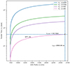 |
Fig. C.1. The total transfer time taken for an EP-based orbit raising for various values of specific thrust FT, as a function of orbital radius. A fixed value of Isp = 1770s is chosen which, along with FT = 0.26N are the specifications of the SPT-140 thruster. The time tt, BX is the time required to perform the orbit migration scheme of Parking→IC1→IC2→target developed in this paper. |
The specific impulse parameter (Isp) deserves some clarification since its units of seconds might seem a little confusing. Simply, specific impulse measures the efficiency of an engine by computing how much thrust it can produce per unit of the propellant. In particular, the phrase “specific” here means divided by the weight (w) (of the fuel) and the quantity being divided is the impulse I of the thruster, with the usual units of Newtons-second. This impulse is defined in terms of the mass of the fuel being expelled and the effective exhaust velocity of the thruster (Vallado 2013) but for the current discussions, these specifications are not necessary; we just need to recall the SI units of impulse. Thus, using standard dimensional analysis, we can obtain the dimensions of Isp as:
![Mathematical equation: $$ \begin{aligned}{[I_{sp}]}=\frac{[I]}{[w]}=\frac{MLT^{-1}}{MLT^{-2}}=T \end{aligned} $$](/articles/aa/full_html/2025/07/aa52668-24/aa52668-24-eq21.gif) (C.13)
(C.13)
with T being the time dimension which in SI units is measured in seconds.
All Tables
Orbital parameters for performing an orbit migration from the initial parking orbit to the final target orbit.
The coordinates in an ECI frame of the VLBI ground array and the downlink stations used to obtain the (u, v) coverage.
All Figures
|
Fig. 1. Images of the geometric model of concentric Gaussian rings in the unscattered and diffractive scattering regime at 320 GHz. Here, α is the power-law index of the phase structure function of the scattering screen and rin fixes the inner scale of the turbulence power-law regime. The parameter choices are discussed in Section 2. |
| In the text | |
|
Fig. 2. Model of Sgr A*’s diffractive scattering of Sgr A* at 320 GHz based on parameters from J18. Here, ρPR is the approximate (u, v) radius predicted for our putative geometric model, beyond which the photon ring signal is expected to dominate for Sgr A*’s observations at the chosen frequency. The (u, v) coverage in white is of the putative EHT 2025 array (see Table B.1). |
| In the text | |
|
Fig. 3. Total flux for the BHEX-ALMA, BHEX-SMA and BHEX-SMT baselines for various values of α and rin. The colored and gray regions represent the accessible and inaccessible flux, with the floor set by the thermal noise for the corresponding baseline. The red dots represent the (u, v) coverage for the baseline and the black circle is at 13.5 Gλ which represents the boundary for our model beyond which the photon ring in linear polarization is expected to dominate. The colored region represents the flux signal lying above the detection threshold of 3σ for each baseline. |
| In the text | |
|
Fig. 4. (u, v) coverage of the proposed orbital migration scheme. The temporal and angular resolutions are denoted by tres and θres, respectively, with the corresponding values in gravitational units denoted by the subscript, G. The angle φpr represents the angular sampling of the photon ring at each stage. The top and bottom panel coverage is generated using ehtim and spacevlbi packages, respectively, with the latter imposing the constraint of maintaining a real-time downlink connection with ground stations. The VLBI ground array and the downlink station locations are given in Table B.1. |
| In the text | |
|
Fig. C.1. The total transfer time taken for an EP-based orbit raising for various values of specific thrust FT, as a function of orbital radius. A fixed value of Isp = 1770s is chosen which, along with FT = 0.26N are the specifications of the SPT-140 thruster. The time tt, BX is the time required to perform the orbit migration scheme of Parking→IC1→IC2→target developed in this paper. |
| In the text | |
Current usage metrics show cumulative count of Article Views (full-text article views including HTML views, PDF and ePub downloads, according to the available data) and Abstracts Views on Vision4Press platform.
Data correspond to usage on the plateform after 2015. The current usage metrics is available 48-96 hours after online publication and is updated daily on week days.
Initial download of the metrics may take a while.