| Issue |
A&A
Volume 698, June 2025
|
|
|---|---|---|
| Article Number | A244 | |
| Number of page(s) | 14 | |
| Section | Astronomical instrumentation | |
| DOI | https://doi.org/10.1051/0004-6361/202554152 | |
| Published online | 20 June 2025 | |
Broadband polarized radio emission detected from Starlink satellites below 100 MHz with NenuFAR
1
LIRA, Observatoire de Paris, Université PSL, Sorbonne Université, Université Paris Cité, CY Cergy Paris Université, CNRS,
92190
Meudon,
France
2
Observatoire Radioastronomique de Nançay (ORN), Observatoire de Paris, Université PSL, Univ Orléans, CNRS,
18330
Nançay,
France
3
ASTRON, Netherlands Institute for Radio Astronomy,
Oude Hoogeveensedijk 4,
7991 PD
Dwingeloo,
The Netherlands
4
LUX, Observatoire de Paris, Université PSL, Sorbonne Université, CNRS,
75014
Paris,
France
5
LPC2E, OSUC, Univ Orléans, CNRS, CNES, Observatoire de Paris,
45071
Orléans,
France
6
Department of Astronomy and Carl Sagan Institute, Cornell University,
Ithaca,
NY,
USA
7
IRA NASU, Institute of radio astronomy of NAS of Ukraine,
Kharkiv,
Ukraine
8
Kapteyn Astronomical Institute, University of Groningen,
PO Box 800,
9700 AV
Groningen,
The Netherlands
9
LOFAR ERIC,
Oude Hoogeveensedijk 4,
Dwingeloo,
The Netherlands
10
Université Paris Cité and Université Paris Saclay, CEA, CNRS, AIM,
91190
Gif-sur-Yvette,
France
★ Corresponding author: This email address is being protected from spambots. You need JavaScript enabled to view it.
Received:
17
February
2025
Accepted:
11
April
2025
Abstract
Aims. We evaluate the impact of Starlink satellites on low-frequency radio astronomy below 100 MHz. We focus on challenges of the data processing and on scientific goals.
Methods. We conducted 40 hours of imaging observations using NenuFAR in the 30.8–78.3 MHz range. Observations included both the targeted tracking of specific satellites based on orbital predictions and the untargeted searches focused on high-elevation regions of the sky. Images in total intensity and polarimetry were obtained, and full Stokes dynamic spectra were generated for several hundred directions within the field of view. The detected signals were cross-matched with satellite orbital data to confirm the satellite associations. We performed detailed analyses of the observed spectra, polarization, and temporal characteristics to investigate the origin and properties of the detected emissions.
Results. We detected broadband emissions from Starlink satellites, predominantly between 54–66 MHz, with flux densities exceeding 500 Jy. These signals are highly polarized and unlikely to originate from ground-based radio frequency interference or reflected astronomical sources. Instead, they are likely intrinsic to the satellites, and distinct differences in the emission properties are observed for the different satellite generations. These findings highlight significant challenges to the data processing and scientific discoveries at these low frequencies and emphasize the need for effective mitigation strategies, in particular, through collaboration between astronomers and satellite operators.
Key words: polarization / space vehicles / techniques: interferometric / radio continuum: general
© The Authors 2025
 Open Access article, published by EDP Sciences, under the terms of the Creative Commons Attribution License (https://creativecommons.org/licenses/by/4.0), which permits unrestricted use, distribution, and reproduction in any medium, provided the original work is properly cited.
This article is published in open access under the Subscribe to Open model. This email address is being protected from spambots. You need JavaScript enabled to view it. to support open access publication.
1 Introduction
Satellite contamination has long been a significant concern for astronomical observations at various wavelengths. In optical astronomy, the satellites that orbit Earth reflect sunlight, which creates bright streaks or flares in telescope images. A notable example is the iridium flare, which can be as bright as magnitude −8 (Hainaut & Williams 2020). In radio astronomy, global navigation satellite system (GNSS) satellites are known to contribute to the radio frequency interference (RFI), probably through out-of-band emissions, harmonics, or intermodulation products (Wildemeersch & Fortuny-Guasch 2010). Additionally, satellites residing in low-Earth orbit (LEO) can reflect ground-based RFI back to Earth (Prabu et al. 2020). This widespread contamination affects multiple areas of astronomical research (Walker et al. 2020), such as the study of transient phenomena, deep-imaging surveys, spectroscopic studies, and the search for near-Earth objects (NEOs), and the phenomena thereby hinder our ability to observe and understand the Universe accurately.
Over the past decade, the advent of satellite megaconstellations, especially the SpaceX Starlink, OneWeb, and the Amazon Project Kuiper, has significantly intensified the concerns about satellite contamination in optical astronomy (Walker et al. 2020). These large fleets, comprising thousands of satellites in LEO, are particularly problematic due to their sheer numbers, low altitudes, and potential high reflectivity (Gallozzi et al. 2020). Estimates indicate that at low elevations near twilight at intermediate latitudes, hundreds of satellites may be visible at once to naked-eye observers (McDowell 2020). A study using ESO telescopes showed that this contamination is especially critical for wide-field surveys and long-exposure observations, for which up to 3% of the first and last hours of their nighttime observations are affected (Hainaut & Williams 2020). In addition to ground-based telescopes, space-based telescopes are affected as well. As of 2021, approximately 2.7% of the typical individual exposure images taken with the Hubble Space Telescope are crossed by satellites (Kruk et al. 2023).
In addition to their impact on optical astronomy, Starlink satellites have raised significant concerns within the radio astronomy community. These concerns are particularly acute for low-frequency radio astronomers because the satellites have the potential to generate RFI. Instruments such as the Low-Frequency Array (LOFAR) (van Haarlem et al. 2013) have detected unintentional radio emissions from these satellites in total intensity and beam-formed mode, including broadband emissions between 110 and 188 MHz and narrowband emissions at 125, 135, 143.05, 150, and 175 MHz (Di Vruno et al. 2023), as well as emissions in the 40–70 MHz range (Bassa et al. 2024). Similarly, observations with the Engineering Development Array version 2 (EDA2) (Wayth et al. 2022), an SKA-Low1 prototype station located at the site of the future SKA-Low facility, have detected Starlink satellites at 137.5 MHz and 159.4 MHz, with intensities reaching 106 Jy beam−1 (Grigg et al. 2023). A recent study using the prototype SKA-Low stations detected various satellite signals between 137 and 400 MHz, but did not find emissions in radio-astronomy-protected frequency bands (Grigg et al. 2025). Additionally, transient RFI from non-ground-based sources, including aircraft and satellites, has been identified as a challenge for 21 cm cosmology experiments with LOFAR-AARTFAAC2 (Gehlot et al. 2024). These emissions contaminate the radio spectrum that is used by astronomers to observe faint cosmic signals, which poses a significant challenge for radio telescopes that require radio-quiet environments.
Given the above, we propose to further investigate the potential contamination from Starlink satellites at frequencies below 100 MHz. Observations at these low frequencies are essential for advancing our knowledge in multiple scientific fields, notably, stellar and planetary radio emissions (Lazio et al. 2004; Zarka et al. 2015; Zarka 2024), cosmic dawn and the epoch of reionization (EoR) (Pritchard & Loeb 2012; Mellema et al. 2013; Koopmans et al. 2015; Munshi et al. 2024), and pulsar science (Stappers et al. 2011; Kondratiev et al. 2016; Grießmeier et al. 2021). Consequently, estimating the level of contamination caused by Starlink at these frequencies is crucial for understanding their impact on low-frequency radio astronomy, in particular, for SKA-Low (Labate et al. 2022), and for developing effective mitigation strategies.
We present a search for radio emissions below 100 MHz using imaging data from the New Extension in Nançay Upgrading LOFAR (NenuFAR; see Zarka et al. 2012; Zarka et al. 2020) with the aim to assess the contamination impact on total intensity and polarization. Section 2 outlines the details of our observational campaign, and Section 3 describes the data-processing strategy we implemented to extract the signals. We present the detection results, including imaging, spectral and polarimetric properties, in Section 4. In Section 5, we explore the origins of the detected emissions and their broader implications for low-frequency radio astronomy. Finally, Section 6 summarizes our findings and discusses possible mitigation strategies to address the challenges posed by satellite mega-constellations.
2 Observations
Our observations were carried out with NenuFAR, which is a low-frequency phased array optimized for the 10–85 MHz frequency range. The array consists of clusters of dipole antennas, and each cluster is referred to as a mini-array (MA), with each MA containing 19 dipole antennas. By mid-2024, NenuFAR comprised 80 MAs that were distributed within a core area of 400 meters, along with an additional 4 remote MAs located up to 3 km from the core.
Observational parameters for the NenuFAR Starlink campaign.
The observations were conducted between June and July 2024, and they added up to 40 hours. Both imaging and beam-formed modes were employed simultaneously; we focus solely on the imaging observations, however. Because of correlator limitations, we conducted the imaging observations using a subset of the NenuFAR full bandwidth that covered 30.8–78.3 MHz. This frequency range was chosen for its superior data quality because lower frequencies are persistently affected by RFI from ground-based transmitters, which is consistently observed in system monitoring. Additionally, ionospheric turbulence further degrades the data quality at these frequencies, which makes them less suitable for our study. Higher frequencies, on the other hand, experience a reduced antenna response. The imaging data were recorded with a time resolution of one second to accommodate the rapid motion of satellites, which traverse multiple PSF widths per second (e.g., >1∘/s compared to a ∼0.5∘ PSF at 40 MHz). A frequency resolution of 97.5 kHz was selected to balance the data-rate constraints and support the detection of potential narrowband emissions. All core and remote MAs were used during these observations, and an analog phasing of the MAs provided a limited instantaneous field of view (FoV), which was calculated as the full width at half maximum (FWHM) at the relevant frequency. Table 1 summarizes the observational parameters.
Our campaign employed two approaches: targeted observations, and untargeted searches. For the targeted observations, we selected satellites based on the brightest detections made by LOFAR (Di Vruno et al. 2023) or on early detections from our NenuFAR campaign. Using two-line-element (TLE) data3 (Vallado & Cefola 2012), we calculated the predicted orbital paths of specific satellites as they passed over NenuFAR. Because NenuFAR cannot track satellites directly, observations were scheduled to follow astronomical sources at the celestial coordinates (Right Ascension and Declination) of the maximum elevation point of each satellite to ensure that the satellite passed through the FoV. Each targeted observation was conducted in tracking mode and lasted several tens of minutes, centered on the satellite passage time.
For the untargeted searches, we tracked astronomical sources that passed the zenith to optimize the NenuFAR sensitivity. We did not observe the zenith in transit mode because imaging observations in transit mode were not supported by NenuFAR at the time of our campaign. Each untargeted search typically spanned several hours.
Table 2 lists the dates and times of our observations, along with notes specifying the observation approach we used and for the targeted observations, the specific satellite that was tracked. To ensure an accurate calibration, a 10-minute observation of Cygnus A was performed before or after each observation session.
Observation dates and times for the Starlink satellites.
3 Data processing
Our data-processing method followed the standard NenuFAR exoplanet imaging pipeline (Zhang et al. 2025). A combination of NenuFAR and LOFAR tools was used throughout the data processing, including Nenupy (Loh & the NenuFAR team 2020), Nenucal4 (Munshi et al. 2024), DP3 (van Diepen et al. 2018), AOFlagger (Offringa et al. 2012), DDFacet (Tasse et al. 2018), KillMS (Tasse 2023), DynspecMS (Tasse et al. 2025), and WSClean (Offringa et al. 2014).
The data processing began with flagging low-quality visibilities to remove contamination from instrumental issues and RFI. The MAs that were affected by temporary instrumental failures were identified through a test-run calibration using Cygnus A, in which the calibration solutions for each MA were examined. Visibilities contaminated by RFI were flagged using a predefined RFI channel list and an automatic detection algorithm provided by AOFlagger.
After flagging, calibration was performed in two stages. The first stage involved an initial full-Stokes calibration using Cygnus A as a reference source to establish the absolute flux scale. The derived amplitude and phase-calibration solutions were then applied to the observation field. In the second stage, a directiondependent calibration was conducted to mitigate contamination from bright A-team sources and from the Sun.
After subtracting bright contaminating sources, IQUV dynamic spectra were generated for several hundred directions within the FoV. These spectra were derived from residual visibilities after we constructed a sky model through imaging and after we removed radio continuum sources. The residual visibilities were then phased to a few hundred directions and summed to produce the final dynamic spectra (Tasse et al. 2025). Although the observations were conducted in imaging mode, these several hundred directions can effectively be treated as individual beams. These pencil beams were evenly spaced one degree apart, matched the NenuFAR resolution at 40 MHz, and covered a 20-degree field across the sky. Figure 1 illustrates an example of the beams within the FoV, showing the predicted path of STARLINK-3647 passing through multiple beams during a targeted observation.
We searched for bursts in the Stokes I and V dynamic spectra to investigate potential emissions from Starlink satellites. At low frequencies, linear polarization is highly susceptible to Faraday rotation (Brentjens & de Bruyn 2005), making it less reliable for burst detection. In contrast, circular polarization (Stokes V) is widely used in satellite communication systems (Toh et al. 2003). This provided a strong motivation to include it in our analysis. To enhance the detection sensitivity, we convolved the dynamic spectra across multiple time and frequency resolutions. Because of the rapid angular velocities of Starlink satellites, which can reach several degrees per second near the zenith, we applied time windows of 1, 2, and 4 seconds. The convolved frequency resolutions ranged from 240 kHz to 15.36 MHz. A source-finding threshold of 6σ was used to identify significant bursts at each time-frequency scale.
To verify the association between the detected bursts and Starlink satellites, we used the satellite positions predicted from TLE data5. TLE data provide the orbital elements required to calculate the Right Ascension (RA) and Declination (Dec) of a satellite at a specific epoch. For the observations in each night, we calculated the predicted times and positions of satellite passes across the FoV and identified the beams and epochs at which the satellites would be closest to the telescope pointing direction. These predictions were then crossmatched with the bursts detected in the dynamic spectra. To account for potential inaccuracies in the TLE data, we allowed a time mismatch of up to 3 seconds between the predicted and observed detections, which corresponds to a spatial uncertainty of a few degrees for the Starlink satellites. A satellite was classified as detected when a burst was found within the corresponding predicted time window and beam.
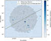 |
Fig. 1 Distribution of the dynamic spectra directions (beams) within our observing FoV, overlaid on a NenuFAR broadband (30–78 MHz) Stokes I image of background astronomical radio sources. Each gray circle corresponds to a direction for the synthesized IQUV dynamic spectra. The dashed line represents the predicted path of STARLINK3647 across the FoV from 16:19:57 to 16:20:31 on 6 June 2024, calculated using TLE data. |
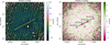 |
Fig. 2 Stokes I and Stokes V images produced with NenuFAR data, illustrating STARLINK-31034 passing through the FoV. The images were created using data collected between 54 and 66 MHz on 6 June 2024, between 16:29:46 and 16:29:57. The black circles overlaid on the Stokes V image represent the predicted positions of the Starlink satellite, calculated using TLE data. The corresponding times for each position are annotated next to the circles. They illustrate the satellite motion. |
4 Results
Over the course of 40 hours of observations, we detected radio signals from 134 Starlink satellite passes. These detections were largely from satellites that were not our primary targets. Among the targeted observations, STARLINK-31034 and the ISS were detected, while STARLINK-3647 and STARLINK-3657 were not. We note that 5 hours of data were excluded from the analysis due to adverse weather conditions and temporary instrumental issues. This resulted in an effective detection rate of approximately one satellite pass every 15 minutes for a field with a size of 20 degrees. A comprehensive summary of these detections is provided in Table A.1, including details such as the passing time, flux density, and peak emission frequency.
An example of a detected satellite pass is shown in Figure 2, which highlights the trail left by STARLINK-31034 as it crossed the NenuFAR FoV. Clear trails are visible in the Stokes I and V images. The predicted positions of the satellite, calculated using TLE data, are overlaid on the Stokes V image as black circles, and the observed satellite trajectory closely aligns with these predictions. Both images were generated using visibilities within the 54–66 MHz frequency range, corresponding to the peak of the broadband spectra of the satellites (see Section 4.1). The data were integrated over a 15-second window around the time of detection, which matches the estimated passage duration of the satellite.
Within the two image panels, the signal-to-noise ratio (S/N) is significantly higher in the Stokes V image, indicating that the satellite emission is strongly polarized (see Section 4.2). The high S/N is also caused by the lower noise levels in Stokes V (0.65 Jy/beam), as the sky background is predominantly unpolarized at low frequencies. In contrast, the Stokes I image displays a higher overall noise level (3.2 Jy/beam) due to confusion noise and the PSF sidelobe, together with bright points that correspond to background astronomical radio sources.
4.1 Continuum spectra
Visual inspection of the dynamic spectra revealed that Starlink satellite emissions are primarily concentrated between 54 and 66 MHz. Consequently, the flux density of the detected emissions was calculated by integrating over this frequency range (see Table A.1).
Based on this definition, the flux density of the detected satellite passes ranges from a few Jy to several hundred Jy. Notably, the brighter passes (>100 Jy) exhibit a consistent pattern in their broadband Stokes I spectra: The satellite emissions are detectable within the broader range of 33–73 MHz, with a distinctive double-peak structure that is clearly visible between 54 and 66 MHz, as shown in Figure 3. In this figure, each channel represents a 97.5 kHz frequency bin, and the signal and noise were calculated by stacking multiple dynamic spectra along the satellite trajectory to enhance the S/N.
The actual flux density6 is expected to be higher than the apparent flux density shown in Figure 3 due to two key factors: (1) the apparent flux density was used to ensure a consistent noise level across the satellite path for stacking purposes, while the actual flux density would be higher after applying primary beam correction; and (2) the flux density estimate was based on dynamic spectra generated for fixed pointings while the satellite moved through the beams. This resulted in an averaged measurement.
A particularly concerning observation is the detection of satellite emissions within frequency bands that are specifically protected for radio astronomy, as defined in the Radio Regulations7 published by the Radiocommunication Sector of the International Telecommunication Union (ITU-R). Two such protected bands fall within our observational range: 37.5–38.25 MHz (continuum observations), and 73–74.6 MHz (solar wind observations and continuum observations). For the STARLINK-31034 pass, no significant emission was detected in the first protected band, but the flux density exceeded 5σ between 73.29 and 73.39 MHz within the second band, with an additional tentative detection of 3.9σ between 73.39 and 73.48 MHz. This confirms that Starlink satellites are capable of producing detectable emissions within frequency ranges that are explicitly allocated to radio astronomy. However, these emissions are weak and only affect a limited region of the sky for a brief duration during each satellite pass.
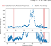 |
Fig. 3 Broadband Stokes I spectrum for STARLINK-31034, stacked along its trajectory across the NenuFAR FoV. The top panel shows the apparent flux density across the full NenuFAR observing frequency range, and the bottom panel provides a zoomed-in view in which the apparent flux density ranges from 0 to 50 Jy to highlight details of the spectrum outside the peak frequencies. In both panels, the radio-astronomy-protected frequency bands (37.5–38.25 MHz and 73–74.6 MHz) are shaded in red. |
4.2 Polarized spectra
Unlike the consistency observed in total intensity, the polarization properties of the detected emissions vary significantly across satellite passes. For each pass, the polarization spectrum exhibits fluctuations as the satellite moves through the FoV. This variability is likely influenced by the satellite-telescope geometry: Polarization depends inherently on the direction, and the relative positioning of the satellite and telescope may affect the observed polarization characteristics.
Despite this variability, a notable feature common to all detected satellite passes is the high degree of fractional polarization, as illustrated in Table A.1. Figure 4 shows full-Stokes spectra from a satellite path near the zenith. For this analysis, we used the IQUV dynamic spectra collected when the satellite was closest to the phase center. The analysis of these spectra indicates that the broadband emission was approximately 90% polarized, comprising 68% circular polarization and 22% linear polarization8.
In the linear polarization spectra, evidence of the Faraday effect was observed. The Stokes Q and U spectra displayed sinusoidal patterns consistent with Faraday rotation. To quantify this effect, we performed a rotation measure (RM) synthesis (Brentjens & de Bruyn 2005) on the Stokes Q and U spectra and compared the resulting Faraday dispersion function (FDF) with ionospheric RM measurements derived from GPS data (Mevius 2018). The FDF revealed multiple peaks, including one near RM = 0 and others at nonzero RM values. The peak near zero RM is likely due to residual instrumental polarization (leakage), a known issue in low-frequency polarimetric imaging. The additional RM components suggest, however, that the emission mechanism may not be stable. This might indicate malfunctions or unintended behaviors within the satellite onboard systems.
5 Discussion
The detection of radio emissions from Starlink satellites raises several questions about the nature of these signals and their implications for low-frequency radio astronomy. It remains to be determined whether these emissions are the result of direct satellite transmissions, reflections of astronomical or terrestrial signals, or unintended intrinsic emissions from the satellites themselves. The physical mechanisms that might underlie their observed frequency, polarization, and variability need to be clarified as well.
Beyond their origin, these signals prompt concerns about their impact on various areas of radio astronomy, including transient searches and nontransient studies such as spectroscopic and continuum surveys and cosmic magnetism. With the rapid expansion of satellite mega-constellations, we need to define strategies that can be developed to mitigate their influence and to ensure the quality of astronomical data.
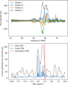 |
Fig. 4 Polarized spectra for STARLINK-31034, obtained from a single beam near the center of the FoV. The top panel displays the Stokes IQUV spectra of the satellite, and the bottom panel shows the result of the RM synthesis on the linear polarization. The vertical red line in the bottom panel indicates the ionospheric RM at the time the IQUV spectra were collected, as estimated using GPS data. |
5.1 Origin of the detected emission from Starlink
Based on the constraints of international frequency allocations, it is improbable that the detected signals represent direct, intentional emissions from Starlink satellites. Starlink satellites primarily operate in higher-frequency bands that are allocated for satellite communication, including the Ku-band (10.7–12.7 GHz and 14.0–14.5 GHz), Ka-band (17.7− 20.2 GHz and 27.5–30.0 GHz), V-band (37.5–51.4 GHz), and E-band (71.0–76.0 GHz and 81.0–86.0 GHz), which are used for the data transmission and reception with ground stations and users. These operational frequencies, authorized by the Federal Communications Commission (FCC), are significantly higher than the 60 MHz range in which our detections were made9.
This observation narrows the potential origins of the detected emissions to two main hypotheses: Either the signals are reflections of radio signals by the satellites, or they are unintended emissions generated by the satellites themselves.
5.1.1 Reflection of radio signals
If the detected signals were reflections from Starlink satellites, one potential origin might be solar radio emission. Solar activities are known to exhibit strong circular polarization at low frequencies (Sasikumar Raja & Ramesh 2013; McCauley et al. 2019). Our observations were conducted in June and July 2024, during a period approaching the solar maximum10 of the 11-year cycle, when increased solar activity was expected.
To test this hypothesis, we performed several nighttime observations, assuming that the satellites would be in Earth’s shadow and shielded from solar radio emission. Multiple detections were made at night. However, detailed calculations using TLE data revealed that all Starlink passes observed during our nighttime sessions were illuminated by the Sun, including the passes that were not detected. This was due to the timing of our observations near the summer solstice, when the Sun’s elevation at the NenuFAR site (latitude +47 degrees) remained above approximately −23 degrees even at midnight. Because of the satellite altitudes of several hundred kilometers above Earth’s surface, they remained illuminated by the Sun throughout day and night11. Consequently, our nighttime detections could not conclusively rule out solar emission as a potential source.
Despite this, the broadband structure of the detected signals, particularly the distinct peak around 60 MHz, does not align with the characteristics of typical solar radio bursts, which generally exhibit frequency drifts or broad continuous frequency ranges without distinct peaks (Zucca et al. 2012; White 2024). These discrepancies strongly suggest that the detected signals are not direct reflections of solar emission. However, preliminary results from LBA all-sky imaging with the LOFAR2.0 test stations (Bassa et al., in prep.) and early findings from NenuFAR exoplanetary observations (Zhang et al., in prep.) indicate that the Starlink satellites appear fainter or undetectable when they are in Earth’s shadow. This suggests a possible link between the emissions and the power generation via solar panels. Further dedicated studies are needed to confirm this correlation.
We also considered the possibility that the detected signals might be reflections of other bright celestial radio sources, particularly the Galactic plane and strong radio sources such as Cygnus A and Cassiopeia A. These sources are among the brightest in the radio sky and emit strongly across a broad range of frequencies, and their reflections have been proposed as a potential origin for low-frequency radio emissions associated with meteors (Dijkema et al. 2021). However, the Galactic plane and these bright sources are both effectively unpolarized at low frequencies. Their synchrotron radiation, which is inherently dominated by linear polarization, undergoes significant depolarization due to Faraday effects (Beck et al. 2013). Thus, the significant circular polarization exhibited in Starlink detections is inconsistent with the expected polarization characteristics of these sources. Furthermore, the distinctive peak structure of the detected signals does not align with the emission spectra of either the Galactic plane, Cygnus A, or Cassiopeia A. This further disfavors this hypothesis.
Another possibility we considered is that the detected emissions from Starlink satellites might be reflections of terrestrial signals because ground-based transmitters can produce strong signals within various frequency ranges. For example, television broadcasts in Europe are allocated near 60 MHz and are predominantly linearly polarized, as noted in the European Table of Frequency Allocations and Applications12. However, the detected emissions from the Starlink satellites exhibit significant circular polarization, which is uncommon for terrestrial transmitters at these frequencies. This disparity in polarization characteristics makes it unlikely that the observed signals originate as reflections of terrestrial broadcasts.
To further test the hypothesis that the detected emissions were reflections of terrestrial signals, we compared the detections from the Starlink satellites with observations of other objects capable of reflecting ground-based signals: the International Space Station (ISS), and an Airbus A319 aircraft. The ISS and aircraft are both significantly larger and closer to Earth’s surface than the Starlink satellites (The size and altitude information for STARLINK-31097, the ISS, and an Airbus A319 were obtained from online sources13, 14, 15.). According to the radar equation (Skolnik 1980),

where Pr is the received power, Pt is the transmitted power, Gt and Gr are the gains of the transmitting and receiving antennas, σ is the radar cross-section of the reflecting object, λ is the wavelength, and R is the distance between the transmitter and the reflecting object. This equation indicates that larger and closer objects should produce stronger reflected signals.
If the Starlink detections were reflections of terrestrial signals, we would expect even stronger reflections from the ISS and aircraft because they are larger and lie closer. Specifically, reflections from the ISS are estimated to be 186.7 times stronger than those from the Starlink satellites, and aircraft reflections are estimated to be approximately 1.5 × 10⁸ times brighter16.
Our observations did not detect any signals from the ISS or the aircraft at 60 MHz17, however, as shown in Figure 5. This result strongly suggests that the detected emissions from the Starlink satellites are not simple reflections of terrestrial signals.
Finally, we evaluated the power requirements for a hypothetical transmitter under the assumption that the detected signals result from reflections. Our observations revealed broadband emission exceeding 200 Jy from STARLINK-31034 over the 54–66 MHz range at an altitude of 440 km. Because each solar panel measures 15 × 4 m, we assumed an ideal effective reflecting area of 120 m2 for two panels. Consequently, the radar equation yields two scenarios:
If the transmitter were astronomical, it would need to emit more than 4 × 10¹² Jy in this frequency range. This flux density far exceeds even the most active solar bursts (White et al. 2023);
If the transmitter were based on the ground, its required power output would exceed 1.2 MW, which is substantially higher than that of most radio transmitters (e.g., TV broadcasters) operating in this frequency range.
Both cases present implausible conditions. This means that it is unlikely that the detected signals originate from simple reflections.
5.1.2 Unintended intrinsic emissions
We excluded direct emissions in the allocated frequency bands and reflections of external signals. We next considered the possibility that the detected signals arise from unintended intrinsic emissions within the satellite systems themselves. Satellites, particularly those in complex constellations such as Starlink, house sophisticated electronics, antennas, and power systems that may produce emissions outside their intended operational bands.
Unintended intrinsic emissions from satellites can originate from several sources, as outlined in studies of electromagnetic compatibility (EMC) in complex systems (Paul 1992). These emissions often arise from the nonlinear behavior of onboard electronic components, such as power-supply circuits, oscillators, and high-speed digital processors. The switch of noise from power supplies, particularly in systems using pulse-width modulation (PWM), can generate harmonics that propagate through the satellite structure. Similarly, high-speed digital circuits can produce transient electromagnetic fields due to rapid changes in current flow, leading to broad-spectrum emissions. Coupling between adjacent systems can exacerbate these effects by introducing additional resonances or feedback loops. The distinct peak observed around 60 MHz suggests the possibility of resonance effects within the satellite structure, potentially involving components such as solar panels acting as resonant elements at these frequencies. These complexities highlight the challenges of designing satellite systems that minimize these emissions while maintaining performance.
To explore whether the detected signals originate from unintended intrinsic emissions, we examined the detection rates and flux density levels across different generations of the Starlink satellites. The Starlink satellites can be broadly categorized into two primary versions: the earlier V0.9, V1.0, and V1.5 models, and the more recent V2-mini satellites. While both versions are designed to deliver broadband internet services, the V2-mini satellites introduce significant advancements. These include permission to operate at lower orbital altitudes, the addition of VHF beacon systems for telemetry, tracking, and command (TT&C) during orbit-raising and emergencies, and improvements in autonomous collision-avoidance systems18. By comparing detection rates and signal characteristics between these versions, we aimed to assess how changes in satellite hardware might influence the properties of unintended emissions, providing valuable insights into their origins. A recent LOFAR study by Bassa et al. (2024) highlighted significant differences in emissions between the two Starlink generations, and it reinforced the potential impact of hardware configurations on these signals.
Based on these considerations, we analyzed the statistics of the older and newer Starlink satellites, as illustrated in Figure 6. The figure presents the flux density and detection rates of the Starlink satellites as a function of their NORAD19 IDs (a unique identifier assigned to each artificial satellite). NORAD IDs are assigned sequentially, and earlier IDs correspond to satellites launched earlier in time.
Our observations reveal a striking contrast between the two versions of Starlink satellites. Nearly all passes of the newer V2mini satellites were detected within the NenuFAR observational FoV, and the flux density levels frequently surpassed those of the older versions and reached a few hundred Jy. In comparison, the older satellites yielded detectable signals during only a few percent of the total passes, and all detections exhibited flux density levels below 50 Jy.
The reflective properties of the two satellite generations should be similar, and the stark difference in the detection rates and flux density levels therefore argues against the reflection hypothesis as the primary cause of the observed signals. Instead, the upgraded systems on the V2-mini satellites may cause their increased detectability. These emissions are likely unintended and incidental and arise as byproducts of the new hardware configurations or enhanced power systems.
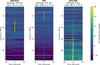 |
Fig. 5 Dynamic spectra of three objects observed with NenuFAR: STARLINK-31097, the International Space Station (ISS), and an Airbus A319 aircraft. The x-axis represents time, with 0 seconds corresponding to the time of the target detection. The altitudes of the objects, determined at the time of detection, and their sizes (length times width) are listed in each panel. The noise level in the aircraft panel is higher than in the other two panels because the aircraft observation occurred during the daytime, while the Starlink and ISS observations were made at night. The gray shaded regions in each panel indicate frequency channels that are known to be contaminated by RFI. These were masked during the analysis. |
5.2 Impacts on radio astronomy
The increasing presence of Starlink satellites in orbit poses significant challenges to various aspects of radio astronomy. These challenges include technical issues during data calibration and disruptions in specific scientific fields. Thoughtful mitigation strategies are required to address them.
5.2.1 Technical challenges: Calibration and near-field effects
The transient and bright nature of Starlink satellites poses significant challenges to calibration in low-frequency interferometry, particularly self-calibration. These challenges become critical when the solution intervals of self-calibration are at the scale of a minute or smaller. This is comparable to the time it takes for a satellite to traverse the FoV. Self-calibration relies on accurate sky models that map the distribution of the flux density from known celestial sources. However, since the transient flux density from the Starlink satellites is difficult to incorporate into sky models, their presence introduces unmodeled signals in the observations. This leads to errors in the reconstructed flux densities of celestial sources.
These challenges are further amplified in advanced calibration methods, such as polarimetric calibration and direction-dependent calibration, because the number of sources that are included in the relevant sky models is limited. At gigahertz frequencies, polarized sources such as radio galaxies and pulsars are prominent, but at frequencies below 100 MHz, most of these sources are depolarized due to Faraday rotation across the observing bandwidth and spatial variations in polarization angle (Lenc et al. 2017). This means that very few celestial sources are intrinsically polarized at these frequencies. As a result, it is often assumed that all sources in the sky model are unpolarized to simplify the calibration process. However, the Starlink satellites exhibit significant polarization, making them dominant contributors to the observed polarized sky. In a full-Stokes calibration where the Q, U, and V components are fitted, the presence of polarized flux density from these satellites violates the unpolarized assumption and causes genuinely unpolarized sources in the sky model to appear artificially polarized. This generates spurious artifacts in the data.
Direction-dependent calibration introduces additional complications. In this method, the FoV is divided into smaller regions, each assigned its own calibration solution to account for spatially varying instrumental and ionospheric effects (Kazemi et al. 2011; Tasse et al. 2021). Although a single satellite pass may not dominate the total flux density across the entire FoV, its localized brightness can significantly affect the calibration of individual facets. This localized distortion can degrade the quality of calibration solutions across the FoV and reduces the overall fidelity of the reconstructed images.
In addition to these calibration challenges, another important consideration is the near-field nature of Starlink satellites.
While standard interferometric imaging assumes sources to be in the far field, satellites in LEO can violate this assumption, especially for arrays with long baselines. In the near field, wave-front curvature across the array becomes non-negligible and might lead to decorrelation and reduced calibration accuracy if not accounted for. Recent work has demonstrated near-field aperture synthesis techniques that restore coherence for LEO satellites (Prabu et al. 2023), as well as methods for correcting for near-field effects and estimating emitter altitudes using interferometric data (Ducharme & Pober 2025). These methods may become increasingly important as satellite constellations grow.
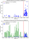 |
Fig. 6 Flux density and detection statistics of the Starlink satellites by NORAD ID. The top panel shows the Stokes I flux density of detected satellites, integrated over the 54–66 MHz range and one-second intervals. The vertical dashed line at NORAD ID 57457 (corresponding to STARLINK-30165) indicates the transition to the newer V2-mini Starlink satellites. The bottom panel presents histograms of the number of detections (blue) and total satellite passes (green) as a function of NORAD ID, highlighting the increased detectability of the V2-mini satellites. |
5.2.2 Scientific challenges: Transient and nontransient studies
Even with an accurate calibration, the presence of the Starlink satellites still impacts data products in various research fields.
For transient studies, including pulsars, fast radio bursts (FRBs), long-period transients (Hurley-Walker et al. 2022, 2023), exoplanets, and flare stars, the bright bursts introduced by the Starlink satellites into dynamic spectra complicate the identification of genuine astrophysical signals. These bursts require additional verification steps for candidate detections. One straightforward approach is imaging: The Starlink satellites move rapidly across the sky, with angular velocities of 1–2 degrees per second near the zenith20. By creating images with integration times of a few seconds, these satellites leave distinct trails that clearly indicate contamination, which can be removed via multidimension masking (Gehlot et al. 2024). Another method involves dispersion tests: Many astrophysical transients exhibit nonzero dispersion measures (DM) due to their propagation through the interstellar medium, whereas satelliteinduced bursts remain at DM = 0. Dispersion tests provide a reliable way to distinguish genuine astrophysical sources from satellite-induced signals. In this case, a compromise must be chosen from the point of view of ensuring a sufficiently wide frequency band, frequency and time resolution, and the proposed new criterion for distinguishing from satellite signals, the spatial criterion.
Nontransient studies, such as surveys, cosmic magnetism, and 21 cm cosmology research (Gehlot et al. 2024), face significant challenges from the presence of Starlink satellites. While emissions from individual satellites may average out in datasets that are stacked over multiple hours, the cumulative effect of numerous satellite trails21 introduces additional noise, which can be referred to as the satellite meterwave foreground. This added noise elevates the overall noise level in the final data products, potentially masking faint astrophysical signals and complicating foreground-removal techniques.
5.2.3 Potential mitigation strategies
Addressing the impact of the Starlink satellites on radio astronomy requires targeted mitigation strategies. A common approach involves multidimensional masking techniques (Gehlot et al. 2024) that filter transient RFI in the image domain. However, since satellite trajectories are predictable, a simpler approach is to cross-match observational data with predicted satellite passes and flag contaminated time segments. Both methods can effectively reduce satellite-induced noise, but they come at the cost of decreasing the amount of usable data. More advanced solutions are also being explored, such as the TABASCAL22 project (Finlay et al. 2023), which proposes adaptive calibration techniques capable of modeling moving satellite signals. The practical implementation remains extremely challenging, however.
As of July 2024, there are approximately 1000 V2-mini satellites in orbit23, which dominate the Starlink-related RFI below 100 MHz. For a wide-FoV array such as NenuFAR, excluding time segments when a V2-mini satellite is within the imaging FoV results in a loss of about 1.5% of the observational data24. This is an acceptable compromise for many studies. However, SpaceX plans to launch up to 29988 additional V2 satellites25. If similar emissions persist in future launches, the fraction of contaminated data could rise to approximately 45%. This significant data loss would severely hinder long-duration studies and would pose serious challenges to research in multiple fields of low-frequency radio astronomy, including experiments targeting the faint 21 cm signal from the early Universe (Wilensky et al. 2020). Moreover, this estimate only accounts for Starlink, while additional planned mega-constellations, such as the Amazon Project Kuiper26, could further exacerbate the impact.
Collaboration between the astronomical community and satellite operators is a necessary pathway to mitigate these challenges. Examples of such efforts include the SpaceX Darksat, which reduced the optical brightness by approximately 0.77 magnitudes (Tregloan-Reed et al. 2020), and the Green Bank Telescope (GBT) collaboration, where SpaceX implemented a boresight avoidance strategy to significantly reduce downlink RFI (Nhan et al. 2024). These initiatives highlight the potential of coordinated solutions, such as incorporating RFI mitigation into satellite design, developing predictive contamination models for satellites, and implementing operational protocols. Sustained collaboration is essential to ensure the future sustainability of low-frequency radio astronomy in the era of satellite mega-constellations.
6 Conclusions
We reported the detection and analysis of broadband radio emissions from Starlink satellites below 100 MHz using NenuFAR. Over 40 hours of observations, we identified 134 satellite passes, with flux densities ranging from 2 Jy to 261 Jy. The emission exhibited a broadband spectrum with distinctive features, including a double-peak structure between 54–66 MHz and significant circular polarization. Our analysis indicates that the detected signals are likely unintended intrinsic emissions from the satellites, associated with hardware configurations or onboard electronics, in particular, in the newer V2-mini satellites.
These detections present substantial challenges to radio astronomy. The transient and polarized nature of the emissions disrupts calibration processes, in particular, polarimetric and direction-dependent calibration, and it complicates transient searches by introducing false signals. Nontransient studies face increased noise levels from cumulative satellite trails, which could obscure faint astrophysical signals and reduce observational sensitivity. These issues are expected to worsen significantly with the planned expansion of satellite mega-constellations.
Mitigation strategies, including data flagging and exclusion of contaminated time segments, offer partial relief, but are insufficient in the long term. As the number of satellites increases, collaborative efforts between astronomers and satellite operators is crucial. Collaborative efforts between the astronomical community and satellite operators have shown promise, in particular, in addressing challenges in optical and radio astronomy. Future initiatives should focus on improving the satellite designs, refining operations, and developing tools for predicting and mitigating satellite contamination in radio observations.
Acknowledgements
The authors acknowledge funding from the ERC under the European Union’s Horizon 2020 research and innovation program (grant agreement no. 101020459 – Exoradio). This work is based on data obtained using the NenuFAR radiotelescope. NenuFAR has benefited from the funding from CNRS/INSU, Observatoire de Paris, Observatoire Radioastronomique de Nançay, Université d’Orléans, Région Centre-Val de Loire, DIM-ACAV -ACAV+ & -Origines de la Région Ile de France, and Agence Nationale de la Recherche. We acknowledge the collective work from the NenuFAR-France collaboration for making NenuFAR operational, and the Nançay Data Center resources used for data reduction and storage. X.Z. acknowledges the support of a postdoctoral fellowship at CSIRO, Australia, where the low-frequency polarimetry techniques developed during that time contributed to this work. X.Z. thanks L. Lamy for the insightful discussions on the potential origins of the detected signals. J.D.T. was supported for this work by the TESS Guest Investigator Program G06165 and by NASA through the NASA Hubble Fellowship grant #HST-HF2-51495.001-A awarded by the Space Telescope Science Institute, which is operated by the Association of Universities for Research in Astronomy, Incorporated, under NASA contract NAS5-26555. L.V.E.K. acknowledges the financial support from the European Research Council (ERC) under the European Union’s Horizon 2020 research and innovation program (Grant agreement no. 884760, “CoDEX”) The authors acknowledge the use of AI-assisted copy editing (ChatGPT) to improve the text of the manuscript.
Appendix A Summary of Starlink satellite detections with NenuFAR
Summary of Starlink satellite detections with NenuFAR.
References
- Bassa, C. G., Di Vruno, F., Winkel, B., et al. 2024, A&A, 689, L10 [Google Scholar]
- Beck, R., Anderson, J., Heald, G., et al. 2013, Astron. Nachr., 334, 548 [Google Scholar]
- Brentjens, M. A., & de Bruyn, A. G., 2005, A&A, 441, 1217 [NASA ADS] [CrossRef] [EDP Sciences] [Google Scholar]
- Dijkema, T. J., Bassa, C., Kuiack, M., et al. 2021, WGN, J. Int. Meteor Organ., 49, 137 [Google Scholar]
- Di Vruno, F., Winkel, B., Bassa, C. G., et al. 2023, A&A, 676, A75 [NASA ADS] [CrossRef] [EDP Sciences] [Google Scholar]
- Ducharme, J. M., & Pober, J. C., 2025, PASA, 42, e010 [Google Scholar]
- Finlay, C., Bassett, B. A., Kunz, M., & Oozeer, N., 2023, MNRAS, 524, 3231 [Google Scholar]
- Gallozzi, S., Scardia, M., & Maris, M., 2020, arXiv e-prints [arXiv:2001.10952] [Google Scholar]
- Gehlot, B. K., Koopmans, L. V. E., Brackenhoff, S. A., et al. 2024, A&A, 681, A71 [NASA ADS] [CrossRef] [EDP Sciences] [Google Scholar]
- Grießmeier, J.-M., Brionne, M., Kondratiev, V., et al. 2021, A&A, 652, A34 [NASA ADS] [CrossRef] [EDP Sciences] [Google Scholar]
- Grigg, D., Tingay, S. J., Sokolowski, M., et al. 2023, A&A, 678, L6 [NASA ADS] [CrossRef] [EDP Sciences] [Google Scholar]
- Grigg, D., Tingay, S., Prabu, S., Sokolowski, M., & Indermuehle, B., 2025, PASA, 42, e015 [CrossRef] [Google Scholar]
- Hainaut, O. R., & Williams, A. P., 2020, A&A, 636, A121 [EDP Sciences] [Google Scholar]
- Hurley-Walker, N., Zhang, X., Bahramian, A., et al. 2022, Nature, 601, 526 [NASA ADS] [CrossRef] [Google Scholar]
- Hurley-Walker, N., Rea, N., McSweeney, S. J., et al. 2023, Nature, 619, 487 [NASA ADS] [CrossRef] [Google Scholar]
- Kazemi, S., Yatawatta, S., Zaroubi, S., et al. 2011, MNRAS, 414, 1656 [Google Scholar]
- Kondratiev, V. I., Verbiest, J. P. W., Hessels, J. W. T., et al. 2016, A&A, 585, A128 [NASA ADS] [CrossRef] [EDP Sciences] [Google Scholar]
- Koopmans, L., Pritchard, J., Mellema, G., et al. 2015, in Advancing Astrophysics with the Square Kilometre Array (AASKA14), 1 [Google Scholar]
- Kruk, S., García-Martín, P., Popescu, M., et al. 2023, Nat. Astron., 7, 262 [CrossRef] [Google Scholar]
- Labate, M. G., Waterson, M., Alachkar, B., et al. 2022, J. Astron. Telesc. Instrum. Syst., 8, 011024 [NASA ADS] [CrossRef] [Google Scholar]
- Lazio, T. Joseph, W., Farrell, W. M., Dietrick, J., et al. 2004, ApJ, 612, 511 [Google Scholar]
- Lenc, E., Anderson, C. S., Barry, N., et al. 2017, PASA, 34, e040 [CrossRef] [Google Scholar]
- Loh, A., & the NenuFAR team 2020, https://doi.org/10.5281/zenodo.3667815 [Google Scholar]
- McCauley, P. I., Cairns, I. H., White, S. M., et al. 2019, Sol. Phys., 294, 106 [NASA ADS] [CrossRef] [Google Scholar]
- McDowell, J. C., 2020, ApJ, 892, L36 [Google Scholar]
- Mellema, G., Koopmans, L. V. E., Abdalla, F. A., et al. 2013, Exp. Astron., 36, 235 [NASA ADS] [CrossRef] [Google Scholar]
- Mevius, M., 2018, Astrophysics Source Code Library [record asc1:1806.024] [Google Scholar]
- Munshi, S., Mertens, F. G., Koopmans, L. V. E., et al. 2024, A&A, 681, A62 [NASA ADS] [CrossRef] [EDP Sciences] [Google Scholar]
- Nhan, B. D., De Pree, C. G., Iverson, M., et al. 2024, ApJ, 971, L49 [Google Scholar]
- Offringa, A. R., van de Gronde, J. J., & Roerdink, J. B. T. M., 2012, A&A, 539, A95 [NASA ADS] [CrossRef] [EDP Sciences] [Google Scholar]
- Offringa, A. R., McKinley, B., Hurley-Walker, et al. 2014, MNRAS, 444, 606 [NASA ADS] [CrossRef] [Google Scholar]
- Paul, C. R., 1992, Introduction to Electromagnetic Compatibility (New York: Wiley) [Google Scholar]
- Prabu, S., Hancock, P., Zhang, X., & Tingay, S. J., 2020, PASA, 37, e052 [Google Scholar]
- Prabu, S., Tingay, S. J., & Williams, A., 2023, PASA, 40, e056 [Google Scholar]
- Pritchard, J. R., & Loeb, A., 2012, Rep. Progr. Phys., 75, 086901 [CrossRef] [Google Scholar]
- Sasikumar Raja, K., & Ramesh, R., 2013, ApJ, 775, 38 [Google Scholar]
- Skolnik, M. I., 1980, Introduction to Radar Systems, 2nd edn. [Google Scholar]
- Stappers, B. W., Hessels, J. W. T., Alexov, A., et al. 2011, A&A, 530, A80 [NASA ADS] [CrossRef] [EDP Sciences] [Google Scholar]
- Tasse, C., 2023, killMS: Direction-dependent radio interferometric calibration package, Astrophysics Source Code Library [record ascl:2305.005] [Google Scholar]
- Tasse, C., Hugo, B., Mirmont, M., et al. 2018, A&A, 611, A87 [NASA ADS] [CrossRef] [EDP Sciences] [Google Scholar]
- Tasse, C., Shimwell, T., Hardcastle, M. J., et al. 2021, A&A, 648, A1 [EDP Sciences] [Google Scholar]
- Tasse, C., Hardcastle, M., Zarka, P., et al. 2025, Nat. Astron., submitted [Google Scholar]
- Toh, B. Y., Cahill, R., & Fusco, V. F., 2003, IEEE Trans. Educ., 46, 313 [Google Scholar]
- Tregloan-Reed, J., Otarola, A., Ortiz, E., et al. 2020, A&A, 637, L1 [EDP Sciences] [Google Scholar]
- Vallado, D. A., & Cefola, P. J., 2012, in 63rd International Astronautical Congress, Naples, Italy, 1 [Google Scholar]
- van Diepen, G., Dijkema, T. J., & Offringa, A., 2018, DPPP: Default Pre-Processing Pipeline, Astrophysics Source Code Library [record ascl:1804.003] [Google Scholar]
- van Haarlem, M. P., Wise, M. W., Gunst, A. W., et al. 2013, A&A, 556, A2 [NASA ADS] [CrossRef] [EDP Sciences] [Google Scholar]
- Walker, C., Hall, J., Allen, L., et al. 2020, in Bulletin of the American Astronomical Society, 52, 0206 [Google Scholar]
- Wayth, R., Sokolowski, M., Broderick, J., et al. 2022, J. Astron. Telesc. Instrum. Syst., 8, 011010 [Google Scholar]
- White, S. M., 2024, arXiv e-prints [arXiv:2405.00959] [Google Scholar]
- White, S., Yu, S., Chen, B., et al. 2023, in Bulletin of the American Astronomical Society, 55, 429 [Google Scholar]
- Wildemeersch, M., & Fortuny-Guasch, J., 2010, EC Joint Research Centre, Security Tech. Assessment Unit, Tech. Rep, 50 [Google Scholar]
- Wilensky, M. J., Barry, N., Morales, M. F., Hazelton, B. J., & Byrne, R., 2020, MNRAS, 498, 265 [CrossRef] [Google Scholar]
- Zarka, P., 2024, arXiv e-prints [arXiv:2409.16038] [Google Scholar]
- Zarka, P., Girard, J. N., Tagger, M., & Denis, L., 2012, in SF2A-2012: Proceedings of the Annual meeting of the French Society of Astronomy and Astrophysics, eds. S. Boissier, P. de Laverny, N. Nardetto, R. Samadi, D. Valls-Gabaud, & H. Wozniak, 687 [Google Scholar]
- Zarka, P., Lazio, J., & Hallinan, G., 2015, in Advancing Astrophysics with the Square Kilometre Array (AASKA14), 120 [CrossRef] [Google Scholar]
- Zarka, P., Denis, L., Tagger, M., et al. 2020, in URSI GASS 2020 [Google Scholar]
- Zhang, X., Zarka, P., Girard, J. N., et al. 2025, A&A, submitted [arXiv:2506.07912] [Google Scholar]
- Zucca, P., Carley, E. P., McCauley, J., et al. 2012, Sol. Phys., 280, 591 [Google Scholar]
SKA-Low: Square Kilometre Array – Low Frequency instrument.
AARTFAAC: Amsterdam-ASTRON Radio Transients Facility and Analysis Center.
The TLE data were retrieved from https://www.space-track.org/ using a database query, with constraints on the epoch range to match the time span of our observations.
In radio interferometry, the apparent flux density refers to the measured signal before corrections for instrumental and observational effects are applied, whereas the actual flux density represents the intrinsic brightness of the source after necessary corrections are applied. In our case, the actual flux density was obtained after we applied the primary beam correction, which accounts for the varying sensitivity across the FoV of the telescope.
https://www.itu.int/pub/R-REG-RR, accessed January 2025.
Although full-Stokes calibration was performed, residual instrumental polarization (i.e., leakage between Stokes parameters) is still present in the NenuFAR images. However, these leakage effects are typically at the level of a few percent, thus significantly lower than the ∼90% polarization observed from Starlink satellites.
Details of the frequency allocations for Starlink satellites can be found in the FCC document DA-24-1193A1, available at https://docs.fcc.gov/public/attachments/DA-24-1193A1.pdf (accessed November 2024).
The Sun reached maximum phase in October 2024. https://science.nasa.gov/science-research/heliophysics/nasa-noaa-sun-reaches-maximum-phase-in-11-year-solar-cycle/
This scenario resembles the midnight sun phenomenon in polar regions.
https://efis.cept.org, accessed November 2024, CEPT/ERC Report 25.
In practice, due to the relatively low altitude of aircraft, these reflections would require a transmitter positioned close to its flight path.
Signals from the ISS and aircraft were detected at other frequencies. However, determining whether these emissions are intrinsic or reflections is beyond the scope of this paper.
Details can be found in the FCC document DA-24-1193A1, available at https://docs.fcc.gov/public/attachments/DA-24-1193A1.pdf (accessed November 2024).
NORAD: North American Aerospace Defense Command.
Calculated using relevant TLE data.
For example, the detection rate of Starlink trails is approximately one trail per 15 minutes of observation for NenuFAR, as discussed in Section 4.
TABASCAL: TrAjectory BAsed RFI Subtraction and CALibration.
The list of satellites is derived from Space-Track, https://www.space-track.org/
This estimate is based on the typical satellite passage duration of approximately 15 seconds per 15-minute observation window.
Details are provided in the FCC document DA-24-1193A1, available at https://docs.fcc.gov/public/attachments/DA-24-1193A1.pdf
All Tables
All Figures
|
Fig. 1 Distribution of the dynamic spectra directions (beams) within our observing FoV, overlaid on a NenuFAR broadband (30–78 MHz) Stokes I image of background astronomical radio sources. Each gray circle corresponds to a direction for the synthesized IQUV dynamic spectra. The dashed line represents the predicted path of STARLINK3647 across the FoV from 16:19:57 to 16:20:31 on 6 June 2024, calculated using TLE data. |
| In the text | |
|
Fig. 2 Stokes I and Stokes V images produced with NenuFAR data, illustrating STARLINK-31034 passing through the FoV. The images were created using data collected between 54 and 66 MHz on 6 June 2024, between 16:29:46 and 16:29:57. The black circles overlaid on the Stokes V image represent the predicted positions of the Starlink satellite, calculated using TLE data. The corresponding times for each position are annotated next to the circles. They illustrate the satellite motion. |
| In the text | |
|
Fig. 3 Broadband Stokes I spectrum for STARLINK-31034, stacked along its trajectory across the NenuFAR FoV. The top panel shows the apparent flux density across the full NenuFAR observing frequency range, and the bottom panel provides a zoomed-in view in which the apparent flux density ranges from 0 to 50 Jy to highlight details of the spectrum outside the peak frequencies. In both panels, the radio-astronomy-protected frequency bands (37.5–38.25 MHz and 73–74.6 MHz) are shaded in red. |
| In the text | |
|
Fig. 4 Polarized spectra for STARLINK-31034, obtained from a single beam near the center of the FoV. The top panel displays the Stokes IQUV spectra of the satellite, and the bottom panel shows the result of the RM synthesis on the linear polarization. The vertical red line in the bottom panel indicates the ionospheric RM at the time the IQUV spectra were collected, as estimated using GPS data. |
| In the text | |
|
Fig. 5 Dynamic spectra of three objects observed with NenuFAR: STARLINK-31097, the International Space Station (ISS), and an Airbus A319 aircraft. The x-axis represents time, with 0 seconds corresponding to the time of the target detection. The altitudes of the objects, determined at the time of detection, and their sizes (length times width) are listed in each panel. The noise level in the aircraft panel is higher than in the other two panels because the aircraft observation occurred during the daytime, while the Starlink and ISS observations were made at night. The gray shaded regions in each panel indicate frequency channels that are known to be contaminated by RFI. These were masked during the analysis. |
| In the text | |
|
Fig. 6 Flux density and detection statistics of the Starlink satellites by NORAD ID. The top panel shows the Stokes I flux density of detected satellites, integrated over the 54–66 MHz range and one-second intervals. The vertical dashed line at NORAD ID 57457 (corresponding to STARLINK-30165) indicates the transition to the newer V2-mini Starlink satellites. The bottom panel presents histograms of the number of detections (blue) and total satellite passes (green) as a function of NORAD ID, highlighting the increased detectability of the V2-mini satellites. |
| In the text | |
Current usage metrics show cumulative count of Article Views (full-text article views including HTML views, PDF and ePub downloads, according to the available data) and Abstracts Views on Vision4Press platform.
Data correspond to usage on the plateform after 2015. The current usage metrics is available 48-96 hours after online publication and is updated daily on week days.
Initial download of the metrics may take a while.