| Issue |
A&A
Volume 698, June 2025
|
|
|---|---|---|
| Article Number | A117 | |
| Number of page(s) | 16 | |
| Section | Planets, planetary systems, and small bodies | |
| DOI | https://doi.org/10.1051/0004-6361/202554124 | |
| Published online | 06 June 2025 | |
Monitoring of asteroids in cometary orbits and activated asteroids through archival images and new observations★
1
Departamento de Astronomía, Facultad de Ciencias, Universidad de la República,
Iguá 4225,
11400
Montevideo,
Uruguay
2
Observatório Nacional,
R. Gen. José Cristino 77 - São Cristóvão,
Rio de Janeiro,
RJ -
20921-400
Brazil
3
Laboratório Interinstitucional de e-Astronomia - LIneA,
Av. Pastor Martin Luther King Jr, 126,
Rio de Janeiro -
RJ -
20765-000
Brazil
4
Instituto de Astrofísica de Canarias, C/ Vía Láctea s/n,
38205
La Laguna, Tenerife,
Spain
5
Department of Physics, University of Michigan,
Ann Arbor,
MI48109,
USA
6
Astronomy Department, University of Washington,
Box 351580,
Seattle,
WA
98195,
USA
7
Department of Physics & Astronomy, University College London,
Gower Street,
London
WC1E 6BT,
UK
8
Institut de Física d’Altes Energies (IFAE), The Barcelona Institute of Science and Technology, Campus UAB,
08193
Bellaterra (Barcelona)
Spain
9
School of Mathematics and Physics, University of Queensland,
Brisbane,
QLD 4072,
Australia
10
Centro de Investigaciones Energéticas, Medioambientales y Tecnológicas,
Madrid,
Spain
11
Fermi National Accelerator Laboratory,
PO Box 500,
Batavia,
IL
60510,
USA
12
California Institute of Technology,
1200 East California Blvd, MC 249-17,
Pasadena,
CA
91125,
USA
13
Instituto de Fisica Teorica UAM/CSIC, Universidad Autonoma de Madrid,
28049
Madrid,
Spain
14
Institut d’Estudis Espacials de Catalunya (IEEC),
08034
Barcelona,
Spain
15
Institute of Cosmology and Gravitation, University of Portsmouth,
PO1 3FX,
UK
16
University Observatory, Faculty of Physics,
Ludwig-MaximiliansUniversität, Scheinerstr. 1,
81679
Munich,
Germany
17
Center for Astrophysical Surveys, National Center for Supercomputing Applications,
Urbana,
IL
61801,
USA
18
Santa Cruz Institute for Particle Physics,
Santa Cruz,
CA
95064,
USA
19
Center for Astrophysics | Harvard & Smithsonian,
Cambridge,
MA
02138,
USA
20
Australian Astronomical Optics, Macquarie University,
North Ryde,
NSW
2113,
Australia
21
Department of Physics and Astronomy, Texas A&M University, College Station,
TX
77843,
USA
22
LPSC Grenoble -
53, Avenue des Martyrs
38026
Grenoble,
France
23
Kavli Institute for Particle Astrophysics & Cosmology, Stanford University,
Stanford,
CA
94305,
USA
24
SLAC National Accelerator Laboratory,
Menlo Park,
CA
94025,
USA
25
Department of Physics, Northeastern University,
Boston,
MA
02115,
USA
26
Physics Department, Lancaster University,
Lancaster,
LA1 4YB,
UK
27
Computer Science and Mathematics Division, Oak Ridge National Laboratory,
Oak Ridge,
TN
37831,
USA
28
Department of Physics, University of Michigan,
Ann Arbor,
MI
48109,
USA
29
Department of Astronomy, University of California,
Berkeley,
CA
94720,
USA
30
Lawrence Berkeley National Laboratory,
1 Cyclotron Road,
Berkeley,
CA
94720,
USA
★★ Corresponding author.
Received:
13
February
2025
Accepted:
2
April
2025
Abstract
Context. Transitional objects are minor bodies that share some characteristics with asteroids and others with comets. These objects include asteroids in cometary orbits (ACOs), which behave dynamically like comets, but lack observed activity, while activated asteroids (AAs) follow typical asteroidal orbits, but have shown dust ejections.
Aims. The monitoring of a set of these objects carried out in 2015 and 2016 is continued using archival images from various observatories and new data from the IMPACTON telescope in Brazil.
Methods. Two techniques were applied to detect activity: (i) surface brightness profiles were compared with those of field stars to identify widening, and (ii) the magnitudes reported in the Minor Planet Center, combined with our observations, were reduced and analyzed to identify abrupt brightness increases as a function of heliocentric distance.
Results. We analyzed the surface brightness profiles of 133 ACOs and 7 AAs. To study the reduced magnitude, we obtained data from the 705 ACOs that were known at the time of the analysis. Together with the data from our previous work, our analysis covered 23% of the total known ACOs; 8 deviated slightly in the surface brightness profile, 6 brightened in the reduced magnitude, and one object is in common in both samples. A very low percentage of objects might show activity (4% of the sample with brightness profiles and <1% in the reduced magnitudes). These results would rule out a slow transition from active to inert. Regarding AAs, 4 showed activity, and 3 of them matched previously reported periods, while the data we analyzed for P/2015 X6 were obtained 19 days before the first existing activity report. The activity episodes of these objects are very restricted in time and do not always occur in the same region of the orbit.
Key words: comets: general / minor planets, asteroids: general
Based on observations obtained at the Observatório Astronômico do Sertão de Itaparica (OASI) of the Observatório Nacional, Brazil, the Dark Energy Survey (DES) database, the Very Large Telescope (VLT) of the European Southern Observatory (ESO) and the Instituto de Astrofísica de Canarias (IAC).
© The Authors 2025
 Open Access article, published by EDP Sciences, under the terms of the Creative Commons Attribution License (https://creativecommons.org/licenses/by/4.0), which permits unrestricted use, distribution, and reproduction in any medium, provided the original work is properly cited.
This article is published in open access under the Subscribe to Open model. This email address is being protected from spambots. You need JavaScript enabled to view it. to support open access publication.
1 Introduction
The study of asteroids and comets has always been especially relevant because they are the remnants of the formation of the Solar System, and their physical and chemical properties have remained practically unchanged since their origins. When we analyze them, we may also be able to determine the conditions required for our planetary system to form, and its subsequent evolution.
Asteroids are rocky objects with nonexistent or negligible volatile substances, and they appear as inert bodies, whose brightness variations are solely attributed to rotational factors. Comets have a substantial ice content on their surface and interior, observationally have a coma, and can show one or more tails. However, comets do not show activity during their entire orbit, but do so when they approach the Sun. Even then, the detection of a coma or tail is contingent upon the prevailing observability conditions and the sensitivity of the instruments used. This introduces the possibility that objects with very low activity go unnoticed by the instruments that perform the observation if the instruments are not sensitive enough.
Tisserand’s parameter (Kresak 1979) has been fundamental for the historical classification of objects into asteroids and comets. The parameter arises from the restricted three-body problem. From the Jacobi integral, we can derive the Tisserand parameter, given by Eq. (1), where ap is the semimajor axis of the planet in circular orbit around the Sun, and a, e, and i are the semimajor axis, eccentricity, and inclination of the particle, respectively,
![Mathematical equation: $\[T_p=\frac{a_p}{a}+2 \sqrt{\frac{a}{a_p}\left(1-e^2\right)} cos (i).\]$](/articles/aa/full_html/2025/06/aa54124-25/aa54124-25-eq1.png) (1)
(1)
A purely dynamic criterion is to consider asteroids as objects with TJup > 3 and comets as objects with TJup < 3. However, this simple criterion has been questioned, and further refinements are necessary to achieve a proper classification scheme between these populations (see, e.g., Tancredi 2014).
As increasingly more objects were discovered, the categories that were traditionally used to classify them began to be insufficient. We commonly speak of “transitional objects” to refer to objects that do not fully fit one of the traditional categories. Hsieh (2017) called them “continuum objects”, in relation to the fact that there is no clear line that distinguishes them. We analyze two populations of transitional objects and refer to them as asteroids in cometary orbits (ACOs) and activated asteroids (AAs). We follow the clasification scheme presented by Tancredi (2014).
An ACO is an object whose orbit has a moderate to high inclination and eccentricity, with a low relative encounter velocity with Jupiter. It therefore belongs to an unstable population, similar to the Jupiter-family comets (JFCs), whose dynamic lives are about 104–105 years (see, e.g., Alvarez-Candal & Roig 2005 and Di Sisto et al. 2009).
Several physical studies (albedo determination, spectrum analysis, etc.) of ACOs have been carried out in the past decade, such as the works of Alvarez-Candal (2013), Kim et al. (2014), Licandro et al. (2016), Licandro et al. (2018), Simion et al. (2020), and Geem et al. (2022). From these works, it can be deduced that a high percentage of the studied objects are observationally compatible with cometary nuclei; that is, their albedos, colors, and spectra are similar. Some dynamic studies have also been carried out, among which we highlight the work of Hsieh & Haghighipour (2016). They showed that some objects with initial JFC orbits can evolve into orbits of main-belt asteroids on relatively short timescales (<2 Myr), and vice versa. Ye et al. (2016) also carried out dynamical studies on a large set of ACOs in the population of near-Earth asteroids (NEAs). They reported a lower limit of 2% dormant comets in the nearEarth object (NEO) population. However, the results reported by different authors must be compared with caution because varying criteria may have been used to classify an object within the ACOs population.
Moreover, activity has been observed in bodies that do not follow cometary orbits. Objects in the main asteroid belt were assumed to be inactive for a long time because it was thought that any volatiles they might have had sublimated during their lifetime. This concept was challenged, however, by the discovery of objects that were at first known as main-belt comets and later as active asteroids (Elst et al. 1996, Hsieh et al. 2004, and Hsieh & Jewitt 2006). Since then, a few dozen of these objects have been discovered (Chandler et al. 2024).
We will use the term ‘activated’ in this paper to refer to objects that exhibit a dynamic behavior similar to that of asteroids (regardless of whether they belong to the main belt) and that showed one or several episodes of activation in the past, that is, a coma and/or tail, without analyzing the generation mechanisms of this activity. The term refers to the fact that the activity is sporadic and is activated by some mechanism. So far, there is no consensus in the literature on whether there is a prevailing activation mechanism, and several alternatives have been discussed (see, e.g., Jewitt & Hsieh 2024).
To better understand the nature of these objects, we monitored 42 ACOs and 3 AAs in 2015 and 2026 using the telescope of the project Iniciativa de Mapeamento e Pesquisa de Asteroides nas Cercanias da Terra no Observatório Nacional (IMPACTON) of the Observatório Astronômico do Sertão de Itaparica (OASI). We detected activity in one of the observed ACOs (P/2015 PD229), as well as the reactivation of two AAs (238 P and 288 P) (Martino et al. 2019). In 2019, the study of these objects was continued in order to expand the sample. To do this, we again worked with the IMPACTON telescope and with archive images from different databases and observatories. The objective of this work is to study the nature of the ACOs to determine whether they are dormant or extinct comets, or asteroids that escaped from the main belt and are currently in cometary orbits. To do this, we need to know the size of this population of objects and the number that are inactive or present at least low levels of activity. Meanwhile, studying AAs to determine activity and inactivity periods throughout their orbit can help us understand the activation mechanisms.
2 Observations
Images of ACOs and AAs were obtained from different instruments. Prior to this, we selected the set of ACOs to be studied based on the criterion developed by Tancredi (2014).
2.1 Selection of objects
We downloaded the asteroid database from the Minor Planet Center (MPC) and the comet database from the Jet Propulsion Laboratory (JPL) of NASA for updated orbital elements for the asteroids and comets. We only considered asteroids with precise orbital elements according to the uncertainty parameter U provided by the MPC. This parameter is an integer in the range from 0 to 9, where 0 indicates a very small uncertainty, and 9 extremely large uncertainty. Recently discovered objects usually have a very high U parameter that decreases as new observations are obtained and the orbits are improved. For our selection, we used a maximum of U = 2, which according to the MPC represents a longitude runoff error <19.6″ per decade. In this way, we ruled out asteroids whose orbital elements are considered of poor quality to avoid contaminating the sample with objects that might not in fact be ACOs. The uncertainty parameter tends to decrease over time, so that objects that were initially discarded because their uncertainty was too large may eventually fall within our criteria.
Next, Tancredi’s criterion was applied. This separates the comets into JFC, Halley-type orbits (HTO), comets in asteroidal orbits (CAO), and Centaur comets (CC). HTOs have TJup < 2 and a < aNep; JFCs have 2 < TJup < 3.05 and q < QJup; CAOs have TJup > 3.05 and q < QJup; and CCs have TJup > 2 and QJup < q < aUra (here, q is the object perihelion, QJup is Jupiter aphelion, and aUra is Uranus semimajor axis). The ACOs are separated into ACOs-Jupiter family (ACOs-JF), ACOs-Centaur (ACOs-Cen), and ACOs-Halley orbits (ACOs-Hal). ACOs-JF have 2 < TJup < 3.05 and q < QJup, they are not in a resonance, and their values of the minimum orbital intersection distance (MOID) with respect to the giant planets are low; ACOs-Cen have TJup > 2 and QJup < q < aUra; and ACOs-Hal have TJup < 2.
Finally, we numerically integrated the objects with the RADAU orbital element integrator (Everhart 1985) using orbital solutions from the MPC for asteroids and from JPL for comets (nominal orbits). The encounters of the objects with the giant planets were evaluated as well. When the ACO had no close encounters (less than 1 au) with any giant planet, it was removed from the list. After all these stages were completed, we generated tables with the data from selected ACOs1.
Table 1 shows the data of asteroids, asteroids with precise orbits, and asteroids with a Tisserand parameter with respect to Jupiter smaller than 3, with data taken in July 2021. The table also lists data of the objects that we obtained in the selection distinguished by type of ACO and type of comet. Although the number of asteroids with TJup < 3 is quite high, the number of ACOs is far lower when a strict dynamic criterion is applied. The sample of objects to be analyzed consists of all ACOs (705) and comets in asteroidal orbits (31). More than 17 000 asteroids with TJup < 3 were listed on the mentioned date, but only 705 of these meet the more stringent criteria established by Tancredi. These criteria ensure that the truly dynamical behavior of these objects is compatible with cometary dynamics.
Number of asteroids, ACOs, and comets.
2.2 Instruments
Images of ACOs and AAs were obtained from different instruments. An observation plan was designed in collaboration with the IMPACTON team of the OASI, Pernambuco, Brazil. The observatory is equipped with a 1 m telescope. The images were taken with Apogee CCD cameras, model Alta U42 and Alta U47, with an R-Cousins filter. The details of the available instrumentation and sky characterization were reported by Rondón et al. (2020). Observations were made between August 2019 and April 2021. Most of the objects were observed only once, although some could be observed in two consecutive months. No restrictions on the true anomaly of the object were considered, although priority was given to observations close to perihelion. In most cases, two sequences of 15 images per object were taken. Bias, flat, and dark images were obtained to perform the basic calibration.
Through a collaboration with the Instituto de Astrofísica de Canarias (IAC) in Spain, we worked with a set of images of objects that were observed with the IAC80 telescope and the Jacobus Kapteyn Telescope (JKT) in 2015 and 2016. The IAC80 is located at the Teide Observatory on Tenerife, and the JKT is located at the Roque de los Muchachos Observatory on La Palma. Most of the observations with the IAC telescopes were made with the R filter, except for a few cases in which it was observed with the clear filter. Observations were made in November and December 2015, and between July and October 2016. The ACOs present in the images were selected with the same dynamic criteria as ours. The images provided to us were processed on bias, dark, and flat, so no prior calibration was required.
In addition, we worked with archive images from the Very Large Telescope (VLT), a group of European telescopes belonging to the European Southern Observatory (ESO) at Cerro Paranal, Chile. These images were obtained with the Unit Telescopes (8.2 meters), with the instrument FOcal Reducer and low dispersion Spectrograph (FORS) (Appenzeller et al. 1998). We accessed the VLT images using two online tools: Mega Precovery (MP; Vaduvescu et al. 2013) and Solar System Object Image Search (SSOIS; Gwyn et al. 2012). We obtained images in the filters V, R, and I. The images corresponded to different projects that observed these objects of interest, including Romon-Martin et al. (2002), Doressoundiram et al. (2005), Lorin & Rousselot (2007), DeMeo et al. (2008), Belskaya et al. (2010), and Tozzi et al. (2012). For most of the objects, no associated publications were found.
Finally, we used images from the Dark Energy Survey (DES), which is an international collaborative project that observed the sky over six years since 2013 and covered an area of 5000 square degrees of the celestial southern hemisphere. Observations were made in filters grizY. The instrument that was used is an extremely sensitive 570-megapixel digital camera, the Dark Energy Camera (DECam; see Flaugher et al. 2015), and it is located on the 4-meter Blanco telescope of the Cerro Tololo Inter-American Observatory. A total of 3374 images containing the coordinates of 195 different objects were obtained. In this archival search, the selection was not based on the predicted apparent magnitude of the objects. This led to cases in which the objects that were nominally within the instrument field of view were too faint to be recovered in the images. There were also no restrictions regarding the true anomaly of objects.
3 Data reduction
Two methods were used to detect activity on the objects: an analysis of the surface brightness profiles, and deviations in the reduced magnitude along the orbit.
3.1 Surface brightness profiles
Following the method described by Luu (1992), we applied the approach used previously by Martino et al. (2019). This technique involves comparing the surface brightness profiles of asteroids with those of stars. A widened profile indicates the existence of a cometary coma, and a profile similar to the stellar one corresponds to an object without activity.
All images were processed trough Python and Matlab scripts. The usual calibration was performed, along with the removal of bad pixels and cosmic rays. A plate solution was performed using Astrometry.net routines2. If there were image sequences, these were aligned on the stars and on the object, and the aligned images were added to increase the signal-to-noise ratio (S/N). The position of the object in the image was automatically calculated using JPL ephemerides.
The radial surface brightness profile of the object was obtained by fitting a Moffat function to the flux values as a function of the distance to the centroid. The same procedure was employed with a set of stars, and we obtained an average profile. Both profiles were plotted superimposed, and a visual inspection was performed with each plot in search of deviations.
Some of the archival images we obtained had long exposure times (more than 90 seconds), and in some cases, this caused an object to appear in the image as a trail. It was therefore not possible to obtain a radial profile. For these cases, we obtained the displacement values in right ascension and declination, and we rotated the image so that the trail remained horizontal in the image (this technique is more similar to the original proposed by Luu 1992). The average of the flux by rows was calculated, and then, we obtained the value of the centroid to plot the profiles.
3.2 Reduced magnitudes
The reduced magnitude is the magnitude that an object would have at a heliocentric distance r = 1 au, a geocentric distance Δ = 1 au, and a phase angle α = 0o (the absolute magnitude for a Solar System object is obtained from averaging several measurements of its reduced magnitude). For an inactive object (a bare nucleus), the reduced magnitude is expected to vary according to the rotational light curve. The rotation of the object generates a maximum amplitude in magnitude (Amax) according to Eq. (2), where a and b are the axes of the object. For example, a 1:5 axis ratio would generate a maximum amplitude of 1.75 magnitudes,
![Mathematical equation: $\[A_{max}=2.5 \log \frac{a}{b}.\]$](/articles/aa/full_html/2025/06/aa54124-25/aa54124-25-eq2.png) (2)
(2)
The study of the reduced magnitude versus the heliocentric distance enables us to find changes in brightness along the orbit of the objects, which serve as indicators of cometary activity. When an object is active, its brightness increases and its reduced magnitude decreases. It is therefore useful to detect these changes in brightness to generate plots of the reduced magnitude as a function of heliocentric distance with the available photometric data.
We used magnitude reports from different observers that are available in the MPC database. The limitations of this dataset were discussed in Martino et al. (2019), but the conclusion was that these observations provide a feasible approach to monitoring the object at various points in its orbit. This cannot be achieved by a single observer. Additionally, magnitudes computed from the data obtained from the different telescopes were added to the data. The apparent magnitudes were reduced by geocentric and heliocentric distance, as well as by phase angle, with a phase coefficient β = 0.04 mag/deg, according to Jewitt & Luu (1989) (Eqs. (3) and (4)) and were also transformed to a common band V by applying color corrections of a solar-like spectrum,
![Mathematical equation: $\[m(1,1, \alpha)=m(r, \Delta, \alpha)-5 \log (r \Delta)\]$](/articles/aa/full_html/2025/06/aa54124-25/aa54124-25-eq3.png) (3)
(3)
![Mathematical equation: $\[m(1,1,0)=m(1,1, \alpha)-\beta \alpha.\]$](/articles/aa/full_html/2025/06/aa54124-25/aa54124-25-eq4.png) (4)
(4)
The values of the reduced magnitude were plotted as a function of the heliocentric distance. All MPC data were used when their ephemerides matched those of the object at the time of observation. Data belonging to large surveys were highlighted in the plot. Then, we searched for significant differences between the calculated magnitudes and the reported average that could not be explained by other factors. We specifically searched for cases with more than one report of brightening, corresponding to different nights of observation and/or observers.
4 Results
The results of the profiles are presented in Sect. 4.1, and those of the reduced magnitudes are described in Sect. 4.2.
Summary of the profiles.
Summary of the objects by instrument.
4.1 Surface brightness profiles
A total of 413 surface brightness profiles of 140 studied objects were obtained because many of the objects were observed on different dates, and we therefore obtained several profiles per object. Table 2 shows the number of ACOs and AAs with a well-defined surface brightness profile, and their quality. The quality depends on the observation conditions and S/N of the object. The following values were adopted to define it, following Martino et al. (2019): A profile was considered to be of high quality when the mean deviation of the flux values did not exceed 5% of the normalized flux. A medium quality ranged between 5 and 10%, and a low quality meant that it exceeded 10%. To calculate the mean deviation, we selected a range of pixels (measured from the centroid of the object), typically between 4 and 8. These values were adjusted according to the night seeing. An object was considered to have high quality when at least one profile had this quality. The quality was considered to be medium when the best profile had this quality, and the quality was considered to be low when the profiles only had this quality. When the object appeared as a trail in the image, no quality calculations were made because only a few intensity values were available to make an adjustment. These objects appear in Table 2 as “Trails”. Although the data quality differs mainly depending on the brightness of the object, inactive objects are expected to present a similar profile to that of stars, regardless of the data dispersion.
Table 3 shows the number of ACOs and AAs with at least one profile, sorted by instrument (the totals consider objects without repetitions). The details of each observation can be found in Appendix A.
All brightness profiles were inspected for deviations from a stellar profile. For objects 29981, 54598, 90572, 515718, and 2015 BK22, at least one deviating profile was obtained. This might be an indication of slight cometary activity (Figs. 1a, b, c, d, and e, respectively). For C/2014 OG392 (PANSTARRS), we obtained a profile with a considerable widening, but with a high dispersion (Fig. 1f). This object has already been classified as a comet. The activity was discovered in archival images from July and August 2017, and it was confirmed with observations from August 2019 (Chandler et al. 2020). Our data corresponded to November 2018, which is between the two existing activity reports, and they were obtained from the DES project. Object 2016 YB13 appeared in the DES images as a trail. We obtained the profile shown in Fig. 1g, where the intensity values of the object appear to be clearly separated from the star profile.
Widened profiles were also obtained for three AAs: 259P, 311P, and P/2015 X6 (Figs. 1h, i, and j). In all cases, the activity was verified. For 259 P and 311 P, this is consistent with existing reports. In the first case, activity was present in DES images from September 2017, when it reactivated (Hsieh et al. 2017). Object 311P was also in DES images from September 2013. In this month, the first reports of activity (Bolin et al. 2013) were obtained. P/2015 X6 showed a widened profile in DES images from November 18, 2015, and the first activity for this object was reported on December 7, 2015 (Tubbiolo et al. 2015). Finally, 133P was present in images from July 2007 during its second activity episode. However, the profiles were not visibly widened. This outcome agrees with the findings of Hsieh et al. (2010), who studied the reactivation of the object. Their analysis revealed that while the object exhibited activity, the full width at half maximum (FWHM) of its brightness profile matched that of a stellar FWHM during those observations. This suggests that the object either lacked a coma or had an extremely compact one (smaller than 1″, corresponding to a linear diameter of 1200 km).
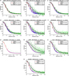 |
Fig. 1 Surface brightness profiles of (a) 29981 (VLT), (b) 54598 (IMPACTON), (c) 90572 (IMPACTON), (d) 515718 (DES), (e) 2015 BK22 (IMPACTON), (f) 2014 OG392 (DES), (g) 2016 YB13 (DES), (h) 259 P (DES), (i) 311 P (DES), and (j) P/2015 X6 (DES). The plots show the normalized intensity values of each pixel from the centroid for one or more stars (blue dots), the Moffat fit of the stars (red line), the normalized intensity values of the object (green dots), and the Moffat fit of the object (black line). The red error bars correspond to the stars and the black error bars to the object. The errors were calculated from the dispersion of the flux values with respect to the fit. A small artificial horizontal offset has been introduced in the position of the bars to avoid overlap. In the image header we list the object name, date, image range (when a set of images was coadded), image number or time, and the calculated magnitude. When the object appeared as a trail (2016 YB13), the intensity values of the trail are plotted superimposed with the profile of the stars (with their Moffat fit). |
4.2 Reduced magnitude
We created plots of the reduced magnitude as a function of the heliocentric distance for the 705 ACOs in the list and for the 7 AAs observed during this work, in which we included all the data from photometric observations reported to the MPC. The magnitudes calculated from the images we analyzed were also added to the data. The reduced magnitude plots of all the ACOs in our list were reviewed, and those with more than one report with brightening in the MPC data were separated. A summary analysis of these cases is presented below.
Objects 322966, 323137, and 2009 KF37 (Figs. 2c) differed from the absolute magnitude H. We were unable to attribute this to object rotation. The reports for 322966 correspond to a single observer and there are no other reports for the same dates, while two reports were made for 2009 KF37 from different observatories in different years. Object 323137 has already been classified as a comet (282P). This object belongs to the outer belt, and its Tisserand parameter is TJ = 2.99. It was observed to be active in 2013 and was found to also have activity in images taken in March 2012 (Bolin et al. 2013). The plots of the reduced magnitude show three brightening peaks with respect to the average magnitude, which correspond to reports made in 2001 (first observations of the object), 2003, and 2004. In particular, in July 2004, observers reported magnitudes between 12.54 and 13.14, and the absolute magnitude of the object is H = 15.3. Objects 275618 and 2017 QO33 (Figs. 2d and e) were present in several MPC reports in which a magnitude with an increased brightness was obtained. The reports corresponded to a single observatory, however, and other observers reported magnitudes close to the mean for the same dates.
On the other hand, we reviewed the plots in which the observations made during this work were included (our data appear in the plots as red squares). Three cases differ from the absolute magnitude of the MPC, considering the error in calculated magnitude: 54598, 2000 CN152, and 2014 SS303 (Figs. 2f, g, and h). Only object 54598 also showed a widened profile. The case of 2000 CN152 was discarded because the object was at the edge of the image, which may have caused a distortion in the flux values.
5 Discussion
We first discuss the results for the ACOs. Based on the criteria employed in this study, there are a total of 705 of these objects. We obtained surface brightness profiles of 133 ACOs and generated a cumulative total of 160 (considering our previous work). A total of 92 of these were identified as ACOs-JF, 50 as ACOs-Cen, and 18 as ACOs-Hal. Figure 3 shows the histograms of the heliocentric distance (r) of the objects at the time of observation. The data are categorized based on the heliocentric distances, specifically distinguishing between those at a distance smaller than and larger than 5 au.
We employed two activity indicators: (i) deviations in the brightness profile relative to the stellar profile, and (ii) a significant decrease in the reduced magnitude of the object.
The deviations of 7 of the 133 ACOs for which profiles were obtained cannot be attributed to external factors such as observability conditions or low S/N. These ACOs are 29981, 54598, 90572, 515718, C/2014 OG 392 (PANSTARRS), 2015 BK22, and 2016 YB13. One of these asteroids has already been classified as a comet. Moreover, a similar case of activity was previously documented for one of the objects we investigated in our prior study, that is, for the object that was originally classified as an asteroid and then as comet P/2015 PD229 ISON-Cameron (Martino et al. 2019). We found possible signs of activity for 8 of the 160 ACOs based on the surface profiles (5%).
By examining the reduced magnitude, we identified five objects with noteworthy deviations: 54598, 322966, 323137, 2009 KF37, and 2014 SS303. One of these objects is also officially classified as a comet: 282P (323137). In our previous study, only one ACO varied significantly in its reduced magnitude: 174P/(60558) Echeclus, which was also already classified as an asteroid and a comet. We found possible activity based on the reduced magnitudes for 6 of the 705 ACOs (<1%).
Figure 4 shows the histograms of the true anomalies (f) for our objects. We compare those with and those without signs of activity. Objects with signs of activity tend to cluster around perihelion, and their f values range from −50° to 50°. However, it is crucial to acknowledge that the peak in the distribution of f for all observed objects also falls within the same range [−50°, 50°]. We cannot rule out that the proximity to perihelion of active objects may be influenced by a potential selection bias. We attribute the concentration near perihelion in the distribution of the observed objects to their increased brightness during this period, which leads to a prioritized selection based on observational considerations.
Two hypotheses are currently considered regarding the origin of the ACO population: (i) they are fully inert comets; or (ii) they are asteroids that escaped from the main belt. Our findings reveal a notably low percentage of active objects or objects with signs of activity, which would rule out a smooth continuum from active to inert comets. Consequently, the transition from an active to a fully inactive state appears to be abrupt. Alternatively, a significant majority of these objects may indeed be escaped asteroids. In light of this, further analysis of the dynamic routes from the main belt to the ACOs is warranted.
One population that might contribute to the group of objects that has dynamical similarities with JFCs and yet remain inactive are the Hilda asteroids. Previous studies, such as those by Di Sisto et al. (2003) and Di Sisto et al. (2005), have suggested that Hildas might be a plausible source of JFCs, which would supplement the primary sources of the trans-Neptunian region and Jupiter trojans. Hildas that successfully escape resonance are dynamically controlled by Jupiter, and their behavior is similar to that of JFCs. Notably, a subset of comets known as quasi-Hilda type (Kresak 1979; Tancredi et al. 1990) shares orbital characteristics with Hilda asteroids (large q, low-eccentricity orbits near the 3:2 resonance with Jupiter), but this subset remains unstable. This underscores the potential role of Hilda asteroids in contributing to the population of objects with JFC-like dynamics. Additionally, as highlighted by Di Sisto et al. (2019), certain trojans that escape their stability zones might contribute to the population of ACOs. These contributions are lower than those to other populations, however.
The population of NEAs is another potential contributor. Fernández et al. (2014) analyzed the dynamic behavior of a subset of NEAs that closely approach or even cross the orbit of Jupiter. While the majority of these NEAs follow typical asteroidal orbits, a distinct subset displays highly unstable orbits similar to those of JFCs. The authors suggested that these specific NEAs might be inactive comets. The hypothesis that NEAs are potentially inactive comets is supported by various studies, both observationally and through modeling of their physical evolution. For instance, Fernández et al. (2005) and DeMeo & Binzel (2008) estimated that a percentage (4–8%) of NEOs exhibit physical and dynamical properties that are indicative of a cometary origin from the outer Solar System. Additionally, recent studies by Seligman et al. (2023) suggested the existence of a distinct dark comet population that consists of NEOs that show non-gravitational accelerations without visible cometary activity. This further supports the hypothesis of a cometary origin for certain NEAs.
The physical studies of the spectra and albedos conducted by various researchers support the hypothesis of the cometary nature of ACOs. Works such as those by Licandro et al. (2008), Kim et al. (2014), Licandro et al. (2016), and Licandro et al. (2018) consistently showed that many ACOs exhibit physical characteristics that are compatible with those of cometary nuclei. For the spectra, these studies showed that the majority of observed ACOs are of type D or P, which is also compatible with them coming from the Hilda or Trojan populations (DeMeo & Carry 2014).
Regarding physical modeling, Rickman et al. (1990) conducted simulations to explore the formation of stable dust mantles in short-period comets. These mantles are characterized by typical sizes of centimeters and can show small cracks resulting from collisions. These cracks can lead to the exposure of active regions, which maintain the comet in a state of low activity. Furthermore, the model suggests that enduring crusts might form, in particular, in objects with perihelic distances exceeding 2 au and featuring nuclei with diameters of several kilometers.
Although observational studies suggested that a substantial percentage of ACOs might be cometary nuclei, very few cases of activity were in fact detected. At least a residual of activity would be expected from this population. Díaz & Gil-Hutton (2008) analyzed the potential activation of ACOs due to impacts, particularly if they harbor subsurface volatiles. The authors discovered an excess in the number of candidates for dormant comets beyond what was expected. This finding implies that the ACO population might encompass objects that are not comets in a dormant state.
The criterion we used yields a total of 31 AAs. We studied 7 of them, 4 of which were active in the images. Figure 5 shows the projected orbit on to the ecliptic for each object as seen from the north ecliptic pole. The perihelion location is indicated, as are the places where activity was observed. The observations we analyzed are included.
Objects 324P, 331P, and 354P were not active in our observations. The first object was observed a month prior to its reactivation. Our observations of 331 P and 354 P did not coincide with a reactivation event.
Table 4 summarizes our observations and indicates whether they coincided in time and space with known activity episodes. In several instances, our observations aligned with the same orbital regions in which activity was observed previously. For objects with widened profiles, our data corresponded to periods in which they had already been noted as active. A noteworthy example is P/2015 X6, where our DES images captured earlier instances than the first available reports. This extends the known active period.
Our observations revealed that episodes of activity are highly constrained in time and do not consistently reoccur in the same orbital region. This observation raises questions about the assumption of an assured recurrence of activity episodes, and it challenges the existing sublimation hypothesis for some of these objects.
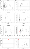 |
Fig. 2 Reduced magnitude of (a) 322966, (b) 323173, (c) 2009 KF37, (d) 275618, (e) 2017 QO33, (f) 54598, (g) 2000 CN152, and (h) 2014 SS303. The vertical line on the left indicates the perihelion distance of the object. In some cases, a vertical line is also plotted to the right, indicating the aphelion distance. The dotted horizontal line shows the MPC catalog absolute magnitude, which it is taken as a reference. The empty symbols correspond to observations made before passing through perihelion (f > 180°), and filled symbols correspond to observations after perihelion passage (f < 180°). The data plotted with triangles correspond to large surveys, black circles correspond to any other MPC data, and red squares show the data obtained in this work. The scales are different for each image because they are adjusted to the data values of each object. |
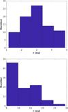 |
Fig. 3 Histogram of the heliocentric distances of the observed ACOs between 0 and 5 au (top) and at more than 5 au (bottom). |
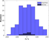 |
Fig. 4 Histogram of the true anomalies of observed ACOs with and without activity. |
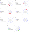 |
Fig. 5 Orbits of (a) 133P, (b) 259P, (c) 311P, (d) 331P, (e) 324P, (f) 354P, and (g) P2015 X6. The black lines represent the orbits of the planets, the blue line shows the orbit of the object, the blue circle shows its perihelion, the red asterisks show the places where activity has been observed, the green asterisks represent the observations made during this work in which activity was confirmed, and the cyan asterisks indicate were no activity was found. The view is from the north ecliptic pole, so that the movement of the objects in their orbits is counterclockwise. |
6 Conclusions and future work
The objective of this work was to monitor the possible activity of ACOs and AAs. We started from a dataset that was analyzed in 2015 and 2016 and extended the list of studied objects to achieve a significant sample. We worked with images obtained from different databases, as well as with new observations made between 2019 and 2021.
We increased the ACO sample of analyzed objects from 7% to 23% compared to the previous work. Our results indicate that a majority fraction within the ACOs-JF population (~400) might be escaped asteroids, with a few cases of dormant comets.
The AA sample was increased to 32% of the known objects. Of the 7 objects we studied, 4 were active in the images. Some objects were active in regions in which activity was observed before, while others were inactive in the same regions or close to them.
Although the sample of objects we studied was considerably extended and allowed us to gain a more complete picture of transitional objects, we understand that there are currently several open questions that could be addressed as future work. For a more conclusive understanding of the nature of ACOs, a comprehensive analysis is imperative. This should encompass an in-depth analysis of the dynamic pathways leading from the main asteroid belt to the chaotic dynamics observed in ACOs. Additionally, a thorough investigation of the relative contributions from different populations and a spectroscopic comparison between ACOs-JF and their source populations are essential components of this analysis.
Furthermore, an exploration of the various mechanisms that cause the activation of asteroids is also necessary. Through such an analysis, we can move closer to a definitive conclusion about the nature of activity in these bodies.
Finally, first results from the recent NASA-DART mission to the Dydimos-Dimorphos binary system show that an artificially activated asteroid was generated (Li et al. 2023), as proposed by Tancredi et al. (2023). The duration of the increase in brightness with respect to the pre-impact magnitude and the evolution of the dust tail helps us better understand the activation process of an asteroid (Li et al. 2023).
Activated asteroid observations.
Acknowledgements
Based on observations collected at the European Southern Observatory under ESO programmes: 60.A-9203(B), 65.S-0184(A), 072.C-0483(B), 079.C-0653(B), 079.C-0670(A), 086.C-0738(A), 095.C-0932(A), 097.C-0912(A), 098.C-0903(B), 099.C-0787(B), 0101.C-0740(A), 167.C-0340(G), 178.C-0036(N), 178.C-0867(G), 178.C-0867(M), 178.C-0867(M), 178.C-0867(T), 278.C-5066(B), 297.C-5060(D), 297.C-5060(E) and 596.C-0822(A). S.M. and G.T. acknowledge financial support from the projects Grupos I+D Ciencias Planetarias C630-348 & C308-347 of the Comisión Sectorial de Investigación Científica (CSIC, Udelar, Uruguay), and the Programa de las Ciencias Básicas (PEDECIBA-MEC, Uruguay). The authors are grateful to the IMPACTON team (T. Rodrigues, R. Souza, A. da Silva, A. Santiago and J. Silva) for the technical support. E.R. would like to thank FAPERJ for its support through a fellowship (E-26/2024.602/2021) and a grant (E-26/201.001/2021). We thank M.E.-S., H.M. and F.W.M. for their observations at OASI in 2019 and 2020. Funding for the DES Projects has been provided by the U.S. Department of Energy, the U.S. National Science Foundation, the Ministry of Science and Education of Spain, the Science and Technology Facilities Council of the United Kingdom, the Higher Education Funding Council for England, the National Center for Supercomputing Applications at the University of Illinois at Urbana-Champaign, the Kavli Institute of Cosmological Physics at the University of Chicago, the Center for Cosmology and Astro-Particle Physics at the Ohio State University, the Mitchell Institute for Fundamental Physics and Astronomy at Texas A&M University, Financiadora de Estudos e Projetos, Fundação Carlos Chagas Filho de Amparo à Pesquisa do Estado do Rio de Janeiro, Conselho Nacional de Desenvolvimento Científico e Tecnológico and the Ministério da Ciência, Tecnologia e Inovação, the Deutsche Forschungsgemeinschaft and the Collaborating Institutions in the Dark Energy Survey. The Collaborating Institutions are Argonne National Laboratory, the University of California at Santa Cruz, the University of Cambridge, Centro de Investigaciones Energéticas, Medioambientales y Tecnológicas-Madrid, the University of Chicago, University College London, the DES-Brazil Consortium, the University of Edinburgh, the Eidgenössische Technische Hochschule (ETH) Zürich, Fermi National Accelerator Laboratory, the University of Illinois at Urbana-Champaign, the Institut de Ciències de l’Espai (IEEC/CSIC), the Institut de Física d’Altes Energies, Lawrence Berkeley National Laboratory, the Ludwig-Maximilians-Universität München and the associated Excellence Cluster Universe, the University of Michigan, NSF’s NOIRLab, the University of Nottingham, The Ohio State University, the University of Pennsylvania, the University of Portsmouth, SLAC National Accelerator Laboratory, Stanford University, the University of Sussex, Texas A&M University, and the OzDES Membership Consortium. Based in part on observations at Cerro Tololo InterAmerican Observatory at NSF’s NOIRLab (NOIRLab Prop. ID 2012B-0001; PI: J. Frieman), which is managed by the Association of Universities for Research in Astronomy (AURA) under a cooperative agreement with the National Science Foundation. The DES data management system is supported by the National Science Foundation under Grant Numbers AST-1138766 and AST-1536171. The DES participants from Spanish institutions are partially supported by MICINN under grants ESP2017-89838, PGC2018-094773, PGC2018-102021, SEV-2016-0588, SEV-2016-0597, and MDM-2015-0509, some of which include ERDF funds from the European Union. IFAE is partially funded by the CERCA program of the Generalitat de Catalunya. Research leading to these results has received funding from the European Research Council under the European Union’s Seventh Framework Program (FP7/2007-2013) including ERC grant agreements 240672, 291329, and 306478. Contribution statements: S.M. is lead author, responsible for the development of code, image analysis, and data processing. G.T. had also contributed to the development of code, writing, and editing of the manuscript. The following authors had provided data from different observatories and archival data: M.B-H. and J.C. from DES, E.R. from OASI, and J.L. from IAC. They reviewed the manuscript, and suggested several improvements.
Appendix A Observational data of studied objects
Observational information regarding ACOs is presented in Table A.1, while that related to AAs can be found in Table A.2. Tables contain date of observation, geocentric distance (Δ), heliocentric distance (r), true anomaly (f), and observatory used.
Observational information for ACOs.
Observational information for AAs.
References
- Alvarez-Candal, A. 2013, A&A, 549, 10 [Google Scholar]
- Alvarez-Candal, A., & Roig, F. 2005, IAU Colloq., 197, 205 [Google Scholar]
- Appenzeller, I., Fricke, K., Fürtig, W., et al. 1998, The Messenger, 94, 1 [NASA ADS] [Google Scholar]
- Belskaya, I. N., Bagnulo, S., Barucci, M. A., et al. 2010, Icarus, 210, 472 [NASA ADS] [CrossRef] [Google Scholar]
- Bolin, B., Denneau, L., Veres, P., et al. 2013, Centr. Bur. Elec. Tel., 3559, 1 [Google Scholar]
- Chandler, C. O., Kueny, J. K., Trujillo, C. A., Trilling, D. E., & Oldroyd, W. J. 2020, ApJ, 892, L38 [Google Scholar]
- Chandler, C. O., Trujillo, C. A., Oldroyd, W. J., et al. 2024, AJ, 167, 156 [Google Scholar]
- DeMeo, F., & Binzel, R. P. 2008, Icarus, 194, 436 [NASA ADS] [CrossRef] [Google Scholar]
- DeMeo, F. E., & Carry, B. 2014, Nature, 505, 629 [NASA ADS] [CrossRef] [Google Scholar]
- DeMeo, Fornasier, S., Barucci, M. A., et al. 2008, AAS/Div. Planet. Sci. Meeting Abs., 40, 47.05 [Google Scholar]
- Díaz, C. G., & Gil-Hutton, R. 2008, A&A, 487, 363 [NASA ADS] [CrossRef] [EDP Sciences] [Google Scholar]
- Di Sisto, R. P., Brunini, A., Dirani, L. D., & Orellana, R. B. 2003, Boletin de la Asociacion Argentina de Astronomia La Plata Argentina, 46, 11 [Google Scholar]
- Di Sisto, R. P., Brunini, A., Dirani, L. D., & Orellana, R. B. 2005, Icarus, 174, 81 [NASA ADS] [CrossRef] [Google Scholar]
- Di Sisto, R. P., Fernández, J. A., & Brunini, A. 2009, Icarus, 203, 140 [Google Scholar]
- Di Sisto, R. P., Ramos, X. S., & Gallardo, T. 2019, Icarus, 319, 828 [NASA ADS] [CrossRef] [Google Scholar]
- Doressoundiram, A., Barucci, M. A., Tozzi, G. P., et al. 2005, Planet. Space Sci., 53, 1501 [Google Scholar]
- Elst, E. W., Pizarro, O., Pollas, C., et al. 1996, IAU Circ., 6456, 1 [NASA ADS] [Google Scholar]
- Everhart, E. 1985, Astrophys. Space Sci. Lib., 115, 185 [NASA ADS] [CrossRef] [Google Scholar]
- Fernández, Y. R., Jewitt, D. C., & Sheppard, S. S. 2005, AJ, 130, 308 [Google Scholar]
- Fernández, J. A., Sosa, A., Gallardo, T., & Gutiérrez, J. N. 2014, Icarus, 238, 1 [CrossRef] [Google Scholar]
- Flaugher, B., Diehl, H. T., Honscheid, K., et al. 2015, AJ, 150, 150 [Google Scholar]
- Geem, J., Ishiguro, M., Bach, Y. P., et al. 2022, A&A, 658, A158 [NASA ADS] [CrossRef] [EDP Sciences] [Google Scholar]
- Gwyn, S. D. J., Hill, N., & Kavelaars, J. J. 2012, PASP, 124, 579 [NASA ADS] [CrossRef] [Google Scholar]
- Hsieh, H. H. 2017, Phil. Trans. R. Soc. London Ser. A, 375, 2097 [Google Scholar]
- Hsieh, H. H., & Haghighipour, N. 2016, Icarus, 277, 19 [NASA ADS] [CrossRef] [Google Scholar]
- Hsieh, H. H., & Jewitt, D. 2006, Science, 312, 561 [NASA ADS] [CrossRef] [Google Scholar]
- Hsieh, H. H., Jewitt, D. C., & Fernández, Y. R. 2004, AJ, 127, 2997 [NASA ADS] [CrossRef] [Google Scholar]
- Hsieh, H. H., Jewitt, D., Lacerda, P., Lowry, S. C., & Snodgrass, C. 2010, MNRAS, 403, 363 [NASA ADS] [CrossRef] [Google Scholar]
- Hsieh, H. H., Ishiguro, M., Kim, Y., et al. 2017, AAS/Div. Planet. Sci. Meeting Abs., 49, 305.10 [Google Scholar]
- Jewitt, D., & Hsieh, H. H. 2024, in Comets III, eds. K. J. Meech, M. R. Combi, D. Bockelée-Morvan, S. N. Raymodn, & M. E. Zolensky (Tucson: University of Arizona Press), 767 [Google Scholar]
- Jewitt, D., & Luu, J. 1989, AJ, 97, 1766 [Google Scholar]
- Kim, Y., Ishiguro, M., & Usui, F. 2014, ApJ, 789, 151 [NASA ADS] [CrossRef] [Google Scholar]
- Kresak, L. 1979, Dynamical Interrelations Among Comets and Asteroids., eds. T. Gehrels, & M. S. Matthews (Tucson:, University of Arizona Press), 289 [Google Scholar]
- Li, J., Hirabayashi, M., Farnham, T., et al. 2023, Nature, 616, 452 [NASA ADS] [CrossRef] [Google Scholar]
- Licandro, J., Alvarez-Candal, A., de León, J., et al. 2008, A&A, 481, 861 [NASA ADS] [CrossRef] [EDP Sciences] [Google Scholar]
- Licandro, J., Alí-Lagoa, V., Tancredi, G., & Fernández, Y. 2016, A&A, 585, A9 [NASA ADS] [CrossRef] [EDP Sciences] [Google Scholar]
- Licandro, J., Popescu, M., de León, J., et al. 2018, A&A, 618, A170 [NASA ADS] [CrossRef] [EDP Sciences] [Google Scholar]
- Lorin, O., & Rousselot, P. 2007, MNRAS, 376, 881 [Google Scholar]
- Luu, J. X. 1992, Icarus, 97, 276 [NASA ADS] [CrossRef] [Google Scholar]
- Martino, S., Tancredi, G., Monteiro, F., Lazzaro, D., & Rodrigues, T. 2019, Planet. Space Sci., 166, 135 [NASA ADS] [CrossRef] [Google Scholar]
- Rickman, H., Fernández, J. A., & Gustafson, B. A. S. 1990, A&A, 237, 524 [Google Scholar]
- Romon-Martin, J., Barucci, M. A., de Bergh, C., et al. 2002, Icarus, 160, 59 [Google Scholar]
- Rondón, E., Lazzaro, D., Rodrigues, T., et al. 2020, PASP, 132, 065001 [CrossRef] [Google Scholar]
- Seligman, D. Z., Farnocchia, D., Micheli, M., et al. 2023, PSJ, 4, 35 [NASA ADS] [Google Scholar]
- Simion, G., Popescu, M., Licandro, J., Vaduvescu, O., & de León, J. 2020, European Planetary Science Congress, 351 [Google Scholar]
- Tancredi, G. 2014, Icarus, 234, 66 [NASA ADS] [CrossRef] [Google Scholar]
- Tancredi, G., Lindgren, M., & Rickman, H. 1990, A&A, 239, 375 [NASA ADS] [Google Scholar]
- Tancredi, G., Liu, P.-Y., Campo-Bagatin, A., Moreno, F., & Domínguez, B. 2023, MNRAS, 522, 2403 [Google Scholar]
- Tozzi, G.-P., Bagnulo, S., Barucci, M. A., et al. 2012, AAS/Div. Planet. Sci. Meeting Abstracts, 44, 310.15 [Google Scholar]
- Tubbiolo, A. F., Bressi, T. H., Wainscoat, R. J., et al. 2015, Minor Planet Electronic Circulars, 2015-X180 [Google Scholar]
- Vaduvescu, O., Popescu, M., Comsa, I., et al. 2013, Astron. Nachr., 334, 718 [NASA ADS] [CrossRef] [Google Scholar]
- Ye, Q.-Z., Brown, P. G., & Pokorný, P. 2016, MNRAS, 462, 3511 [NASA ADS] [CrossRef] [Google Scholar]
All Tables
All Figures
|
Fig. 1 Surface brightness profiles of (a) 29981 (VLT), (b) 54598 (IMPACTON), (c) 90572 (IMPACTON), (d) 515718 (DES), (e) 2015 BK22 (IMPACTON), (f) 2014 OG392 (DES), (g) 2016 YB13 (DES), (h) 259 P (DES), (i) 311 P (DES), and (j) P/2015 X6 (DES). The plots show the normalized intensity values of each pixel from the centroid for one or more stars (blue dots), the Moffat fit of the stars (red line), the normalized intensity values of the object (green dots), and the Moffat fit of the object (black line). The red error bars correspond to the stars and the black error bars to the object. The errors were calculated from the dispersion of the flux values with respect to the fit. A small artificial horizontal offset has been introduced in the position of the bars to avoid overlap. In the image header we list the object name, date, image range (when a set of images was coadded), image number or time, and the calculated magnitude. When the object appeared as a trail (2016 YB13), the intensity values of the trail are plotted superimposed with the profile of the stars (with their Moffat fit). |
| In the text | |
|
Fig. 2 Reduced magnitude of (a) 322966, (b) 323173, (c) 2009 KF37, (d) 275618, (e) 2017 QO33, (f) 54598, (g) 2000 CN152, and (h) 2014 SS303. The vertical line on the left indicates the perihelion distance of the object. In some cases, a vertical line is also plotted to the right, indicating the aphelion distance. The dotted horizontal line shows the MPC catalog absolute magnitude, which it is taken as a reference. The empty symbols correspond to observations made before passing through perihelion (f > 180°), and filled symbols correspond to observations after perihelion passage (f < 180°). The data plotted with triangles correspond to large surveys, black circles correspond to any other MPC data, and red squares show the data obtained in this work. The scales are different for each image because they are adjusted to the data values of each object. |
| In the text | |
|
Fig. 3 Histogram of the heliocentric distances of the observed ACOs between 0 and 5 au (top) and at more than 5 au (bottom). |
| In the text | |
|
Fig. 4 Histogram of the true anomalies of observed ACOs with and without activity. |
| In the text | |
|
Fig. 5 Orbits of (a) 133P, (b) 259P, (c) 311P, (d) 331P, (e) 324P, (f) 354P, and (g) P2015 X6. The black lines represent the orbits of the planets, the blue line shows the orbit of the object, the blue circle shows its perihelion, the red asterisks show the places where activity has been observed, the green asterisks represent the observations made during this work in which activity was confirmed, and the cyan asterisks indicate were no activity was found. The view is from the north ecliptic pole, so that the movement of the objects in their orbits is counterclockwise. |
| In the text | |
Current usage metrics show cumulative count of Article Views (full-text article views including HTML views, PDF and ePub downloads, according to the available data) and Abstracts Views on Vision4Press platform.
Data correspond to usage on the plateform after 2015. The current usage metrics is available 48-96 hours after online publication and is updated daily on week days.
Initial download of the metrics may take a while.