| Issue |
A&A
Volume 698, June 2025
|
|
|---|---|---|
| Article Number | A176 | |
| Number of page(s) | 18 | |
| Section | Numerical methods and codes | |
| DOI | https://doi.org/10.1051/0004-6361/202553990 | |
| Published online | 17 June 2025 | |
How to make CLEAN variants faster using clustered components informed by the autocorrelation function
1
Max-Planck-Institut für Radioastronomie,
Auf dem Hügel 69,
53121
Bonn,
Germany
2
National Radio Astronomy Observatory,
PO Box O,
Socorro,
NM
87801,
USA
★ Corresponding author: This email address is being protected from spambots. You need JavaScript enabled to view it.
Received:
31
January
2025
Accepted:
22
April
2025
Abstract
Context. The deconvolution, imaging, and calibration of data from radio interferometers is a challenging computational (inverse) problem. The upcoming generation of radio telescopes poses significant challenges to existing and well-proven data reduction pipelines, due to the large data sizes expected from these experiments and the high resolution and dynamic range.
Aims. In this manuscript, we deal with the deconvolution problem. A variety of multiscalar variants to the classical CLEAN algorithm (the de facto standard) have been proposed in the past, often outperforming CLEAN at the cost of significantly increasing numerical resources. For this work our aim was to combine some of these ideas for a new algorithm, Autocorr-CLEAN, to accelerate the decon-volution, and to prepare the data reduction pipelines for the data sizes expected from the upcoming generation of instruments.
Methods. To this end, we propose using a cluster of CLEAN components fitted to the autocorrelation function of the residual in a subminor loop, to derive continuously changing and potentially nonradially symmetric basis functions for CLEANing the residual.
Results. Autocorr-CLEAN allows the superior reconstruction fidelity achieved by modern multiscalar approaches, and their superior convergence speed. It achieves this without utilizing any substeps of super-linear complexity in the minor loops, keeping the single minor loop and subminor loop iterations at an execution time comparable to that of CLEAN. Combining these advantages, Autocorr-CLEAN is found to be up to a magnitude faster than the classical CLEAN procedure.
Conclusions. Autocorr-CLEAN fits well in the algorithmic framework common for radio interferometry, making it relatively straightforward to include in future data reduction pipelines. With its accelerated convergence speed, and smaller residual, Autocorr-CLEAN may be an important asset for data analysis in the future.
Key words: methods: numerical / techniques: high angular resolution / techniques: image processing / techniques: interferometric / galaxies: jets / galaxies: nuclei
© The Authors 2025
 Open Access article, published by EDP Sciences, under the terms of the Creative Commons Attribution License (https://creativecommons.org/licenses/by/4.0), which permits unrestricted use, distribution, and reproduction in any medium, provided the original work is properly cited.
This article is published in open access under the Subscribe to Open model.
Open Access funding provided by Max Planck Society.
1 Introduction
In radio interferometry, the signal recorded by an antenna pair observing the same source simultaneously is correlated. This correlation product (referred to as visibility) is approximated by the Fourier transform of the true sky brightness distribution with a spatial frequency determined by the baseline projected to the sky plane. Because the Earth is rotating, the relative position of the antennas to the sky plane is changing, and the Fourier domain (also called the uv-domain) gets filled swiftly, a procedure usually referred to as aperture synthesis (Thompson et al. 2017).
The imaging problem (i.e., deriving an image from the observed visibilities) is a challenging ill-posed inverse problem. The challenges arise from the fact that only a subset of all possible Fourier coefficients is measured on a non-Euclidean grid, the observations are disturbed by instrumental noise, and a variety of calibration effects need to be corrected, including atmospheric delays described by station-based gains, radio frequency interference (RFI), or wide-field and wide-band effects. In the usual algorithm architecture that is adopted by almost all major radio interferometers in the world, this problem is solved by a sequential application of loops and projections that are nested around each other. For instance, the problem of recovering a model from sparse measurements of the visibilities is typically reformulated as a deconvolution algorithm (i.e., the minor loop) solved by an iterative matching pursuit known as CLEAN deconvolution (Högbom 1974). The gridding-degridding step (i.e., gridding visibilities on a regular grid and applying the inverse fast Fourier transform) is usually called the major loop. The overall procedure calls the major loop multiple times, and internally the minor loop, as first proposed by Schwab (1984). The minor-major loop cycle is itself looped in outer self-calibration loops (solving for gains), wide-field and wide-band projections, and RFI mitigation procedures.
Currently, for most experiments gridding is the biggest bottleneck in the data analysis, especially for the data sizes that may be expected from the next generation of radio interferometers such as the ngVLA (Bhatnagar et al. 2021). The ngVLA is a project proposed to replace the VLA, and will combine (following its current plans) a dense core of stations, providing a wide field of view, with intermediate baselines and continental baselines as currently only available with very long baseline interferometry (VLBI) experiments. Significant progress has been made in scaling the major loops up to the performance needed for future arrays by the efficient parallelization of this step on GPUs on major computing facilities (Bhatnagar et al. 2022; Kashani et al. 2023). Since the numerical cost for the deconvolution scales with the number of pixels (and the number of pixels with relevant intensity information is expected to be large for the upcoming generation of radio telescopes, due to the combination of short and long baselines and an increased sensitivity), the time performance of the deconvolution step becomes a secondary focus area of pipeline acceleration again. As outlined above, the actual deconvolution is the innermost loop, and is thus an operation that is called multiple times throughout the data analysis pipeline. Any solution that allows cleaning deeper at every minor cycle at the cost of an acceptable time increase will be of great importance to reduce overall computational time, at least by reducing the number of major loops. Moreover, it has been noted that the minor loop may dominate the major loop for some experiments that deal with exceptionally large image cubes, for example for spectral reductions in ALMA data (see, e.g., for the latest run-time performance benchmarks Kepley et al. 2023). This situation may get worse when the size of data cubes increases with the wide-band sensitivity upgrade.
The de facto standard used to solve the deconvolution problem is CLEAN (Högbom 1974; Clark 1980; Schwab 1984). CLEAN is a matching pursuit approach that iteratively searches for the peak in the current residual, and substitutes a shifted and rescaled version of the point spread function from the residual. CLEAN remains the fastest imaging algorithms, and one of the most robust. This is mainly caused by the fact that in a single CLEAN iteration no convolution operation needs to be performed, but rather simple substitution steps only. Moreover, CLEAN fits well in the proven current data processing pipelines, while most novel approaches still need to demonstrate that they can handle all the necessary calibration steps and imaging modes in their respective paradigms. In this manuscript we focus on the numerical performance of the minor loop. We developed a version of the CLEAN algorithm that fits well in current data processing pipelines, and primarily exceeds classical CLEAN approaches in terms of convergence speed and depth of the CLEANing.
CLEAN has been adapted over the years to a variety of settings, most remarkably to multiscale versions (Bhatnagar & Cornwell 2004; Cornwell 2008; Rau & Cornwell 2011; Offringa et al. 2014; Offringa & Smirnov 2017; Müller & Lobanov 2023b) in which extended multiscalar functions are fitted to the data rather than point sources being fitted to the data. Multiscalar versions of CLEAN correct successfully for the biggest limitation of the CLEAN algorithm, namely that the spatial correlation between pixels is not taken into account. MS-CLEAN versions usually perform better than standard CLEAN, particularly when extended diffuse emission is present in the data. Moreover, while a single minor loop iteration may take more time for MS-CLEAN since it needs to survey through multiple scalarized image channels, the overall number of iterations, and the number of major loops is typically smaller.
One of the prevailing open questions for MS-CLEAN alternatives to CLEAN is how to choose the basis functions that are used to represent the image. This is also the area of algorithmic developments that may allow the biggest improvements. A number of approaches have been proposed, ranging from predefined sets of tapered truncated parabola (Cornwell 2008) or Gaussian basis functions as implemented in CASA (CASA Team 2022); multiresolution CLEAN with hierarchically decreasing tapers (Wakker & Schwarz 1988) over specially designed wavelets (Starck et al. 1994; Müller & Lobanov 2022, 2023b), following the ideas pioneered by compressive sensing for radio interferometry (Starck et al. 2002, 2005; Wiaux et al. 2009); and ideas revolving around multiresolution support (Offringa & Smirnov 2017; Müller & Lobanov 2023a) and components model-fitted to the residual (Bhatnagar & Cornwell 2004; Zhang et al. 2016; Hsieh & Bhatnagar 2021). While nonradially symmetric basis functions are used routinely for compressive sensing approaches (see, e.g., the reviews in Starck & Murtagh 2006; Starck et al. 2015), out of the aforementioned options for CLEAN methods only DoB-CLEAN (Müller & Lobanov 2023b) includes elliptical basis functions that break the radial symmetry. This option may improve the image compression, particularly when the source structure is nonradially symmetric, as is common for resolved sources. Moreover, elliptical basis functions are shown to be useful in more exotic configurations with large gaps (as usual for VLBI) and highly elliptical point spread functions (Müller & Lobanov 2023b). Moreover, only Asp-CLEAN (Bhatnagar & Cornwell 2004) adapts the scales continuously, while almost all other approaches rely on a fixed discretized set of functions. As a drawback, the continuous adaptation step within Asp-CLEAN takes a considerable amount of time since a nonlinear optimization problem needs to be solved by explicit gradient-based minimization algorithms, an issue that was addressed in recent implementations of the scheme (Zhang et al. 2016; Hsieh & Bhatnagar 2021) by an approximate version of the convolution point spread function.
In this manuscript, describe how we combined several of these advantages. We constructed a novel MS-CLEAN algorithm that allows for the fitting of nonradial basis functions, adapts the form of the model components continuously, and retains the speed achieved by limiting the algorithm to substitution and shifting operations only. To this end, we propose using the autocorrelation function of the residual (i.e., in image space the mirrored convolution of the residual with itself) as a selection criterion for the model components. We used a model component whose autocorrelation function approximates the autocorrelation function of the true sky brightness distribution (which is not limited to radially symmetric configurations). We chose the autocorrelation function here as a criterion inspired by Bayesian arguments; in other words, we wanted to fit the residual with a Gaussian field with a covariance matrix matching the covariance of true on-sky emission. Additionally, the autocorrelation function has some practical advantages over adapting the model components directly to the residual (e.g., as done for Asp-CLEAN). It encodes global information about the shape of emission structures that can be shared between multiple features in the image, is peaked by definition at the central pixel, and is point-symmetric.
Since the autocorrelation function of the residual contains artifacts of the point spread function also present in the residual itself, a simultaneous CLEANing of the autocorrelation function, and the actual image is needed in an alternating fashion. First, we approximate the autocorrelation of the true sky brightness distribution, use this approximation to perform a MS-CLEAN minor loop iteration, update the residual and the autocorrelation function, and proceed with the first step. Since the autocorrelation function will be approximated by CLEAN components, the MS-CLEAN step will fit clusters and/or clouds of CLEAN components rather than individual CLEAN components, which contributes to a significant acceleration of the minor cycle.
The new algorithm, called Autocorr-CLEAN, fits the multiple CLEAN components at every iteration simultaneously, informed by the autocorrelation of the residual, while avoiding any explicit computation of the convolution. In total, every single minor loop iteration is as fast as for standard CLEAN, while the number of iterations needed drops significantly. Moreover, the algorithm fits naturally in the framework of major loops and calibration routines developed and routinely applied for the data analysis in radio interferometry. However, we note that the scope of this work is limited to a proof of concept of the idea. We only studied the minor loop, as isolated from the full pipeline as possible. We do not address the application of Autocorr-CLEAN in real scenarios here, which means that we do not discuss the interaction of the deconvolution with grid-ding, calibration, or flagging, and leave these considerations to a future work, and ultimately to gathering experience in practice.
2 Theory
2.1 Radio interferometry
The correlated signal of an antenna pair is approximated by the Fourier transform of the true sky brightness distribution, a relation commonly known as the van-Cittert-Zernike theorem. This relation is only an approximation that neglects the projection ofa wide field of view on a plane (commonly expressed by w-terms). The gridding step translates the problem of recovering an image from sparsely represented Fourier data into a deconvolution problem with an effective point spread function BD:
 (1)
(1)
We refer to the point spread function as the dirty beam, and to the map produced from the gridded visibilities as the dirty map. The goal of the deconvolution operation (also known as the minor loop) is to retrieve the image I that describes the data, which is the setting that we work in for the remainder of this manuscript.
A variety of instrumental and astrophysical corruptions affect the observed data, for example thermal noise, station-based gains describing atmospheric limitations, and the more challenging direction-dependent or baseline-dependent effects. The latter are typically taken into account during the gridding operation by projection algorithms (e.g., Bhatnagar et al. 2008, 2013; Bhatnagar & Cornwell 2017; Tasse et al. 2013; Offringa et al. 2014). Moreover, self-calibration needs to be performed alternating with the minor loop operations as well, and directly affects the observed visibilities, and in turn the gridded visibilities. Hence, these corruption effects are taken into account outside of the minor loop operation, leaving deconvolution as a pristine problem that can be studied individually. This modularized strategy has proven crucial in order to adapt the technique of aperture synthesis over the decades for a variety of instruments.
As outlined in Sect. 1, the minor loop may become a performance bottleneck again in future data analysis pipelines because it is the innermost loop in a nested system of loops, and needs to be called multiple times (although it is believed that in many cases the gridding cost exceeds the deconvolution cost). This may be true especially for arrays that process big image cubes. In this manuscript we discuss the deconvolution problem on its own detached from the larger picture of the data analysis.
2.2 CLEAN and MS-CLEAN
CLEAN (Högbom 1974) is the standard deconvolution algorithm that was used in the past. It has seen various versions and adaptations (Clark 1980; Schwab 1984; Bhatnagar & Cornwell 2004; Cornwell 2008; Rau & Cornwell 2011; Offringa et al. 2014; Offringa & Smirnov 2017; Müller & Lobanov 2023b), but the basic outline remains mostly the same. In an iterative fashion, we search for the maximum peak in the current residual, shift the point spread function to that position, scale the point spread function, and subtract the point spread function from the residual. The output of the CLEAN algorithm is a list of the CLEAN components (point sources) and the final residual, which are combined by convolving the list of CLEAN components with the clean beam (a Gaussian approximation to the main lobe of the point spread function) into a final image. CLEAN remains the fastest deconvolution algorithm, specifically since during the minor loop iterations only relatively inexpensive numerical operations need to be performed, in contrast to most forward-modeling techniques.
Multiscale versions of CLEAN (MS-CLEAN) basically replace the CLEAN components by multiscalar components and search the residual not only along the pixels in the residual, but also across multiple spatial channels (the residual convolved with a specific spatial scale). In its basic outline, and especially when working on a predefined set of scales, the search products and the cross-correlations between multiple scales can be pre-computed during the initialization of the calculation and the CLEANing is done in channels without explicit convolutions during the minor cycles (see, e.g., the discussion in Cornwell 2008).
In many situations, MS-CLEAN approaches outperform CLEAN, especially for the representation of extended emission. This superior performance is achieved since the MS-CLEAN components process spatial correlations between pixels missing from the standard CLEAN interpretations. Classical MS-CLEAN (Cornwell 2008) iterations remain at an acceptable speed compared to regular CLEAN. This is particularly achieved since the subtraction step within the different scalarized channels can be computed in parallel. Since a single MS-CLEAN component essentially replaces the need for dozens or hundreds of regular CLEAN components (depending on the spatial scale that is processed), MS-CLEAN algorithms typically need a smaller number of iterations to converge. This property (an increased speed of convergence in terms of the number of iterations) is the main benefit that we are interested in throughout this manuscript.
It has been demonstrated that (MS-)CLEAN, while being a matching pursuit approach, can be understood essentially as a compressive sensing algorithm (Lannes et al. 1997; Starck et al. 2002) in the sense that the algorithm tries to find a representation of the data with as few model components as possible (i.e., essentially a sparse representation). Hence, the performance of MS-CLEAN approaches is linked to the sparsifying properties of the basis in use. This is particularly true for the number of generations needed to achieve convergence, and thus the runtime of the algorithm. When we model the image by a dictionary of basis functions that allow a sparser representation, we ultimately need fewer model components to represent the image, and hence fewer minor loop iterations.
Two MS-CLEAN variants stand out as particular useful developments in this direction. First, DoB-CLEAN was proposed by Müller & Lobanov (2023b) on the basis of the DoG-HiT algorithm (Müller & Lobanov 2022) that found successful application in a variety of VLBI experiments (e.g., Müller & Lobanov 2023a; Kramer et al. 2025; Roelofs et al. 2023; Event Horizon Telescope Collaboration 2024; Paraschos et al. 2024; Kim et al. 2025; Müller 2024) and related fields (Müller et al. 2024). The approach is the first MS-CLEAN algorithm that develops basis functions that are not necessarily radially symmetric, as may be crucial in the presence of resolved nonradially symmetric source structures. This has been achieved by the use of direction-dependent wavelets modeled by the difference of elliptical Gaussians. Second, Asp-CLEAN, originally proposed by Bhatnagar & Cornwell (2004) and subsequentially efficiently implemented and improved by Zhang et al. (2016); Hsieh & Bhatnagar (2021), is the first MS-CLEAN variant that models the emission via a continuous set of basis functions. This is achieved by substep fitting the scalarized basis functions continuously to minimize the residual. This additional flexibility holds significant compressing properties and is the reason for the high accuracy of the algorithm. As a drawback, the increase in numerical cost stemming from the continuous adaptation of the basis function is significant.
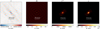 |
Fig. 1 Autocorrelation of the initial residual ( |


3 Autocorr-CLEAN
3.1 Overview and idea
In this manuscript we discuss the design of a novel MS-CLEAN variant, Autocorr-CLEAN, which draws a superior performance from the use of basis functions that are continuously adapted to the current residual, and potentially elliptical in the spirit of compressive sensing. Moreover, it should remain competitive in terms of running time compared to standard CLEAN and MS-CLEAN by avoiding any optimization step that includes the evaluation of the Fourier transform, gridding-degridding, or a convolution operation in its interior iterations.
To this end, we derived an ad hoc approximation to the ideal basis function to model the current residual (ideal in the sense that it models the final image with the smallest number of components). This question is closely related to the autocorrelation function of the residual. If the residual is dominated by diffuse emission, the autocorrelation function is expected to be wide. If vice versa the residual is dominated by point sources, the main lobe of the autocorrelation function would be point-like as well. If we know the auto-correlation function of the true sky brightness distribution, this will provide a powerful heuristics to select a basis function during the minor loop. The most natural choice would be to use Gaussians with exactly this covariance matrix. This is the idea that we are following in this manuscript. The autocorrelation of the residual ID is given by
 (2)
(2)
where we used the notation  , and ⋆ is the convolution.
Similar ideas are explored by Bayesian algorithms when the prior distribution is fixed or by the most straightforward neural network approaches in which the autocorrelation of the image structures is learned through some training data (e.g., Schmidt et al. 2022). However, the challenge with such direct applications arises from the fact that the exact correlation structure is typically not known a priori. That led recently to the development of Bayesian algorithms that infer the correlation structure together with the image (e.g., Junklewitz et al. 2016; Arras et al. 2021) and to neural network approaches that utilize generative models to construct the prior during the imaging (e.g., Gao et al. 2023) or enhance the network on the current residual in a network series (Aghabiglou et al. 2024).
Translated into the language of the MS-CLEAN framework, we did not know the autocorrelation function of the true sky-brightness distribution a priori, but we wanted to model it simultaneously with the CLEANing of the actual image structure. Then we used the current autocorrelation model to design a MS-CLEAN component used during the CLEANing of the residual. The autocorrelation function of the residual poses a deconvolution problem that is fairly similar to the actual imaging problem by combining Eqs. (1) and (2):
 (3)
(3)
Hence, we can get an approximation to the current autocorrelation function of the residual (or at least its main lobe) by solving the deconvolution problem in Eq. (3) with standard CLEAN iterations. This leads to the description of the autocorrelation II by a list of delta components. In the next step, we used this cloud of components as a MS-CLEAN component to clean the residual.
The overall algorithmic framework consists of the following steps:
Solving a problem (3) approximately via CLEAN, yielding a list of CLEAN components
 approximating II.
Performing a MS-CLEAN step on the current residual ID with the basis function
 , which means searching for the maximum peak in
  , shift and rescaling the point spread function to this position and substituting
  from the residual.
Updating the autocorrelation function of the updated residual and proceeding with the first step until convergence is achieved.
As an illustrative example, we show the first autocorrelation of the residual (II), the beam (BB), and the point source model  in Fig. 1. These quantities are approximately related to each other by the convolution
  . As outlined below, we use γ = 2 in this example. The first MS-CLEAN model component is shown in the rightmost panel:
  . The example is derived for Cygnus A. We provide more details on the synthetic data set and reconstruction in Sect. 4.
The basis functions о determined in this way change continuously during the imaging procedure, and break potentially radial symmetry (but are necessarily point-symmetric since the autocorrelation function is point-symmetric by definition). In contrast to MS-CLEAN (Cornwell 2008; Rau & Cornwell 2011), Asp-CLEAN (Bhatnagar & Cornwell 2004), or DoB-CLEAN (Müller & Lobanov 2023b), the basis functions are not extended diffuse model components, but clouds of point-like CLEAN components instead. This has the serious drawback that the extended diffuse emission is still represented by pointy model components, which is the issue MS-CLEAN was originally proposed to solve. However, since о still encodes the spatial correlation structure of the current residual, we typically get better performance than the standard CLEAN, as we show below. This is caused by the superior information on the positioning of the single components and their strengths compared to CLEAN achieved by fitting a spatially correlated model о to the residual.
The main benefit that we are aiming for here is the increased numerical speed in comparison to CLEAN, MS-CLEAN, and Asp-CLEAN. This is essentially motivated by the modeling of hundreds of components at once in the update step of the residual. This theoretically gives several orders of magnitude of speedup over CLEAN, under the limiting assumption that the autocorrelation deconvolution is cheap, and no residual errors accumulate over time. We would like to point out a second major difference to the aforementioned multiscale algorithms. Asp-CLEAN derives the shape of the model function locally on the residual (i.e., it fits a Gaussian that reduces the residual ideally at the position of the maximum peak). Autocorr-CLEAN derives the shapes from some global statistics that take into account all the structures in the residual. The first strategy can be expected to subtract a larger fraction of the residual with every iteration. Nevertheless, compared to MS-CLEAN variants we claim a speedup for Autocorr-CLEAN stemming from the consideration that the autocorrelation only changes smoothly as a function of minor loop iterations, allowing a quick update of the autocorrelation model with just a few new model components. This assumption however may also be violated when the dynamic range between large scales and small scales is low.
3.2 Efficient implementation
CLEAN and its multiscalar variants are so fast because they only include operations with linear complexity in their minor loop iterations (i.e., only shifting, rescaling, and substitution). Any evaluation of the Fourier transform or convolution is of superlinear complexity, and takes considerably longer. To maintain the speed of the minor loop iterations as much as possible, we show in this subsection that there is no need to calculate convolutions during the Autocorr-CLEAN minor loop iterations.
It was originally proposed by Cornwell (2008) that all quantities that are necessary for MS-CLEAN could be pre-computed during the initialization. This means that all the convolutions of the point spread function BD with the scales ω0, ω1, ..., and the covariance between the scales  . Every minor loop iteration just needs to reshift, rescale, and substitute the respective covariance product from the channels
  , an operation that could be easily parallelized.
Here, we follow the same strategy; for example, we pre-compute  B for the update step of the residual and iteratively update this property whenever the model о changes. There is one important difference though. Since the autocorrelation function is a second-order function of the residual, its update (when the residual gets updated) is also of second order. For example, if the MS-CLEAN step on the residual computed by the parameter assignment is
 (4)
(4)
then we have to update the autocorrelation function II to second order by
 (5)
(5)
which in itself makes the pre-computation of properties such as  necessary, and so on. Following this strategy, one can derive a full set of pre-computable quantities that avoid the computations of convolution or correlation operations during the minor loop iterations.
We present the pseudocode of the Autocorr-CLEAN algorithm in Algorithm 1. To provide a better overview, we highlight the different logical blocks in Algorithm 1 with different sections. First, we initialize the autocorrelation products by computing an explicit convolution (block 2). We note that this needs to be done only once during the initialization, and could in principle be computed efficiently during the gridding step. Next, we approximate the autocorrelation function by an initial model of CLEAN components (block 3) and initialize all helper products that are needed during the latter iterations (block 4). We note that, while stated differently in Algorithm 1, an explicit convolution does not need to be computed. Since the model ω0 is composed of δ-components, we can add up the shifted rescaled point spread functions instead. This step is in principle not different to block 3 describing the interior loop, but we simplified its writing in Algorithm 1 to maintain a clear overview. The actual CLEANing is done with two nested loops. The exterior loop resembles the classical MS-CLEAN minor loop, except that we restrict ourselves to the basis function co;. After the update step of the residual, we need to update all autocorrelation products that depend directly on the current residual (block5). As outlined above, this is done in an analytic way without the explicit recalculation of a convolution. Among others, the autocorrelation function H was updated. Consequently, we refined the approximation of the autocorrelation in an interior loop (block 6), which we refer to as the subminor loop and updated all the correlation helper functions iteratively. The final list of δi * ωi is an approximation to the true sky brightness distribution. Conveniently, this list could be convolved with the clean beam, as is standard for aperture synthesis.
While the procedure described for Autocorr-CLEAN in this manuscript is the first one that effectively uses the autocorrelation function to find model components, the idea of a subminor loop to cluster components is not new. A similar approach is described in Offringa & Smirnov (2017), and Jarret et al. (2025) recently described a framework in which a subminor loop informs a LASSO problem.
The algorithm has been implemented in the software package LibRA1. LibRA is a project that exposes algorithms used in radio astronomy directly from CASA (McMullin et al. 2007). It is thus well suited for algorithmic development. Vice versa, Autocorr-CLEAN has been implemented in a CASA-friendly environment, which may make the transfer simple.
3.3 Control parameters
Listed in Algorithm 1 are three specific control parameters that we would like to mention: the exterior and interior stopping rules, and the power factor y. In additional, typical CLEAN control parameters such as the gain or the windows need to be taken into account. We note that almost all of these parameters can be interpreted as regularization parameters, and a characterization of their impact on the image structure has been recently analytically described by the Pareto front, as well as several ad hoc selection criteria for navigating this front (Müller et al. 2023; Mus et al. 2024b,a). However, these schemes are computationally very demanding, and thus defy the goal of this work. We instead focus on the discussion of natural strategies on how to choose these control parameters. It should be noted however that the choice of control parameters for CLEAN cannot be studied separated from each other since multiple parameters affect each other. For example, the chosen weighting affects the achievable dynamic range, and hence the heuristics when to stop the minor loop. Moreover, we only study the minor loop in this manuscript and leave the interaction with the major loop for a consecutive work.
Block 1: load the input
Require: Dirty image: 
Require: Psf: BD
Require: Clean beam: C
Require: gain: gain
Require: stopping rules for CLEAN iterations
Require: power parameter: γ
Block 2: initialization of autocorrelation products
▷ Autocorrelation:  (notation:
  )
)
▷ Psf: BB = BD * BD
▷ BI0 = BD * 
Block 3: approximate autocorrelation function by a model
▷ Clean H0 with psf BB
▷ List of components:  approximates
▷ Store model of CLEAN components as 
Block 4: initialize all correlation helper products
▷ 
▷ 
▷ 
▷ 
▷ 
▷ 
▷ 
Loop 1: external MS-CLEAN minor loop on the residual
while  until stopping rule 1 do
▷ Perform MS-CLEAN step with ωi as basis function, searching in MI: 
Block 5: now update all autocorrelation products with the new residual
▷ 
▷ 
▷ 
▷ 
Loop 2: internal Loop to fit updated autocorrelation
▷ 
while  until stopping rule 2 do
▷ perform CLEAN step on updated autocorrelation  with psf BB:
Block 6: update all correlation helper functions
▷ 
▷ 
▷ 
▷ 
▷ 
▷ 
▷ 
end while
▷ 
end while
Ensure: List of CLEAN components convolved with basis functions  is approximating the image
The exterior stopping rule (stopping rule 1) is not particularly different from the stopping rules applied in standard (MS-)CLEAN applications. We stop the cleaning of the residual once we start overfitting. This has been traditionally identified by the recurrent modeling of negative components, the histogram distribution of the residual (i.e., the residual is noise-like), or as recently proposed by the residual entropy (Homan et al. 2024). In principle, these rules also apply to Autocorr-CLEAN.
The application of MS-CLEAN variants to synthetic and real data typically leads to a specific observation. In some cases the large scales are removed first, gradually moving to smaller scales. This is caused by the fact that in most radio arrays the short baselines dominate over the long baselines since the baseline dependent signal-to-noise ratio is higher and there are more short baselines. However, the exact behavior (i.e., which scale is chosen at which points) could differ for every experiment, and is determined by the sensitivity of short baselines compared to long baselines, the amount of small-scale and large-scale structure in the image, the weighting, and the tapering. Furthermore, a manual scale-bias is typically introduced, with the default values favoring small scales over large scales (Cornwell 2008; Offringa & Smirnov 2017). The opposite behavior has been observed for VLBI arrays, which often lack the coverage of short baselines (Müller & Lobanov 2023b). For the dense, connected element interferometers that Autocorr-CLEAN is designed for, a similar habit may be possible. At some later point during the iterations, Autocorr-CLEAN might only fit relatively small-scale model components. Since every minor loop iteration for Autocorr-CLEAN is more expensive than a regular CLEAN iteration, it would therefore be beneficial to switch to a Högböm scheme once a repeated number of small-scale basis functions has been triggered. In particular, we use a Högböm CLEAN step whenever a δ-component would be more efficient in reducing the residual than a multiscalar function judged by the criterion:
 (6)
(6)
If for a user-defined number of iterations in a sequence we select Hogbom components rather than multiscale components, we switch to a classical CLEAN scheme permanently, reprising the scheme introduced by Hsieh & Bhatnagar (2021) for Asp-CLEAN and MS-CLEAN.
The next control parameter is the interior stopping rule. This one controls how well we are approximating the autocorrelation function in every iteration. It is instructive to look at the extreme cases first. If we demand a full cleaning of the autocorrelation function at every iteration, we do not gain any speed of convergence since the problem of CLEANing the autocorrelation function is numerically as expensive as the original deconvolu-tion problem. Therefore, we are satisfied with only calculating a rough approximation. In the other extreme, if we do not clean the autocorrelation function at all (i.e., stop after the first iteration), we do not gain any information about the correlation structure, and Autocorr-CLEAN turns out to be equivalent to ordinary CLEAN. Somewhere between these two poles we expect the sweet spot for Autocorr-CLEAN. Our strategy here is motivated by a simple consideration. The deeper we clean the residual (i.e., the weaker the feature that we are trying to recover), the more precise our understanding of the autocorrelation must be. Therefore, we define the stopping of the subminor loop by fractions of the residual, meaning we stop the subminor loop as soon as:
 (7)
(7)
with a fraction f ∼ 0.1.
Finally, we discuss the power parameter γ. The model  is a good first-order approximation autocorrelation of the residual. However, we note that the autocorrelation of the residual is more diffuse than the residual itself. Hence, using M directly in the exterior loop may bias the algorithm toward fitting large-scale emission. Mathematically more correct, we would need to find a function g with the property:
  , and use this function g for MS-CLEAN steps. That may be a challenging problem on its own, given the additional requirement that the function g should remain to be expressed by δ-components to keep the speed of the CLEAN algorithm. However, we could draw inspiration from Gaussians here. For a Gaussian with a standard deviation σ, Gσ, one can show that
  . Hence, since the autocorrelation is typically dominated by a central Gaussianlike main lobe, it is a reasonable choice to use γ = 2. However, this is just an approximation. We would like to mention that y essentially plays the role of a scale bias whose exact value needs to be determined by gaining practical experience. The effect of γ on the derived model components is illustrated in Fig. 1.
Finally, we would like to comment on the importance ofwin-dowing and masking. The need to set manual masks for CLEAN is an often criticized fact that hinders effective automatization, although automasking algorithms have been derived in the past (Kepley et al. 2020). On the other hand, it has been realized that most multiscalar CLEAN variants are less dependent on setting the mask since they express the correlation structure filtering out sidelobes in searching the peak (e.g., discussed in Müller & Lobanov 2023b). The same is true for Autocorr-CLEAN.
3.4 Numerical complexity
We assume that we have N pixels, and need m iterations with CLEAN to clean the residual down to the noise level. The numerical complexity of CLEAN is as follows: Nm (at every iteration we have to compute a substitution on the full array of pixels). The number of exterior iterations for Autocorr-CLEAN is smaller. The number of iterations needed for CLEAN is determined by the number of pixels with relevant emission, the gain, and the noise-level; for example, we have approximately  iterations. We assume that we need k components to describe the autocorrelation function. Then, in the idealistic and utopian case of no accumulation of errors, we would need only m/k exterior iterations for Autocorr-CLEAN. The practical number may be larger though. Every exterior loop iteration has a numerical complexity of N + 4N + N * l * 8, where l is the number of subminor loop iterations. The first term is the computation of the MS-CLEAN step, the second term describes the iterations outlined in block 5 in Algorithm 1, and the last term is block 6. Additionally, block 3 and block 4 may have a numerical complexity of 8kN. In total we get a numerical complexity of
  . In this manuscript we argue for an improved numerical performance stemming from the claim that
  for practical situations.
4 Tests on synthetic data
4.1 Synthetic data sets
We tested the performance of Autocorr-CLEAN with multiple test data sets. To this end, we selected radio structures with some complex features containing small-scale emission and some extended diffuse emission structure. We used S-band observations of Cygnus A at 2.052 GHz observed with the VLA in all four configurations, and radio images of Hercules A and M1062. All these images result from real VLA observations and were obtained by CLEAN. We thresholded the finally cleaned image to avoid any extended diffuse noise structure in the ground truth images introduced from the CLEANing procedure and rescaled the total flux for comparison. For Hercules A and M106, we adapted a flux of 1 Jy to test the low S/N regime.
These ground truth images were synthetically observed with the VLA in A configuration at 2.052 GHz (bandwidth 128 MHz). This simulation was performed with the software package CASA (McMullin et al. 2007; CASA Team 2022). We performed the synthetic observations with single tracks of 12 hours and an integration time of 60s. Finally, we added the thermal noise (ΔIm) computed from the instrumental SEFD curve:
 (8)
(8)
Here ηc is the correlator efficiency, npol the number of polarization channels, N the number of antennas, tint the integration time, and Δv the spectral bandwidth. We constructed the beam for the source position and observing time, and convolved the true images with the beam. Hence, for these synthetic data, no gain corruptions or gridding errors are present, and the problem becomes an image plane problem. The noise distribution, however, is derived from degridding an empty field, adding Gaussian distributed noise to the zero visibilities, and gridding the noise field, to include the correct spatial correlation structure in the image domain for the thermal noise.
We note that the image of Cygnus A was used in particular for testing and benchmarking the novel algorithms (e.g., Arras et al. 2021; Dabbech et al. 2021; Roth et al. 2023; Dabbech et al. 2024). These works apply novel Bayesian, AI-based, and compressive sensing algorithms to imaging, and study novel calibration approaches (i.e., direction-dependent calibration in the forward model) on the real data. They demonstrate a higher dynamic range and resolution of the reconstructions, making a number of fine substructures visible that are not visible in the CLEAN images. However, this is typically achieved by an algorithm with a significantly higher numerical cost compared to CLEAN. In this manuscript we are not primarily interested in emulating these advances, but we focus on speeding up the classical CLEAN procedure. Consequentially, we aim at comparing the convergence speed of Autocorr-CLEAN to classical CLEAN approaches. To this end, it is beneficial to know the ground truth image for comparison. While the above-mentioned works demonstrate impressive imaging performance on real data, we used the cleaned image as the ground truth image instead (not having some of the fine structure mentioned above), convolve it with the point spread function of the VLA in A configuration (opposed to a combined data set in all four configurations usually used), add correlated noise, and study this synthetic data set. The problem studied here is therefore an image-plane problem only. Therefore, the analysis done in this manuscript is not directly comparable to the works on Cygnus A. Finally, we note that it is also not expected that Autocorr-CLEAN will match the resolution and accuracy achieved by super-resolving algorithms such as resolve (Junklewitz et al. 2016; Arras et al. 2021; Roth et al. 2023) and SARA (Carrillo et al. 2012; Onose et al. 2016, 2017) since the model is still comprised of ó-components, and hence bound to a final convolution with the clean beam, defying the potential for super-resolution.
4.2 Qualitative assessment of imaging performance
We compared Autocorr-CLEAN with standard multiscalar variants that are available in CASA and are routinely used. We wanted to embed its testing between a simpler version and a numerically more complex version. To this end, we chose to compare Autocorr-CLEAN with a simpler variant, standard Hogbom CLEAN, on the one hand, and with a more computationally demanding, but significantly more precise version, namely Asp-CLEAN, on the other hand. Asp-CLEAN was particularly chosen since it was actively developed and considered as the algorithm for the data analysis for the next generations of ALMA and the VLA (Hsieh & Bhatnagar 2021; Hsieh et al. 2022a,b). Asp-CLEAN applies a MS-CLEAN step in every iteration, and adapts its size, position, and strength afterward with a minimization approach. In this sense, it represents the "best that we can do" in the classical MS-CLEAN framework, naturally outperforming plain MS-CLEAN due to this scale adaptation step.
The ground truth models, and the respective reconstructions are shown in Fig. 2. We present the respective residuals in Fig. 3.
We first discuss the quality of the reconstructions. By visual comparison of the recovered models and residuals in Figs. 2, 3, we see that the multiscalar imaging procedures outperform CLEAN, for some examples quite significantly. The CLEAN residual still shows a quite significant correlation structure, which is suppressed by Asp-CLEAN and Autocorr-CLEAN. The superior performance of multiscalar approaches over singular CLEAN is not a new finding, but is well documented in the literature (e.g., Offringa & Smirnov 2017; Hsieh & Bhatnagar 2021; Hsieh et al. 2022a). In Fig. A.1 we show a sequence of zoomed-in images for comparison, demonstrating that we see more details of the fine structure with Autocorr-CLEAN and Asp-CLEAN.
Broadly, the used test models have three qualitatively different features: bright small-scale structures (e.g., the point-like termination shocks in Cygnus A, or the inner S-structure in M106); extended, but structured and relatively bright structures (e.g., the lobes in Cygnus A); and diffuse, faint, and less structured background emission (e.g., the cocoon around the S-structure in M106 or the diffuse emission around the lobes in Hercules A). All three algorithms work equally well for the first category of features. Asp-CLEAN misses the proper reconstruction of the very faint diffuse emission in Hercules A, Cygnus A, and M106, where Autocorr-CLEAN performs remarkably well. However, Autocorr-CLEAN slightly overestimates the existence of diffuse noisy structures. Our interpretation of this behavior is as follows: Asp-CLEAN promotes spatial structures that are well expressed by a sum of Gaussians, since an extended Gaussian is a better representation than a cloud of CLEAN components of these features. However, the very diffuse extended emission appears nonradially symmetric, and is flat rather than Gaussian. Asp-CLEAN which restricts its fitting to Gaussians lacks the flexibility to compress this information effectively in contrast to Autocorr-CLEAN, which is flexible enough to learn a flat elliptical disk-like diffuse basis function from the autocorrelation function. In contrast, Autocorr-CLEAN is also prone to overestimating these contributions because it is less restrictive. This interpretation is backed particularly by the reconstruction of M106. The diffuse background is attempted to be represented by several disjointed CLEAN components by CLEAN, by multiple Gaussian islands around the central structure in Asp-CLEAN (testifying where a Gaussian approximation breaks down), and by some diffuse cocoons by Autocorr-CLEAN.
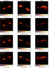 |
Fig. 2 Gaussian convolved model images of Cygnus A, Hydra A, Hercules A, and M106 (upper row), and their respective reconstructions with the VLA in A configuration with CLEAN (second row), with Asp-CLEAN (third row), and with Autocorr-CLEAN (fourth row). |
4.3 Quantitative assessment of imaging performance
Finally, we discuss the convergence speed of the algorithms. In Fig. 4, we show the recovered model and residual as a function of iteration and computational time. The same plots for M106 and Hercules A are shown in Appendix A. In Fig. 5, we show a more quantitative assessment of the convergence speed. To study the convergence speed, we make use of the fact that we know the ground truth image in these tests. While typically the residual is used as a measure for the precision of an algorithm, this quantity only estimates the quality of the fit to the incompletely sampled visibilities. Here, we evaluate the norm difference between the truth and the reconstruction instead. However, this distance in linear scale may be dominated by the reconstruction fidelity of a few pixels describing compact emission, such as the shocks in the Cygnus A example. Therefore, in Fig. A.4, we also show the difference between the logarithms of the ground truth and the reconstruction for Cygnus A.
In terms of number of iterations, both Asp-CLEAN and Autocorr-CLEAN converge much faster than CLEAN. This is not a surprise though. In Autocorr-CLEAN we fit multiple CLEAN components at once in every minor loop iteration. The number of minor loop iterations that are needed for Autocorr-CLEAN is traded for the number of iterations that are spent in the subminor loop.
The convergence as a function of computational time is therefore a fairer comparison. This one is shown in the bottom panels in Fig. 5. To perform a fair comparison of the algorithms alone free of effects stemming from the architecture and respective implementation, we reimplemented CLEAN in LibRA in C++ (rather than the Fortran binding called internally) with the same code-block structures that were also used for the implementation for Autocorr-CLEAN, Asp-CLEAN, and MS-CLEAN. Moreover, we ran both algorithms on the same computational infrastructure with a CPU of 16 cores that, at the time of performing the benchmarks, was cleared of any other process running on the system.
Autocorr-CLEAN performs significantly faster in terms of time than CLEAN. This stems from two important features. First, there are typically fewer iterations performed in the subminor loop than the number of components in the basis function co. Hence, we gain more by fitting multiple components at once than we spend on finding these components. Second, the majority of the update steps of the quantities MI, BI, MBI,... in the subminor loop and the minor loop can be effectively parallelized.
Finally, the speedup of Autocorr-CLEAN in contrast to Asp-CLEAN is quite significant. Asp-CLEAN computes a model fitting step at every iteration, adapting a Gaussian to the current residual. Particularly, the repeated evaluation of the Fourier transform slows the algorithm down (Hsieh & Bhatnagar 2021). Asp-CLEAN is faster than Autocorr-CLEAN in all four examples on the first iteration only, since the head-on processing for Autocorr-CLEAN is bigger (i.e., the initialization of the autocorrelation products and the first approximation of co; block 3 in Algorithm 1). However, after only a few iterations Autocorr-CLEAN already overtakes Asp-CLEAN in convergence speed since the evaluation of a few subminor loop iterations is much faster than the update step for Asp-CLEAN. We do note however that Asp-CLEAN seems to allow deeper CLEANing of the diffuse emission as indicated by the difference to the ground truth in logarithmic scale.
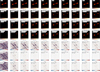 |
Fig. 4 Recovered model and respective residual for different deconvolution techniques as a function of number of iterations. Upper panels: Gaussian convolved model as a function of number of iterations. Lower panels: Residual as a function of number of iterations. |
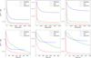 |
Fig. 5 Speed of convergence for the different techniques as a function of number of iterations (top row) and computational time (bottom row). Left column: Cygnus A, middle column: Hercules A, right column: M106. |
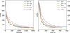 |
Fig. 6 Convergence curves for Autocorr-CLEAN with different values of y for the Cygnus A example. |
4.4 Control parameters
We discuss multiple control parameters in Sect. 3.3, particularly the stopping criterion for the subminor loop determined by the relative fraction f, and the power parameter γ. We provided some natural motivation and choices in Sect. 3.3. In this section, we present some evaluation on synthetic data.
Figure 6 shows the convergence curve for Autocorr-CLEAN for the Cygnus A synthetic data set for varying power parameters γ. We recall that a Gaussian approximation would hold the value γ = 2. We find the fastest convergence in terms of number of minor loop iterations and computational time for values γ = 1.5 and γ = 2. However, we note that even for parameter choices outside of the range of preferred values (e.g., γ = 1 or γ = 3), we observe a quite favorable convergence curve outperforming Asp-CLEAN and CLEAN.
The fraction parameter f determines the number of subminor loop iterations. We show the convergence curve for varying fractional parameters f in Fig. 7. The smaller the value of f, the greater the number of subminor loop iterations executed. This is observed to help the convergence in the first iterations when diffuse extended emission is present in the image; for example, large-scale basis functions need to be deployed. In contrast, for small values of f we spend more time in the subminor loop, potentially slowing the algorithm down. Moreover, we have observed that when f is smaller, the algorithm switches to the point-source dominated Hogbom CLEAN scheme more quickly. This is well explained by the fact that the extended diffuse emission is going to be removed with fewer minor loop iterations. Overall, we observe a quicker convergence for more generous fractions as long as the fraction f is small enough to force the algorithm to fit a correlated model rather than point components (which is effectively CLEAN).
One significant advantage of Asp-CLEAN is its robustness against the CLEAN gain. While traditional CLEAN diverges for big gains, Asp-CLEAN allows using a bigger CLEAN gain (Bhatnagar & Cornwell 2004). This is because of the adaptive scale adaptation performed in every minor loop iteration, and may have significant impact on the convergence speed as a function of time. For the comparison in Sect. 4.3, we used the same CLEAN gain for every approach to assess the convergence speed in a fair same-level comparison. Here, we test increasing gains. The residuals for Autocorr-CLEAN and Asp-CLEAN as a function of number of iteration for Cygnus A, for gains ranging between 0.1 and 0.5 are shown in Fig. A.5. We note that in comparison to Fig. 4, we adapted the colorbar of the residual since the shown algorithms converge faster than CLEAN did. We can observe that for Asp-CLEAN the residual is cleaned faster with higher gains, although when inspecting the clock times, still slower than Autocorr-CLEAN. Autocorr-CLEAN performs faster for a gain of 0.3, but the accumulation of errors at even higher CLEAN gains (i.e., 0.5) worsens the model again.
Finally, it should be noted that we achieved the fastest performance for relatively aggressive values for f and the gain. While this may be expected in the image-plane scenario discussed in this manuscript, the best-performing values may be too aggressive in the presence of gridding and calibration errors or requires a relatively high dynamic range between large-scale structures and other structures.
5 Conclusion
In this manuscript, we presented a novel multiscalar CLEAN variant, named Autocorr-CLEAN. Autocorr-CLEAN draws strong inspiration from MS-CLEAN algorithms that were proposed in the past (i.e., the clustering of components in a subminor loop (Offringa & Smirnov 2017)), continuously varying multiscale components (Bhatnagar & Cornwell 2004), and potentially non-radially symmetric basis functions (Müller & Lobanov 2023b). The Autocorr-CLEAN minor loop consists of a scheme switching between a MS-CLEAN step performed on the residual with a cluster of CLEAN components, and subminor loop at which this cluster of CLEAN components is adapted to the autocorrelation function of the residual.
The implementation of every single step is fast thanks to the avoidance of any step of super-linear numerical complexity (i.e., only shifting of arrays, and additions or substitutions), and the great potential to perform the update steps in a parallel fashion. The convergence speed of Autocorr-CLEAN in terms of number of iterations matches the performance of Asp-CLEAN, one of the most advanced, but also most computationally demanding multi-scalar CLEAN approaches. This is caused by the extensive fitting of multiple components all at once in every single minor loop iteration. Combining these two properties, fast numerical execution of every single minor loop iteration and enhanced numerical convergence speed, Autocorr-CLEAN significantly outperforms classical CLEAN approaches and its many variants.
We benchmarked the performance of Autocorr-CLEAN in synthetic data sets mimicking an observation with the VLA in A configuration. We observed that Autocorr-CLEAN reduces the residual to the same level as ordinary CLEAN in five to ten times less time, and goes on to recover even fainter features. The quality of the reconstruction matches state-of-the-art MS-CLEAN reconstructions, even outperforming them for very wide diffuse emission, and significantly outperforming plain CLEAN at all spatial scales. This is caused by the superior localization of the model components when fitting a correlated signal compared to the point-source-based CLEAN algorithm. However, the main benefit of Autocorr-CLEAN is its speed and it ability to achieve these depths at low numerical cost.
In this manuscript, we limited ourself to a proof of concept. A full evaluation of the performance of the algorithm covering a variety of observational setups is beyond the scope of this work, and may only be delivered by gathering practical experience over time, as was done for CLEAN. We would like to note, however, that because Autocorr-CLEAN was developed and implemented in the widely used CASA environment, and because it is based on relatively solid and well proven strategies for radio inter-ferometry, it may reduce the barrier to applications in practice that currently exist for many novel approaches to imaging and calibration.
In this manuscript, we only dealt with the minor loop; we studied an image-plane problem only. Consecutive works and practical experience need to determine the mutual impact of Autocorr-CLEAN on the gridding, flagging, and calibration. A particular area where practical experience is needed is the relative tradeoff between the accuracy of the approximation of the auto-correlation structure and the CLEANing of the residual itself. In this work we evaluated the impact of several choices, and concluded with naturally motivated recommendations, which however could prove to be too aggressive in a low dynamic range or less accurately calibrated situations.
Due to its design with deep roots in the classical hierarchy of algorithms commonly used for aperture synthesis, we expect Autocorr-CLEAN to work well together with the recent algorithmic improvements that were demonstrated to boost the dynamic range of the recovered image. That includes, among others, various modern projection algorithms to deal with wide-field and wide-band effects (e.g., Bhatnagar & Cornwell 2017) or the iterative refinement technique based on multiscalar masks presented in Offringa & Smirnov (2017).
In conclusion, Autocorr-CLEAN may be a useful asset in the much needed attempt to scale up current routines in radio interferometry to the data sizes that are expected from the next generation of high precision radio interferometers, such as the SKA, ngVLA, or ALMA operations after the wide-band sensitivity upgrade. It ideally complements a variety of developments to scale up the remaining parts of the data reduction pipeline (e.g., gridding or radio frequency mitigation) as well.
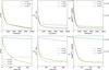 |
Fig. 7 Convergence curves for Autocorr-CLEAN with different values of f for the Cygnus A example. |
Acknowledgements
We thank Rick Perley for providing the data sets used in this manuscript. The analysis was performed with the software tool LibRA3. H.M. wants to thank Prashanth Jagannathan and Mingyu Hsieh for critical support in setting up this library for this work. This research was supported through the Jan-sky fellowship program of the National Radio Astronomy Observatory. NRAO is a facility of the National Science Foundation operated under cooperative agreement by Associated Universities, Inc.. Furthermore, H.M. acknowledges support by the M2FINDERS project which has received funding from the European Research Council (ERC) under the European Union's Horizon 2020 Research and Innovation Program (grant agreement No. 101018682).
Appendix A Supplementary figures
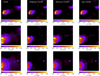 |
Fig. A.1 Zoomed-in view of the reconstruction of Cygnus A, highlighting the improved reconstruction features at small scales. |
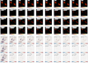 |
Fig. A.2 Same as Fig. 4, but for Hercules A. Upper panels: Gaussian convolved model as a function of number of iterations. Lower panels: Residual as a function of number of iterations. |
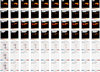 |
Fig. A.3 Same as Fig. 4, but for M106. Upper panels: Gaussian convolved model as a function of number of iterations. Lower panels: Residual as a function of number of iterations. |
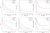 |
Fig. A.4 Convergence of the reconstruction for Cygnus A for different metrics: norm of the residual (left panels), distance to the ground truth (middle panels), and distance of the logarithms of the true and recovered features (right panels). The upper panels present the reconstructions as a function of number of iterations, the lower panels as a function of computational time. |
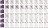 |
Fig. A.5 Residuals for Cygnus A with Autocorr-CLEAN (rows 1, 3, and 5) and Asp-CLEAN (rows 2,4, and 6) with varying gains a function of number of iterations. |
References
- Aghabiglou, A., Chu, C. S., Dabbech, A., & Wiaux, Y. 2024, ApJS, 273, 3 [NASA ADS] [CrossRef] [Google Scholar]
- Arras, P., Bester, H. L., Perley, R. A., et al. 2021, A&A, 646, A84 [NASA ADS] [CrossRef] [EDP Sciences] [Google Scholar]
- Bhatnagar, S., & Cornwell, T. J. 2004, A&A, 426, 747 [NASA ADS] [CrossRef] [EDP Sciences] [Google Scholar]
- Bhatnagar, S., & Cornwell, T. J. 2017, AJ, 154, 197 [Google Scholar]
- Bhatnagar, S., Cornwell, T. J., Golap, K., & Uson, J. M. 2008, A&A, 487, 419 [NASA ADS] [CrossRef] [EDP Sciences] [Google Scholar]
- Bhatnagar, S., Rau, U., & Golap, K. 2013, ApJ, 770, 91 [Google Scholar]
- Bhatnagar, S., Hirart, R., & Pokorny, M. 2021, Size-of-Computing Estimates for ngVLA Synthesis Imaging, NRAO-The ngVLA Memo Series: Computing Memos [Google Scholar]
- Bhatnagar, S., Madsen, F., & Robnett, J. 2022, Baseline HPG runtime performance for imaging, NRAO-The ngVLA Memo Series: Computing Memos [Google Scholar]
- Carrillo, R. E., McEwen, J. D., & Wiaux, Y. 2012, MNRAS, 426, 1223 [Google Scholar]
- CASA Team (Bean, B., et al.) 2022, PASP, 134, 114501 [NASA ADS] [CrossRef] [Google Scholar]
- Clark, B. G. 1980, A&A, 89, 377 [NASA ADS] [Google Scholar]
- Cornwell, T. J. 2008, IEEE J. Selected Top. Signal Process., 2, 793 [NASA ADS] [CrossRef] [Google Scholar]
- Dabbech, A., Repetti, A., Perley, R. A., Smirnov, O. M., & Wiaux, Y. 2021, MNRAS, 506, 4855 [NASA ADS] [CrossRef] [Google Scholar]
- Dabbech, A., Aghabiglou, A., Chu, C. S., & Wiaux, Y. 2024, ApJ, 966, L34 [NASA ADS] [CrossRef] [Google Scholar]
- Event Horizon Telescope Collaboration (Akiyama, K., et al.) 2024, ApJ, 964, L25 [NASA ADS] [CrossRef] [Google Scholar]
- Gao, A. F., Leong, O., Sun, H., & Bouman, K. L. 2023, in ICASSP 2023-2023 IEEE International Conference on Acoustics, Speech and Signal Processing (ICASSP), IEEE, 1 [Google Scholar]
- Högbom, J. A. 1974, A&AS, 15, 417 [Google Scholar]
- Homan, D. C., Roth, J. S., & Pushkarev, A. B. 2024, AJ, 167, 11 [Google Scholar]
- Hsieh, G., & Bhatnagar, S. 2021, Efficient Adaptive-Scale CLEAN Deconvolution in CASA for Radio Interferometric Images, NRAO-ARDG Memo Series [Google Scholar]
- Hsieh, G., Bhatnagar, S., Hiriart, R., & Pokorny, M. 2022a, Recommended Developments Necessary for Applying (W)Asp Deconvolution Algorithms to ngVLA, NRAO-ARDG Memo Series [Google Scholar]
- Hsieh, G., Rau, U., & Bhatnagar. 2022b, An Adaptive-Scale Multi-Frequency Deconvolution of Interferometric Images, NRAO-ARDG Memo Series [Google Scholar]
- Jarret, A., Kashani, S., Rué-Queralt, J., et al. 2025, A&A, 693, A225 [NASA ADS] [CrossRef] [EDP Sciences] [Google Scholar]
- Junklewitz, H., Bell, M. R., Selig, M., & Enßlin, T. A. 2016, A&A, 586, A76 [NASA ADS] [CrossRef] [EDP Sciences] [Google Scholar]
- Kashani, S., Rué Queralt, J., Jarret, A., & Simeoni, M. 2023, arXiv e-prints [arXiv:2306.06007] [Google Scholar]
- Kepley, A. A., Tsutsumi, T., Brogan, C. L., et al. 2020, PASP, 132, 024505 [Google Scholar]
- Kepley, A., Madsen, F., Robnet, J., & Rowe, K. 2023, Imaging Unmitigated ALMA Cubes, NRAO-NAASC memo series [Google Scholar]
- Kim, J.-S., Mueller, H., Nikonov, A. S., et al. 2025, A&A, 696, A169 [NASA ADS] [CrossRef] [EDP Sciences] [Google Scholar]
- Kramer, J. A., Müller, H., Röder, J., & Ros, E. 2025, A&A, 697, A66 [NASA ADS] [CrossRef] [EDP Sciences] [Google Scholar]
- Lannes, A., Anterrieu, E., & Marechal, P. 1997, A&AS, 123, 183 [NASA ADS] [CrossRef] [EDP Sciences] [Google Scholar]
- McMullin, J. P., Waters, B., Schiebel, D., Young, W., & Golap, K. 2007, in Astronomical Society of the Pacific Conference Series, 376, Astronomical Data Analysis Software and Systems XVI, eds. R. A. Shaw, F. Hill, & D. J. Bell, 127 [NASA ADS] [Google Scholar]
- Müller, H. 2024, A&A, 689, A299 [NASA ADS] [CrossRef] [EDP Sciences] [Google Scholar]
- Müller, H., & Lobanov, A. P. 2022, A&A, 666, A137 [NASA ADS] [CrossRef] [EDP Sciences] [Google Scholar]
- Müller, H., & Lobanov, A. P. 2023a, A&A, 673, A151 [NASA ADS] [CrossRef] [EDP Sciences] [Google Scholar]
- Müller, H., & Lobanov, A. P. 2023b, A&A, 672, A26 [NASA ADS] [CrossRef] [EDP Sciences] [Google Scholar]
- Müller, H., Mus, A., & Lobanov, A. 2023, A&A, 675, A60 [NASA ADS] [CrossRef] [EDP Sciences] [Google Scholar]
- Müller, H., Massa, P., Mus, A., Kim, J.-S., & Perracchione, E. 2024, A&A, 684, A47 [NASA ADS] [CrossRef] [EDP Sciences] [Google Scholar]
- Mus, A., Müller, H., & Lobanov, A. 2024a, A&A, 688, A100 [NASA ADS] [CrossRef] [EDP Sciences] [Google Scholar]
- Mus, A., Müller, H., Martí-Vidal, I., & Lobanov, A. 2024b, A&A, 684, A55 [NASA ADS] [CrossRef] [EDP Sciences] [Google Scholar]
- Offringa, A. R., & Smirnov, O. 2017, MNRAS, 471, 301 [Google Scholar]
- Offringa, A. R., McKinley, B., Hurley-Walker, N., et al. 2014, MNRAS, 444, 606 [Google Scholar]
- Onose, A., Carrillo, R. E., Repetti, A., et al. 2016, MNRAS, 462, 4314 [NASA ADS] [CrossRef] [Google Scholar]
- Onose, A., Dabbech, A., & Wiaux, Y. 2017, MNRAS, 469, 938 [NASA ADS] [CrossRef] [Google Scholar]
- Paraschos, G. F., Debbrecht, L. C., Kramer, J. A., et al. 2024, A&A, 686, L5 [NASA ADS] [CrossRef] [EDP Sciences] [Google Scholar]
- Rau, U., & Cornwell, T. J. 2011, A&A, 532, A71 [NASA ADS] [CrossRef] [EDP Sciences] [Google Scholar]
- Roelofs, F., Blackburn, L., Lindahl, G., et al. 2023, Galaxies, 11, 12 [NASA ADS] [CrossRef] [Google Scholar]
- Roth, J., Arras, P., Reinecke, M., et al. 2023, A&A, 678, A177 [NASA ADS] [CrossRef] [EDP Sciences] [Google Scholar]
- Schmidt, K., Geyer, F., Fröse, S., et al. 2022, A&A, 664, A134 [NASA ADS] [CrossRef] [EDP Sciences] [Google Scholar]
- Schwab, F. R. 1984, AJ, 89, 1076 [NASA ADS] [CrossRef] [Google Scholar]
- Starck, J. L., & Murtagh, F. 2006, Astronomical Image and Data Analysis (Springer) [CrossRef] [Google Scholar]
- Starck, J.-L., Bijaoui, A., Lopez, B., & Perrier, C. 1994, A&A, 283, 349 [NASA ADS] [Google Scholar]
- Starck, J.-L., Candes, E. J., & Donoho, D. L. 2002, IEEE Trans. Image Process., 11, 670 [CrossRef] [Google Scholar]
- Starck, J. L., Elad, M., & Donoho, D. L. 2005, IEEE Trans. Image Process., 14, 1570 [Google Scholar]
- Starck, J.-L., Murtagh, F., & Fadili, J. 2015, Sparse Image and Signal Processing: Wavelets and Related Geometric Multiscale Analysis, 2nd edn., 1 [Google Scholar]
- Tasse, C., van der Tol, S., van Zwieten, J., van Diepen, G., & Bhatnagar, S. 2013, A&A, 553, A105 [NASA ADS] [CrossRef] [EDP Sciences] [Google Scholar]
- Thompson, A. R., Moran, J. M., & Swenson, George W. J. 2017, Interferometry and Synthesis in Radio Astronomy, 3rd edn. (Springer) [CrossRef] [Google Scholar]
- Wakker, B. P., & Schwarz, U. J. 1988, A&A, 200, 312 [NASA ADS] [Google Scholar]
- Wiaux, Y., Jacques, L., Puy, G., Scaife, A. M. M., & Vandergheynst, P. 2009, MNRAS, 395, 1733 [NASA ADS] [CrossRef] [Google Scholar]
- Zhang, L., Bhatnagar, S., Rau, U., & Zhang, M. 2016, A&A, 592, A128 [NASA ADS] [CrossRef] [EDP Sciences] [Google Scholar]
Retrieved from https://chandra.harvard.edu/photo/openFITS/multiwavelength_data.html
All Figures
|
Fig. 1 Autocorrelation of the initial residual ( |
| In the text | |
|
Fig. 2 Gaussian convolved model images of Cygnus A, Hydra A, Hercules A, and M106 (upper row), and their respective reconstructions with the VLA in A configuration with CLEAN (second row), with Asp-CLEAN (third row), and with Autocorr-CLEAN (fourth row). |
| In the text | |
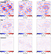 |
Fig. 3 Residual images for the reconstructions shown in Fig. 2. |
| In the text | |
|
Fig. 4 Recovered model and respective residual for different deconvolution techniques as a function of number of iterations. Upper panels: Gaussian convolved model as a function of number of iterations. Lower panels: Residual as a function of number of iterations. |
| In the text | |
|
Fig. 5 Speed of convergence for the different techniques as a function of number of iterations (top row) and computational time (bottom row). Left column: Cygnus A, middle column: Hercules A, right column: M106. |
| In the text | |
|
Fig. 6 Convergence curves for Autocorr-CLEAN with different values of y for the Cygnus A example. |
| In the text | |
|
Fig. 7 Convergence curves for Autocorr-CLEAN with different values of f for the Cygnus A example. |
| In the text | |
|
Fig. A.1 Zoomed-in view of the reconstruction of Cygnus A, highlighting the improved reconstruction features at small scales. |
| In the text | |
|
Fig. A.2 Same as Fig. 4, but for Hercules A. Upper panels: Gaussian convolved model as a function of number of iterations. Lower panels: Residual as a function of number of iterations. |
| In the text | |
|
Fig. A.3 Same as Fig. 4, but for M106. Upper panels: Gaussian convolved model as a function of number of iterations. Lower panels: Residual as a function of number of iterations. |
| In the text | |
|
Fig. A.4 Convergence of the reconstruction for Cygnus A for different metrics: norm of the residual (left panels), distance to the ground truth (middle panels), and distance of the logarithms of the true and recovered features (right panels). The upper panels present the reconstructions as a function of number of iterations, the lower panels as a function of computational time. |
| In the text | |
|
Fig. A.5 Residuals for Cygnus A with Autocorr-CLEAN (rows 1, 3, and 5) and Asp-CLEAN (rows 2,4, and 6) with varying gains a function of number of iterations. |
| In the text | |
Current usage metrics show cumulative count of Article Views (full-text article views including HTML views, PDF and ePub downloads, according to the available data) and Abstracts Views on Vision4Press platform.
Data correspond to usage on the plateform after 2015. The current usage metrics is available 48-96 hours after online publication and is updated daily on week days.
Initial download of the metrics may take a while.