| Issue |
A&A
Volume 698, June 2025
|
|
|---|---|---|
| Article Number | A76 | |
| Number of page(s) | 15 | |
| Section | Planets, planetary systems, and small bodies | |
| DOI | https://doi.org/10.1051/0004-6361/202452016 | |
| Published online | 29 May 2025 | |
Inferring the interior oxygen fugacity of rocky exoplanets from observations: Assessing biases by atmospheric chemistry
1
University of Paris Saclay, OVSQ, LATMOS,
11 Boulevard d’Alembert,
78280
Guyancourt,
France
2
Ludwig Maximilian University, Faculty of Physics, Observatory of Munich,
Scheinerstrasse 1,
Munich
81679,
Germany
3
ENS Paris-Saclay,
4 avenue des Sciences,
91190
Gif-sur-Yvette,
France
4
University of Bern, ARTORG Center for Biomedical Engineering Research,
Murtenstrasse 50,
3008,
Bern,
Switzerland
5
University College London, Department of Physics & Astronomy,
Gower St,
London
WC1E 6BT,
UK
6
University of Warwick, Department of Physics, Astronomy & Astrophysics Group,
Coventry
CV4 7AL,
UK
★ Corresponding author: This email address is being protected from spambots. You need JavaScript enabled to view it.
Received:
27
August
2024
Accepted:
24
February
2025
Abstract
In the era of the James Webb Space Telescope, inferring the presence and bulk composition of temperate rocky exoplanet atmospheres is now possible. The primary targets typically have equilibrium temperatures ranging from 400 to 1500 K, for which a balance between geochemical outgassing and escape is required to maintain an atmosphere. The composition of these exoplanet atmospheres hold crucial information on the redox state of the planetary interior characterized by the oxygen fugacity (fo2). The relative molecular abundances of volatile species with opposite redox states inferred from observations can help constrain an effective interior fo2. Using different model complexities from 0D simulations of chemical equilibrium to 1D atmospheric simulations with outgassing and self-consistent iterations of atmospheric chemistry (photochemistry and thermochemistry) and radiative transfer, we assess the reliability of using relative abundances in a C−H−O system to infer fo2. The CO2/CO, previously suggested as the most reliable tracer of fo2, is increased by atmospheric cooling (thermochemical cooling between melt and atmosphere) and photochemistry, which would cause a bias of approximately one to two orders of magnitude on the retrieved fo2. Constraints on the atmospheric temperature can help correct the effect of atmospheric cooling and improve the retrieval of fo2. The increase of CO2/CO driven by photochemistry is dominant for thin atmospheres, although it occurs over long timescales (tens or hundreds of thousands of years) and therefore would be negligible if the atmosphere is continuously replenished by outgassing. The transition between a chemical regime dominated by atmospheric thermochemistry toward a regime dominated by photochemistry is controlled not only by surface pressure and temperature but also by oxygen fugacity itself (via O/H). Inferring CO2/CO from the data might be challenging given the low contribution of CO in transit and emission spectra for objects with high CO2 and H2O abundances. We suggest CO2/CH4 as an alternative tracer of fo2, although high methane abundances are only expected in reducing conditions (i.e., less than the iron–wustite buffer) and high pressure-temperature surface conditions favoring the buildup of CH4 by atmospheric cooling.
Key words: planets and satellites: atmospheres / planets and satellites: detection / planets and satellites: terrestrial planets
© The Authors 2025
 Open Access article, published by EDP Sciences, under the terms of the Creative Commons Attribution License (https://creativecommons.org/licenses/by/4.0), which permits unrestricted use, distribution, and reproduction in any medium, provided the original work is properly cited.
This article is published in open access under the Subscribe to Open model. This email address is being protected from spambots. You need JavaScript enabled to view it. to support open access publication.
1 Introduction
The NASA Kepler mission dedicated to the search for exoplanets (Borucki et al. 2010) revealed that objects with radii smaller than Neptune are the most abundant in the galaxy, making up more than three-fourths of the entire population (Borucki et al. 2011; Batalha et al. 2013). The distribution of exoplanet radii measured with Kepler exhibits a gap at ≈ 1.5 R⊕ (Fulton et al. 2017), referred to in the literature as the “radius gap,” that marks the transition between the categories of super-Earth (Rp < 1.5 R⊕) and sub-Neptune (Rp > 1.5 R⊕). The latter objects are likely composed of a rocky core surrounded by a H2-He primitive envelope that survived erosion during the early active phase of the star, whereas the former lost this light primitive atmosphere through extreme ultraviolet (XUV) stellar heating (i.e., photo-evaporation) and/or the transfer of energy from a cooling interior (i.e., core-powered mass loss) (Owen & Wu 2013; Lopez & Fortney 2013; Fulton & Petigura 2018; Loyd et al. 2020; Van Eylen et al. 2018; MacDonald 2019; Gupta & Schlichting 2019).
The dominant mass-loss mechanism shaping the radius valley remains debated in the literature; both photo-evaporation and core-powered mass-loss can play a crucial role at different stages in the planet’s evolution (Owen & Schlichting 2024). With this primitive envelope lost, planets with sizes below the radius gap could host secondary atmospheres produced via outgassing, similarly to the rocky planets in the inner Solar System (Gaillard & Scaillet 2014; Gillmann et al. 2024).
For rocky exoplanets below the radius gap, a broad range of bulk densities have been reported, suggesting variations from water worlds to Earth-like silicate-rich objects to Fe-rich super-Mercuries (Weiss & Marcy 2014; Luque & Pallé 2022). The variety of metallicities observed in the host stars (Buchhave et al. 2012; Brewer & Fischer 2016) further supports the expected diversity in interior composition. Planetary mass and radius (M-R) measurements have provided crucial first insights into the internal structure, suggesting that a large fraction of rocky exoplanets have a massive core (Dorn et al. 2015; Liu & Ni 2023; Unterborn et al. 2023). Although the core to mantle fraction can be well constrained with M-R measurements, the degeneracy on the mantle composition is substantial (Seager et al. 2007) and can only be solved if the relative abundances of refractories from the star are known (Dorn et al. 2015; Unterborn et al. 2016). This approach assumes a comparable composition between star and planet, a reasonable and validated starting hypothesis (Thiabaud et al. 2015), with some exceptions where planet formation mechanisms could modify the correlation (Adibekyan et al. 2021; Schulze et al. 2021).
The rocky interior properties, including volatile budget and redox state, control the composition of the surrounding secondary atmosphere (Gaillard et al. 2021). The speciation of gas species is primarily controlled by the interior redox state quantified with the oxygen fugacity (fo2), a key parameter reflecting the relative abundance of ferric iron relative to the total iron content (Fe3+/ΣFe) in the melt, with high fo2 favoring the oxidation of ferrous iron in the buffer reaction FeO +  O2 ⟷ FeO3/2 or the oxidation of metallic iron in the buffer reaction Fe +
  O2 ⟷ FeO (Frost & McCammon 2008; Burgisser et al. 2015; Sossi et al. 2020; Deng et al. 2020; Ortenzi et al. 2020; Liggins et al. 2022; Guimond et al. 2023). This latter buffer reaction, called the iron-wustite (IW) buffer, is often used to express the fo2 relative to a reference (e.g., Tian & Heng 2024). The melt oxygen fugacity is controlled by pressure (Deng et al. 2020) as well as (volatile) composition (Young et al. 2023).
For ultra-short-period (USP) exoplanets, the high surface temperature forced by incoming stellar radiation should favor the formation of a sustained magma ocean in these so-called “lava worlds.” In this scenario, the atmosphere is directly at equilibrium with the upper layers of the magma ocean, and the characterization of the gas composition can provide crucial information on the interior properties (Gaillard et al. 2021, 2022). Several models have been developed to describe the composition of the atmosphere at equilibrium with the magma ocean accounting for the solubility of volatile species in silicate melts (Sossi et al. 2020; Gaillard et al. 2022; Liggins et al. 2022; Bower et al. 2022; Wolf et al. 2023). A large diversity of atmospheric compositions can be produced depending on the fo2, from CO- to H2- to CO2-dominated atmospheres (Gaillard et al. 2022; Tian & Heng 2024). However, steam atmospheres are less likely given the high solubility of water in silicate melts (Bower et al. 2022; Sossi et al. 2023). Based on the strong correlation between the fo2 of the magma and the atmospheric composition, it has been suggested that specific relative abundances of volatiles in the atmosphere can help constrain the oxygen fugacity of the interior, with CO2/CO being the most robust candidate (Tian & Heng 2024; Shorttle et al. 2024). Beyond volatiles, the atmospheres of lava worlds can contain significant amounts of vaporized refractories including silicate and magnesium oxides, which can also help constrain the interior redox state (Wolf et al. 2023; Seidler et al. 2024).
For secondary atmospheres of cooler planets with a crystallized crust, the mass and composition of the atmosphere result from a balance between volcanic degassing and atmospheric escape (Ortenzi et al. 2020; Liggins et al. 2020). The degassing rate is mainly controlled by planet mass and internal heating, the latter being controlled via tidal or radiogenic processes that allow partial melting in the upper mantle (Dorn et al. 2018; Quick et al. 2020; Oosterloo et al. 2021). For Mp < 2−3 M⊕, the degassing rate increases with planet mass, making secondary atmospheres around massive super-Earths more likely (Dorn et al. 2018) unless the convection efficiency is reduced by a higher core fraction (Oosterloo et al. 2021). In simplified models, the degassing rate is derived using the mantle melt fraction, rock-melt partition coefficients, and the approximated mantle convection rate (Ortenzi et al. 2020; Liggins et al. 2022). The process of degassing is thus subjected to too many unknown variables, although the outgassed composition is mainly controlled by the volatile budget and the oxygen fugacity (fo2) in a manner similar to a magma ocean scenario (Gaillard & Scaillet 2014; Liggins et al. 2020, 2022; Tian & Heng 2024). Although the planetary size is a key parameter controlling the interior fo2, variations in the mantle mineralogy can also modify fo2 by orders of magnitude (Guimond et al. 2023). In other words, the large diversity in planetary mass-radius and composition (refractories) observed in the exoplanet population will likely produce rocky exoplanet atmospheres with a variety of compositions. Contrary to a magma ocean scenario, a difference in temperature is expected between the melt and the surface of the planet. This process where the warm degassed volatiles cool in a new atmospheric environment, which we refer to as atmospheric cooling, can modify the composition of the atmosphere and thus affect observations (Liggins et al. 2023). Other processes affecting the composition of the upper atmosphere probed during spectroscopic observations, such as escape and photochemistry, can modify the degassed composition (Liggins et al. 2020; Krissansen-Totton & Fortney 2022) and thus bias our objective, which is focused on inferring properties of the rocky interior.
The atmospheric composition and relative abundances of volatile species with different redox states is first set by geochemical outgassing but modified by atmospheric chemistry (photochemistry and thermochemistry). In the present study, we focus on secondary atmospheres of evolved planetary bodies with a crystallized crust and assess the biases caused by photochemistry and atmospheric cooling as well as their influence on future atmospheric characterization in order to constrain the interior fo2. In Sect. 2, we present the models we used and the simulations performed for this study considering geochemical outgassing with self-consistent calculations of atmospheric chemistry and radiative transfer. In Sect. 3, we describe the effect of atmospheric cooling (thermochemistry) on relative molecular abundances used as tracers of the interior fo2. In Sect. 4, we assess the effect of atmospheric cooling, photochemistry, and vertical mixing on the relative abundances for a 1D case study of the super-Earth GJ 1132b. In Sect. 5, we discuss the implications for future observations with the James Webb Space Telescope (JWST).
2 Model description
2.1 Outgassing model: C–H–O gas at equilibrium with carbon-bearing melt
The outgassing model used for this study is described in detail in Tian & Heng (2024) following an approach initially introduced by French (1966). The model assumes chemical equilibrium between a C-H-O fluid phase and a carbon-bearing melt. At the pressures considered in this study (below 100 bars), ideal gas may be assumed (Tian & Heng 2024) which simplifies the determination of the gas partial pressures to an analytical calculation. Only four parameters are needed to determine the speciation of the gas at equilibrium with the carbon-bearing melt: oxygen fugacity, activity of graphite (Ac), melt temperature (Tm) and degassing pressure (Pd). The chemical system can be described by a set of four independent reactions:
 (R1)
(R1)
 (R2)
(R2)
 (R3)
(R3)
 (R4)
(R4)
The IW buffer is expressed following Ballhaus et al. (1991) based on the experimental data of O’Neill (1987). The current model does not consider solubility, and it thus does not require volatile inventories as an input parameter unlike other models applying mass balance (e.g., Gaillard & Scaillet 2014 or Liggins et al. 2020). In practice, it means that the total gas pressure is set in our model and not calculated considering the solubility of each gaseous species in the melt. We emphasize that the lack of solubility in the model does not bias the correlation between CO2/CO and fo2 reflected with reactions (R1) and (R2). CO2/CO remains directly correlated to fo2 following XCO2/XCO = fo20.5/Keq, with X the molecular abundance and Keq the equilibrium constant of the reaction CO + 0.5 O2 ⟷ CO2 (i.e., (R1)–(R2)). Although the model of Tian & Heng (2024) can consider N- and S-bearing species, these will not be considered in the present work since our approach targets molecular abundances that can directly inform on the interior redox state such as CO2/CO. Speciation between N2 and NH3 is controlled by the amount of H2 in the system which will be difficult to constrain with atmospheric characterization. In addition, the solubility of ammonia in the melt, which is not considered here, can be important to explain the abundances found in the atmosphere (Shorttle et al. 2024). Molecular abundances of sulfur-bearing compounds are also highly sensitive to solubility, even at low pressures.
In our calculations, Tm is set to 1600 K, a typical melt temperature used in previous studies (Gaillard & Scaillet 2014; Gaillard et al. 2022). Degassing is assumed to occur under atmospheric pressure (i.e., Pd = Ps) similar to the approach of Gaillard & Scaillet (2014).
2.2 OD calculations of atmospheric cooling
Rocky exoplanets currently observed with JWST exhibit different masses and radii (Luque & Pallé 2022) with likely different interior compositions (suggested by stellar observations) that would create different atmospheric compositions. To avoid the large number of unknowns required to compute outgassing and escape fluxes, we consider a state where both processes balance using a parametrized surface pressure. In other words, the outgassing model is used to set the initial composition of the atmosphere at a given pressure, we do not consider a continuous volcanic flux at the surface. Boundary conditions including surface deposition and escape are not considered as we focus on the effect of atmospheric chemistry. Most rocky exoplanets observed with JWST present equilibrium temperatures between 400 K and 1500 K. If these objects maintained an atmosphere, the volatiles outgassed from the interior will cool to the new temperature found in the atmosphere. This atmospheric cooling mechanism will modify the stable gas abundances according to the new pressure-temperature conditions found in the atmosphere (Liggins et al. 2023).
After atmospheric cooling, the molecular abundances might change significantly compared to the prediction of the outgassing model. To assess the change in molecular abundances of a volcanic mixture subjected to atmospheric cooling, we combine the geochemical outgassing calculations of Tian & Heng (2024) with atmospheric thermochemical calculations performed using FastChem and VULCAN. FastChem, described in detail in Stock et al. (2018) and Stock et al. (2022), uses a semi-analytical approach to determine the molecular abundances at chemical equilibrium for a given pressure, temperature and set of elemental abundances. VULCAN, described in Tsai et al. (2017) and Tsai et al. (2021), is a 1D chemical kinetics code used to study equilibrium chemistry and/or photochemistry. VULCAN is used to understand the change in molecular abundances using a detailed analysis of the chemical network and timescales. We use FastChem in parallel to compare with VULCAN and ensure that the kinetic simulations successfully reached chemical equilibrium. This step is crucial, as we consider a large range of pressures and temperatures that will result in various timescales of thermochemistry. The C−H−O chemical network was validated in Tsai et al. (2017) and Tsai et al. (2018). We updated the chemical kinetic constants taken from the NIST chemical kinetics database1. A few reactions were added following the work of Liggins et al. (2023). Most kinetic constants used are compiled in the reviews of Tsang & Hampson (1986), Tsang (1987) and Baulch et al. (1992) as they were validated in a broad range of gas temperature ranging from 300 to 2500 K. For a few reactions, we were compelled to use kinetic constants derived from theoretical calculations when experimental data were not available in a broad range of temperature. The database counts 428 chemical reactions (forward and reverse) involving only C−H−O species.
The aim of this first 0D analysis is to assess the reliability of CO2/CO as an atmospheric tracer for the interior fo2 despite the expected change in temperature between the melt and the surface of the evolved crystallized rocky planet. We explore the parameter space of the model now including the surface temperature Ts in addition to the parameters of the outgassing model. We perform random sampling using log-uniform and uniform laws to cover the entire parameter space within the range presented in the Table 1.
2.3 1D calculations combining radiative transfer and atmospheric chemistry
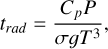
The 0D calculations provide crucial insights into the main chemical mechanisms resulting from atmospheric cooling. In a 1D atmosphere, however, the atmospheric temperature and composition are strongly correlated. The abundances of atmospheric species are affected by the atmospheric temperature changing throughout the column atmosphere. The composition and more specifically the greenhouse properties of the atmospheric mixture also controls the temperature profile. This complexity compels us to combine different calculations using a climate-chemistry model. For that purpose, we coupled the radiative-convective model HELIOS (Malik et al. 2017, 2019a) with the chemistry model VULCAN to perform self-consistent calculations including both radiative transfer and chemical kinetics (photochemistry and thermochemistry). The geochemical calculations of Tian & Heng (2024) are used to set the initial atmospheric composition. It can also be used as a lower boundary condition in VULCAN using a parameterized volcanic flux. As stated previously, we refrain from using this continuous outgassing feature in this work given the lack of constraints regarding the flux. Given the broad range of temperature encountered in our case study, competition between mixing, radiative and chemical timescales is expected which motivates the need to use a self-consistent model. In our atmospheric model, the temperature profile is changed by HELIOS during the VULCAN simulation using the radiative timescale as an iteration time step. The radiative timescale is updated throughout the simulation to modify the time step if needed, it is expressed as follows (Malik et al. 2017):
 (1)
(1)
where P is the pressure, Cp is the heat capacity, σ is the Stefan-Boltzmann constant, g is the gravity and T the atmospheric temperature.
The mean heat capacity of the atmosphere is derived using the abundances of the main atmospheric molecules (CO, CO2, CH4, H2 and H2O) and their Cp at the given surface temperature. Cp(T) of each species is calculated using the thermodynamic data (polynomial constants) from Holland & Powell (1998) also used in the geochemical outgassing calculations (Tian & Heng 2024). The change in temperature is read by VULCAN to update the kinetic constants and reaction rates. Temperature-dependent photo-absorption cross sections and molecular diffusion rates are also changed according to the new temperature conditions.
We include a transit spectra simulator to read the outputs of the atmospheric model. We use the forward model of HELIOS-T first described in Fisher & Heng (2018) which we modified to apply generally for any atmospheric composition and consider temperatures and mixing ratios varying with pressure. HELIOS provides the secondary eclipse emission spectrum of the planet along with the contribution function of different spectral bins to assess the pressure range probed during spectroscopic observations.
Pressure is expected as a critical parameter influencing the dominant chemical regime shaping the atmospheric composition between thermochemistry and photochemistry. Since pressure itself affects both the chemistry and the radiative balance, it is essential to consider both atmospheric chemistry and radiative transfer in the model. The structure of the model is illustrated in Fig. 1. We explore the parameter space of the atmospheric model guided by a specific question, namely, how relative molecular abundances can help constrain the interior fo2 from observations. We want to clarify the role of photochemistry and thermochemistry. If deterministic mechanisms are at play, our aim is to identify how we can correct for them in future applications with a retrieval framework.
Parameters used in the 1D atmospheric simulations of GJ 1132b to assess the influence of atmospheric cooling, photochemistry and mixing on the tracers of fo2.
We focus on a case study of GJ 1132b as recent observations suggest the presence of an atmosphere (Swain et al. 2021; May et al. 2023). In addition, the equilibrium temperature of this exoplanet is close to that of several other super-Earths which ensures that the results and underlying mechanisms identified can be generalized to other objects. We focus on three different end-members of oxygen fugacity and atmospheric surface pressure to evaluate the influence of both parameters. The different end-member cases are summarized in Table 2.
In the outgassing calculation, melt temperature is kept fixed at 1600 K following Gaillard & Scaillet (2014). The process of atmospheric cooling is mainly sensitive to the difference between melt temperature and atmospheric temperature, hence our choice to only vary atmospheric temperature. Activity of graphite is set to ensure an atmosphere rich in carbon (see Table 2). If we consider degassing from a carbon-poor melt, only H2 and H2O would present high abundances that could be detected limiting our ability to infer a quantitative redox state. In the atmospheric model, photochemical haze formation is not included, the surface albedo does not impact our simulations as surface emissivity is set accordingly (albedo = 1 – emissivity). Stellar temperature, radius and mass are set for GJ 1132 (Berta-Thompson et al. 2015) and used to produce the blackbody spectrum in HELIOS. The planet’s surface gravity is also taken from Berta-Thompson et al. (2015). Surface pressure is set according to our three different scenarios (Table 2). The upper boundary pressure (top of atmosphere) is set to 10−7 bar to ensure the accuracy of the UV optical depth and vertical distribution of actinic flux in the 1D atmosphere for the photochemical calculations. The stellar flux of GJ 1132 is subjected to negative values. We thus used the stellar flux of GJ 1214, which presents a similar temperature and radius, with data available as part of the MUSCLES survey (France et al. 2016). The climate model and transit spectra generator includes the opacities of CO (Rothman et al. 2010; Li et al. 2015), CO2 (Rothman et al. 2010), CH4 (Rothman et al. 2010; Hargreaves et al. 2020), H2O (Polyansky et al. 2018) along with collision-induced absorption (CIA) by H2-H2 (Abel et al. 2011). Other CIAs are not included given the lack of data in a broad spectral and temperature range (Chubb et al. 2024). Rayleigh scattering is considered in the atmospheric model (VULCAN, HELIOS, HELIOS-T) for the different species following the formulation in MacDonald & Lewis (2022) using the King factor, refractive index and reference number density with most data taken from Sneep & Ubachs (2005). The water refractive index is pressure-temperature dependent, the data is taken from Murphy (1977) and Schiebener et al. (1990). Vertical mixing described by the eddy diffusion coefficient Kzz is one of the main sources of uncertainty in the chemical model, especially since the temperature is not known a priori. The role of Kzz is assessed and discussed in Sects. 4.1 and 4.2. Molecular diffusion is considered in VULCAN (Tsai et al. 2021) with diffusion coefficients taken from Marrero & Mason (1972) following the formalism in Hu et al. (2012). Photo-absorption and -dissociation cross sections were compiled from the Leiden Observatory database2 in the original study of Tsai et al. (2021). Temperature-dependent cross sections are available for CO2 (150–800 K; Venot et al. 2018) and water (ExoMol3; 300–573 K), although not in the entire range of temperature covered with our simulations (≈400–1600 K). More temperature-dependent cross-section data will be needed in the future to address their influence properly (Chubb et al. 2024). The database of chemical reactions is similar to the one used for the 0D simulations (Sect. 2.2) with the addition of 40 photolysis reactions to consider photochemistry.
 |
Fig. 1 Description of the 1D atmospheric model. Each module of the model is shown with its role and the parameters needed for the simulations. Using iterations between VULCAN and HELIOS following the radiative timescale, the model performs self-consistent calculations of atmospheric chemistry and radiative transfer. The different model parameters mentioned are melt temperature Tm, melt oxygen fugacity fo2, activity of graphite Ac, degassing pressure assumed similar to surface pressure Ps, vertical profile of temperature Tatm and pressure Patm in the atmosphere, eddy mixing coefficient Kzz and vertical profile of volume mixing ratio Xi for each species i. |
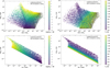 |
Fig. 2 Relative molecular abundances for the different 0D simulations considering a geochemical outgassed mixture cooling to a different atmospheric surface temperature. The black dots show the prediction by outgassing alone. The colored crosses show the predictions with atmospheric cooling. The parameter space covered by these simulations is detailed in Table 1. |
3 Influence of atmospheric cooling on CO2/CO and CH4 production
3.1 Relative molecular abundances: Inferring fo2 and temperature using CO, CO2, and CH4
The relative molecular abundances obtained with the 0D atmospheric cooling simulations are shown in Fig. 2. We remind the reader that these simulations assume thermochemical equilibrium at the planet’s surface temperature set by Ts, lower than the melt temperature. Even after atmospheric cooling, CO2/CO and fo2 remain strongly correlated with a Pearson coefficient at 0.88. The lower correlation compared to the outgassing prediction is explained by a decrease of CO2/CO as Ts increases for a given fo2 (top right panel, Fig. 2). The correlation between CO2/CO and fo2 decreases as the atmospheric temperature departs from the melt temperature, it is thus caused by atmospheric cooling. For Ts between 500 and 1600 K, CO2/CO increases by up to 3–4 orders of magnitude for a given fo2. A constraint on the temperature is therefore essential to correct biases induced by atmospheric cooling.
Figure 2 shows that a single CO2/CO can correspond to a broad range of atmospheric temperature. In other words, this molecular pair cannot be used in observations to infer atmospheric temperature. CO–CH4 conversion is, however, very sensitive to atmospheric temperature (top right panel, Fig. 2). The methane abundance can thus be used to constrain the atmospheric temperature and improve the retrieved fo2. Using the abundances of CO, CO2 and CH4, one can in theory retrieve accurately the oxygen fugacity and atmospheric temperature (top panels, Fig. 2). The feasibility of this latter statement lies in the absolute abundances of each species and their detectability in the spectral range of JWST. In practice, high abundances of methane are found only under reducing conditions. Inferring temperature would be more difficult for oxidized atmospheres. In theory, H2/H2O provides a similar information on fo2 as CO2/CO (bottom left panel, Fig. 2). Although the H2 abundance cannot be retrieved from observations, it suggests that low oxygen fugacity objects would create thicker atmospheres which would affect transit observations through the scale height as discussed in Ortenzi et al. (2020).
3.2 Chemical network and timescales
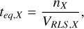
In the geochemical outgassing model, no information on the kinetics is provided as equilibrium between the gas and the melt is assumed (Tian & Heng 2024; French 1966). By calculating the Gibbs free energy and equilibrium constant of each independent reaction (R1)–(R4), one can derive the partial pressures of the main stable species involved in the network (French 1966; Tian & Heng 2024). For the atmospheric calculations, one could use a similar approach where the activity of graphite and oxygen fugacity are replaced by the elemental abundances of the gas mixture (Heng & Tsai 2016; Heng et al. 2016). With chemical kinetics, one understands that the partial pressures of the stable molecules and the timescales of chemical equilibrium are controlled by reactions with the radical products of thermal dissociation, for example, H2O ⟶ OH + H. The abundances of these radicals is changed with temperature. Since we previously showed that atmospheric cooling can strongly modify CO2/CO, we can look at the radicals and reactions to understand why. Figure 3 shows the number density ratios OH/H and CO2/CO as a function of oxygen fugacity and temperature for the different Monte Carlo simulations performed, covering the parameter space described in Table 1. The results teach us that OH/H is correlated to both fo2 and atmospheric temperature. For a given temperature, the fo2 corresponds to a specific O/H or OH/H. We now need to look at the chemical network to understand why the change in radical density also affects molecular abundances such as CO2/CO.
For each simulation, we have a specific atmospheric/degassing pressure, atmospheric temperature and elemental abundances predicted by the outgassing calculations. Using kinetic simulations performed with VULCAN, we evaluate the different reaction rates and find the fastest chemical pathway between two molecules (e.g., CO and CH4) using a Dijsktra algorithm (Dijkstra 1959; Tsai et al. 2018). This analysis gives us the main chemical pathway controlling a specific conversion at a given pressure-temperature and for a given set of elemental abundances. Within this fastest pathway, we identify the rate limiting step (RLS) or slowest reaction which bottlenecks the chemical pathway and controls the timescale. In most scenarios, the chemical timescale can approximated as
 (2)
(2)
where n is the number density (molecules cm−3) of species X at chemical equilibrium and VRLS is the slowest reaction rate in the fastest pathway (molecules cm−3 s−1).
The outgassing model predicts a broad range of elemental abundances, although C/O is usually below 1 given the difficulty in producing CH4-rich atmospheres. O/H varies significantly depending on fo2 giving very high metallicities poorly studied as previous work focused on hot Jupiters or hot Neptunes and the effect of C/O (Moses et al. 2011, 2013a,b; Venot et al. 2015; Tsai et al. 2018). Our network analysis shows that CO–CO2 and H2− H2O conversions are always controlled by the following scheme in the entire parameter space (pressure, temperature, elemental abundances):
 (R5)
(R5)
 (R6)
(R6)
net: CO+H2O ⟷ CO2 + H2
From this pathway, one can understand why variations of CO2/CO and OH/H are directly correlated. First, the increase in CO2/CO with fo2 at a given temperature is caused by the increase in OH/H favoring the oxidation of CO. An increase in fo2 corresponds to an increase in O/H and therefore OH/H. However, OH/H also varies with temperature for a given O/H, as thermal dissociation rates of water and molecular hydrogen vary differently with temperature (Fig. 3). H2/H2O is controlled by OH/H and therefore decreases with increasing fo2 and increasing temperature. This analysis explains the trends of relative abundances as a function of fo2 and temperature in Fig. 2 (bottom panels). CO2/CO on the other hand increases with increasing fo2 but decreases with increasing temperature. This result can seem counter-intuitive but is explained by the balance in elemental abundances. The decrease in OH/H and H2O/H2 with increasing temperature at a given fo2 leads to an increase of CO2/CO to conserve elemental abundances and especially O/H. The trends of relative molecular abundances for CO2, CO, H2 and H2O are completely explained following the change of the radical density ratio OH/H with temperature and fo2.
We also evaluated CO–CH4 conversion for the different simulations. We identified the following scheme:
 (R7)
(R7)
 (R8)
(R8)
 (R9a)
(R9a)
 (R9b)
(R9b)
 (R10a)
 (R10b)
 (R11a)
 (R11b)
 (R12)
(R12)
 (R13a)
 (R13b)
 (R14)
(R14)
 (R15)
(R15)
net: CO + 3 H2 ⟷ CH4 + H2O
This general scheme is valid for the different simulations performed, although some steps can be associated with different reactions depending on the temperature, pressure and elemental abundances. The oxygenated species produced during CO–CH4 conversion are, however, similar. As our outgassing calculations predict C/O≤1, the CO–CH4 scheme involves primarily oxygenated species such as methanol and formaldehyde. For C/O≥1, the fastest pathway would also involve saturated and unsaturated reduced hydrocarbons (Moses et al. 2011, 2013a; Venot et al. 2015; Tsai et al. 2018).
The reaction converting CH3O−CH3 OH involves either H2 and H (R10a) or H2O and OH (R10b) depending on the oxygen content in the atmosphere and more specifically depending on O/H. The reaction (R10a) dominates for O/H < 0.5, whereas (R10b) dominates for higher O/H. A similar result is found for the CH3-CH4 conversion. For high O/H, oxidation of methane dominates through reaction (R13b), whereas hydrogenation dominates for lower O/H (R13a). The CH3-CH4 reaction might be changed with H2S when sulfur is included (Liggins et al. 2023), although this depends on the sulfur content in the mixture.
The reaction converting CH3-CH3OH or CH3-CH2OH depends on the temperature-pressure conditions. Using the analysis of the reaction rates in the VULCAN simulations, we find that (R11a) and (R12) are competing at temperatures above ≈900 K. Reaction (R11a) dominates at high pressure as methanol formation/dissociation is pressure-dependent. Reaction (R11a) is indeed a three-body reaction which becomes inefficient at low pressures. The two-body reaction (R12) becomes more efficient than (R11a) at low pressures. The fastest pathway is thus going directly from CH2OH to CH3 without methanol at low pressure. The pressure value marking the transition from (R11a) to (R12) depends on the temperature. This pressure value increases with temperature from about 10−2 bar at 900 K to 10 bar at 1600 K in agreement with the analysis of Tsai et al. (2018). At temperatures below 900 K, (R11a) and (R11b) are competing. For a high OH/H, (R11a) would dominate as it involves OH compared to (R11b) involving H. The transition between (R11a) and (R11b) for the limiting reaction depends on both temperature and O/H since both parameters affect OH/H.
For every simulation, either (R11a), (R11b) or (R12) is identified as the limiting reaction (RLS) for the thermochemical production of methane. The CO–CH4 conversion requires the dissociation of three bonds binding C and O together. The timescale of this conversion is limited by the dissociation of the last bond in methanol or CH2OH. These results are in agreement with previous analyses of CO–CH4 conversion for exoplanet atmospheres (Moses et al. 2011; Tsai et al. 2018; Liggins et al. 2023). We refer the reader to previous work by Tsai et al. (2018) for a more detailed analysis of RLS changes in various conditions of pressure, temperature and elemental abundances.
Our results show that the change in OH/H controlled by oxygen fugacity and temperature has a significant impact on the CO–CH4 and CO–CO2 conversions. Differences are thus expected in terms of timescales. Figure 4 presents the thermochemical timescales of CO derived for each simulation as a function of temperature, pressure and fo2. In general, a broad range of thermochemical timescale is possible for a single temperature depending on the fo2 and pressure (Fig. 4).
It was previously shown that the timescale of CO can be derived by identifying the RLS of the CO–CH4 conversion for low metallicity atmospheres representative of hot Jupiters (Tsai et al. 2018). For high O/H, that statement is no longer valid, as the oxidation of CO with the radical OH becomes more efficient than its hydrogenation that initiates the CO–CH4 conversion. The timescale of CO can be approximated using (R5) as RLS in Eq. (2) when the rate of (R5) is higher than the rate of (R7). We note that the timescale of CO at low temperatures and high fo2 joins the timescales trend obtained for low fo2 (Fig. 4, bottom panel) and is thus controlled by CO–CH4 conversion. This stems from the decrease in OH/H at a lower temperature and the resulting less efficient CO oxidation relative to hydrogenation. For low O/H, the timescale of CO is controlled by CO–CH4 conversion and thus by the RLS in the given pressure-temperature conditions.
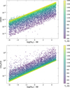 |
Fig. 3 Number density ratio OH/H (top) and CO2/CO (bottom) at chemical equilibrium as a function of oxygen fugacity and atmospheric (surface) temperature. The parameter space explored in the different simulations is summarized in Table 1. |
4 Case study using a climate-chemistry model: How pressure, temperature, mixing, and UV photons impact the atmospheric tracers of fo2
The trends in relative molecular abundances and timescales observed inFigs. 2–4 with atmospheric cooling (thermochemistry alone) are caused by the changes in OH/H with both temperature and fo2. It is thus important to constrain atmospheric temperature from observations to improve the retrieval of fo2. Generally speaking, the thermochemical timescales are shorter at increasing temperatures, pressures and fo2. Below 700−800 K, the timescale can be very long depending on O/H and pressure (Fig. 4). At these temperatures, equilibrium chemistry might not dominate over photochemistry and both must be considered carefully. The generalization of the timescales for photochemistry is difficult as it depends on several parameters including atmospheric composition, temperature, pressure, orbital distance and the distribution of stellar flux across the 1D column atmosphere. In this section we perform 1D modeling including climate and chemical calculations (see Table 2) to understand the combined role of photochemistry and thermochemistry, and their influence on the molecular abundances of C–H–O species.
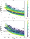 |
Fig. 4 Thermochemical timescales of CO as a function of temperature, pressure, and fo2 for the different simulations. Two branches are observed, as the timescale is controlled by CO–CO2 conversion at high fo2 (high O/H) and by CO–CH4 conversion at low fo2 (low O/H). The parameter space explored in these 0D simulations is detailed in Table 1. |
4.1 Production of methane in volcanic atmospheres: A chemistry-climate feedback
Previous outgassing calculations showed that methane-rich degassing only occurs at low melt temperature and high degassing pressure (Wogan et al. 2020; Tian & Heng 2024). However, methane can be produced by atmospheric cooling (thermochemistry) using the degassed CO and H2 (Liggins et al. 2023). CH4 is a strong greenhouse gas that can significantly affect the temperature profile. For our simulation with a surface pressure of 0.01 bar, we found CH4 buildup by atmospheric cooling to be inefficient given the low surface temperature around 650 K. CH4 is produced efficiently in the 1 and 100 bar simulations however. Figure 5 shows the evolution of temperature and CO–CH4 mixing ratios during the process of atmospheric cooling for the two end-member fo2 (IW-3 and IW+3) with a surface pressure of 1 bar. We focus on this 1-bar surface pressure simulation to describe the mechanism forming methane. In the low fo2 scenario (IW-3), the initial atmosphere presents a surface temperature much cooler than the high fo2 scenario. An oxidized atmosphere made of CO2−H2O indeed possesses a higher IR opacity compared to the reduced CO–H2 atmosphere. The 900 K initial surface temperature of the low fo2 scenario is explained by the high abundance of water in the atmosphere with a smaller contribution of H2−H2 CIA. The surface temperature of the low fo2 atmosphere, however, increases by 300 K in only a few years, whereas the high f2 surface temperature is stable over time (top panels, Fig. 5). Both simulations converge to a similar final surface temperature, although warming is driven by CO2 and H2O in the high fo2 case, and by H2O and CH4 in the low fo2 case.
Figure 5 (left panels) shows that the increase in surface temperature in the low fo2 scenario is correlated with the increase in CH4 and decrease in CO mixing ratios. CO–CH4 conversion indeed favors methane at a temperature of 900 K, and the chemical timescale is still short (Fig. 4), thus allowing fast methane buildup. At 900 K, chemical equilibrium would, however, predict a methane mixing ratio above the CO mixing ratio (see dashed black curve, Fig. 5, middle left panel), whereas our simulation shows that the methane abundance stabilizes around 5.10−3. This is explained by the radiative properties of methane limiting its own buildup as the abundance of CH4 is very sensitive to the temperature. The increase of temperature caused by the increase in methane mixing ratio indeed changes the CO–CH4 conversion making CO more stable at the final temperature of ≈1200 K. In other words, the strong IR opacity of methane prevents its buildup above percentage level. This statement is true as the radiative timescale is here shorter than the chemical timescale leading to a climate feedback evolving progressively with the chemistry. In the high fo2 scenario, the higher O/H favors oxidation of CO (R5) making methane buildup less efficient (right panels, Fig. 5). Liggins et al. (2023) previously showed that high methane abundances can be obtained in low fo2 conditions by atmospheric cooling, although their simulations do not consider this climate feedback which likely lead to biases in the final abundances. In both fo2 scenarios, equilibrium chemistry would predict high methane abundances in the upper atmosphere, at pressures below 0.1 bar, given the lower atmospheric temperature (middle panels, black dashed curves, Fig. 5). Vertical mixing, however, quenches the methane abundance at higher pressures making the observed abundances dominated by disequilibrium chemistry. In the case of an oxidized rocky interior, for instance, the abundances of CO and CH4 in the lower atmosphere are at chemical equilibrium (Fig. 5, middle & bottom right panels), whereas their abundances in the upper atmosphere are homogenized, a process referred to as mixing-driven quenching. This occurs as mixing become more efficient (shorter timescale) than chemical equilibrium in the upper atmosphere following the decrease in temperature and pressure (Moses 2014; Tsai et al. 2017). The quench point refers to the altitude (or pressure) at which the timescale of mixing becomes equal to that of chemical equilibrium. In other words, one must know the pressure-temperature conditions in the lower atmosphere close to the surface to interpret the methane abundance quenched by mixing in the upper atmosphere.
In the high surface pressure scenario (100 bar) of the low fo2 end-member simulation, methane is more stable and can build up to higher abundances reaching percentage levels (not shown). In general, the methane buildup and lower ratio CO/CH4 suggest the presence of a thick atmosphere leading to high temperatures at the surface. High-pressure/High-temperature chemistry dominates the observables as thermochemistry and mixing-driven quenching is faster than photochemistry in these conditions. Kzz does not affect the final outcome of the feedback in terms of temperature and mixing ratio. It however affects the evolution over time as the mixing and radiative timescales are competing. For low Kzz values, the CH4 buildup starting in the lower atmosphere at higher pressures is not transported upwards fast which affects the radiative feedback. In the 100 bar scenario, the chemical timescale is shorter than the radiative timescale making the model converge fast, with fewer iterations. The dominant chemical mechanism changes for lower pressures where photochemistry dominates the evolution, this is discussed in Sect. 4.2.
If one would change the planet’s orbital distance, the resulting effect on the surface temperature would also modify the outcome of the climate-chemistry feedback induced by methane. This process is therefore sensitive to the atmospheric redox state and surface temperature. This latter parameter is itself controlled by the abundances of greenhouse gases, the surface pressure and the orbital distance.
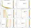 |
Fig. 5 Temporal evolution of temperature and CO–CH4 volume mixing ratios in a 1-bar atmosphere around GJ 1132b considering two end-member oxygen fugacities (IW-3 and IW+3). We assumed Kzz = 107 cm2/s. The initial atmospheric composition was set by the outgassing model and is shown with the blue curve corresponding to t=0 s. We consider fo2 = IW-3 and Ac = 10−2 for the low oxygen fugacity end-member (left panels) and fo2 = IW+3 and Ac = 10−6 for the high oxygen fugacity end-member (right panels). The dashed black curve shows the prediction of chemical equilibrium without vertical mixing computed with FastChem using the initial state of the atmosphere (abundances set by outgassing). |
4.2 Atmospheric CO2/CO as a tracer of the interior fo2: Effect of thermochemistry and photochemistry
As discussed in Sect. 3, CO2/CO decreases with increasing temperature driven by the change in OH/H. In a 1D column atmosphere, the CO–CO2 abundances will change throughout the atmosphere given the decrease of temperature with altitude. The vertical abundances of the main species involved in the net reaction CO + H2O ⟷ CO2 + H2 are shown in Fig. 6 for the two end-member fo2 (IW-3 and IW+3) simulations considering a 1-bar atmosphere. Since CO and CO2 quench at a lower pressure than CH4, the change of temperature in the lower atmosphere is important and will control their abundance in the upper atmosphere (i.e., in the region probed during spectroscopic observations). For both fo2 scenarios, we observed that CO2/CO increases with altitude caused by the decrease in temperature (Fig. 6). Kzz controls the quench point and thus the CO2/CO in the upper atmosphere.
In our simulations, the CO2/CO predicted by outgassing can change in the atmosphere by a factor of ≈ 2−3 depending on the temperature and mixing rate (see Fig. 6). In theory, CO2/CO could change by several orders of magnitude (Fig. 2) as discussed in Sect. 3 but the long chemical timescales obtained for the low temperature simulations make thermochemistry inefficient compared to photochemistry. This change of CO2/CO by a factor of 2−3 is reasonable and suggest that the molecular abundances in the atmosphere still encode crucial information on the redox state of the interior.
Although thermochemistry dominates the vertical abundances of the species in the 1-bar and 100-bar simulations given the high surface pressure and temperature, photochemistry dominates the evolution in the 0.01-bar simulation. The temporal evolution of the temperature profile and vertical mixing ratios of CO2, CO and H2O are shown in Fig. 7 for a 0.01-bar atmosphere produced around GJ 1132b from a reduced rocky interior (IW-3). Analysis of the chemical network reveals an evolution similar to thermochemistry with CO + H2O ⟷ CO2 + H2 as a net reaction:
 (R16)
(R16)
 (R17)
(R17)
 (R18)
(R18)
net: CO + H2O ⟶ CO2 + H2
The change here is that radicals OH and H are produced by photo-dissociation in the upper atmosphere instead of thermo-dissociation in the lower atmosphere. In the low fo2 scenario (IW-3), the abundance of CO exceeds that of water. The high abundance of water, however, leads to an efficient production of the OH radical which oxidizes and destroys CO. Over long periods of time (tens to hundreds of thousands of years), the loss of water and CO becomes significant with the oxidation of CO leading to an increase of CO2 abundances. The photolysis of CO2 reproduces CO but this process is less efficient than the water photolysis and oxidation of CO. As the system evolves over time, water mixing ratio decreases and CO will stabilize to an abundance resulting from a balance between destruction by oxidation and production by CO2 photolysis. Overall, CO2/CO increases by ≈1 order of magnitude in tens of thousands of years (Fig. 7). The temperature profile changes over time but only in the upper atmosphere (Fig. 7, top left panel) since the initial stratospheric inversion induced by water (Malik et al. 2019b) is removed as a result of its photochemical loss. This photochemical mechanism suggests that photochemistry can introduce a bias in CO2/CO, although the long timescale of this process would make it inefficient if the planet is still volcanically active.
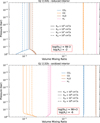 |
Fig. 6 Vertical volume mixing ratios of CO, CO2, H2, and H2O for the 1-bar atmosphere scenario of GJ 1132b with two end-member oxygen fugacities (IW-3 and IW+3). The initial atmospheric composition is set by the outgassing calculation. We consider fo2 = IW-3 and Ac = 10−2 for the low oxygen fugacity end-member (top panel) and fo2 = IW+3 and Ac = 10−6 for the high oxygen fugacity end-member (bottom panel). Different mixing efficiencies are shown (eddy coefficient Kzz) affecting the molecular abundances at the quench point (e.g., CO2/CO). The pressure-temperature profiles of both scenarios are shown in Fig. 5 (top panels). |
4.3 Overall influence of pressure and fo2 on atmospheric abundances
The chemical regime controlling CO2/CO, i.e. photochemistry or thermochemistry, is mainly influenced by oxygen fugacity itself (through varying O/H), orbital distance and surface pressure. All of these parameters influence the surface temperature and thus the kinetic competition between photochemistry and thermochemistry. Since the stellar flux and orbital distance are well constrained for the different rocky exoplanets observed, the main parameters one should assess carefully to interpret relative molecular abundances are surface pressure and fo2. Mixing can be important, although it should affect the quenched relative abundances by a factor of 2−3 at the most (Fig. 6). If the atmosphere is thin (low surface pressure and temperature) and continuously replenished by geochemical outgassing, the CO2/CO will be preserved given the long timescales of the photochemical mechanism (see Sect. 4.2).
For each scenario, we calculated with HELIOS the contribution function at different spectral bins to assess the pressure and temperature probed in emission. The contribution function quantifies the weight of each atmospheric layer in the emission of radiation escaping at the top of the atmosphere. In spectral bins with high molecular opacity, the radiation escaping at the top of the atmosphere mainly originates from the low-pressure layers of the upper atmosphere. In a spectral range with no clear molecular opacity, deeper layers are probed. The contribution function at different spectral bins corresponding to transparent windows and absorption peaks of CO2 and CH4 mainly is shown in Fig. 8 (top right panel) for the high fo2 (IW+3) 1-bar scenario. We clearly observe that the deep atmosphere is probed at 3.9 μm, between the absorption peaks of CO2 and H2O.
Figure 8 (top left panel) shows the emission spectra (expressed as ratio of flux emitted by planet relative to that emitted by the star) for the two different fo2 end-member scenarios assuming a 1-bar atmosphere. For the high fo2 scenario (IW+3), emission between 3.2 and 4.2 μm is high as we are probing the deeper atmospheric layers in agreement with the information provided by the contribution function (Fig. 8, top right panel). For the low fo2 scenario, we see a significant difference in this spectral range as methane is absorbing around 3.4 μm. In other words, the difference between the two fo2 end-members in emission is mainly reflected between 3.2 and 4.2 μm where the presence or absence of methane leads to a change in the temperature/pressure probed. In the case where methane is not present, i.e. high fo2, the temperature of the deep atmosphere could be inferred from these spectroscopic observations. We remind the reader that the absence of methane can also be explained by a thin atmosphere with low surface temperature in a low fo2 scenario.
In the region between 10 and 15 μm previously used to assess the presence of a thick CO2 atmosphere around Trappist-1c (Zieba et al. 2023) and −1b (Ducrot et al. 2024), we observe a change between the low fo2 and high fo2 scenarios. In both cases, the 15-μm CO2 band is observed but the ratio of signal between 12 and 15 μm is different and traces the abundances of water. This ratio will likely depend strongly on H2O/CO2 and therefore does not directly reflect fo2.
Figure 8 (bottom panels) shows the simulated transmission spectra of GJ 1132b for a 1-bar atmosphere and two different fo2 (IW-3 and IW+3). In transmission, variations between low fo2 and high fo2 scenarios mainly lie in the abundance of methane and carbon monoxide as shown in Fig. 8 (bottom panels). In the low fo2 case, the CO–H2 atmosphere is seen with the clear signatures of methane at 2.3 and 3.4 μm and CO dominating the contribution at 4.7 μm. CO2 is still abundant and detected in the low fo2 case using its 4.4 μm feature. In the high fo2 scenario (bottom right panel, Fig. 8), the high abundances of CO2 and H2O dominate the spectrum and contribute significantly at 4.7 μm given the lower opacity and abundance of CO. Retrieving accurately high CO2/CO might be challenging as the data would probably be fitted efficiently without considering the contribution from CO. Future work should assess in detail the limitations in inferring CO2/CO for rocky exoplanet atmospheres using a retrieval framework. Only with this detailed retrieval analysis, one could evaluate how accurate the CO2/CO value can be.
In our analysis, we observed that the probed pressure at the peak of the opacity bands of CO2, CO, CH4, and H2O is below 0.1 bar (top right panel, Fig. 8). The probed mixing ratio thus corresponds to the quenched value controlled by vertical mixing. Our analysis suggest that the effect of Kzz has negligible impact on the transit spectra as the variation in mixing ratios are small for the dominant atmospheric species and usually within 50% for the secondary species (CO–H2 in high fo2 case and H2O−CO2 in low fo2 case). In Fig. 9, we review the quenched abundances of the different simulations across the Ps−fo2 space and summarize the changes in CO2/CO, caused by atmospheric cooling for a 1-bar and 100-bar atmosphere and photochemistry for a 0.01-bar atmosphere, compared to the outgassing prediction. We also assess the changes in CO2/CH4 as the distinct signatures of methane in transit spectra are easier to resolve in comparison to CO (Fig. 8, bottom panels).
In all the scenarios, CO2/CO is increased (Fig. 9, top panel) by atmospheric chemistry compared to the outgassing prediction following the chemical mechanisms described in Sects. 3.2 and 4.2. With thermochemistry, the change in CO2/CO remains below one order of magnitude as the high abundances of greenhouse gases in volcanic atmospheres (CH4, CO2 and H2O) tend to produce high surface temperatures with a relatively low difference with the melt temperature. Photochemistry can modify CO2/CO for thin atmospheres, although this process occurs over timescales likely longer than the replenishment by outgassing. These two mechanisms changing CO2/CO in the atmosphere are summarized in Fig. 9 (bottom panel). Following the outgassing calculations, CO2/CO changes by one order of magnitude when fo2 varies by two orders of magnitude (see Fig. 9, top panel). The effect of atmospheric chemistry introduces a limit into how accurate one can be in inferring fo2 if the temperature of the quench point cannot be constrained. We estimate this bias around 1–2 orders of magnitude.
Figure 9 (top panel) shows that CO2/CH4 decreases following the thermochemical buildup of methane induced by atmospheric cooling for thick atmospheres (1-bar and 100-bar cases) and described in Sect. 4.1. At fo2 around IW and below, CO2 and CH4 coexist at high abundances. CO2/CH4 can help constrain atmospheric fo2 if the CO abundance cannot be retrieved accurately. We emphasize that unlike CO2/CO and fo2, the correlation between CO2/CH4 and fo2 is not linear (see Fig. 9, top panel) as it also depends on the hydrogen budget; however, it provides a crucial insight into the redox state. Above IW, CO2/CH4 is very high, and methane will likely not be observed given its low stability in an atmosphere with high O/H (see Fig. 8, bottom right panel). The high abundance of water and CO2 and the absence of methane might be the best indicator of high fo2 scenarios, although constraining the exact fo2 value is limited by the detection efficiency of CO. At low fo2, the co-existence of CO, CH4, and CO2 could be constrained and provide crucial information on the interior fo2 and the atmospheric temperature. CO/CH4 can help constrain the atmospheric temperature (Fig. 2, top-right panel), whereas CO2/CO or CO2/CH4 can be used to constrain fo2 (Fig. 9, top panel). Figure 9 also shows that the difference in CO2/CO and CO2/CH4 between the 1-bar and 100-bar scenarios is small, below the accuracy expected with JWST. This tells us that these relative molecular abundances are not clearly correlated to the surface pressure. Surface pressure is, however, one of the main parameters affecting the outcome of atmospheric chemistry as it also controls temperature. A change in pressure from 1 bar to 100 bars does not significantly change the methane abundances. Methane is more stable at high pressure, but it is also less stable at a high temperature. Although a thick atmosphere has the ideal pressure conditions for methane to be stable, it also creates warmer conditions that will tend to de-stabilize methane. In the end, the methane abundance is not changed significantly compared to a 1-bar atmosphere. Since retrieving Ps from observations is difficult (e.g., Heng & Kitzmann 2017), retrieval framework and fo2 inference should consider this parameter carefully.
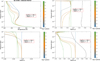 |
Fig. 7 Temporal evolution of temperature and volume mixing ratios of CO2, H2O, and CO in the 0.01-bar atmosphere scenario of GJ 1132b (with Kzz = 105 cm2/s) produced from a reduced rocky interior (IW-3). The dashed back curve shows the prediction by equilibrium chemistry without mixing and computed with FastChem using the initial abundances predicted by outgassing. |
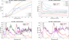 |
Fig. 8 Predictions of observation for a 1-bar atmosphere produced from a low fo2 and high fo2 rocky interior for GJ 1132b. (Top left panel) Emission spectra of the high fo2 and low fo2 1-bar atmosphere. Blackbody emission spectra at different temperatures are plotted for comparison (dashed curves). (Top right panel) Contribution function calculated with HELIOS to assess the pressure and temperature probed in emission with different spectral bins for the high fo2 case. (Bottom panels) Transit spectra focusing on the NIRSpec range of JWST, with the contribution of the different species on the observed signatures for the low fo2 scenario (left) and high fo2 scenario (right). |
5 Model limitations and discussions
5.1 Limitations of the model
The geochemical outgassing calculations following the approach of French (1966) provide a simple solution for the partial pressure of volatiles in the C−H−O fluid system, although it does not consider their solubility in a silicate melt. In practice, one needs to extend the simple system in French (1966) to include gas-melt equilibria, for example for water (dissolved as OH−) and CO2 (dissolved as carbonate  ), following the formalism in Iacono-Marziano et al. (2012), Gaillard & Scaillet (2014), Burgisser et al. (2015) or Liggins et al. (2020). Ascension of magma and surface degassing is typically simulated by solving the set of gas-gas and gas-melt equilibria equations at decreasing pressure until soluble species ex-solve from the melt and the surface pressure is reached. This approach is used in the D-compress and EVolve models of Burgisser et al. (2015) and Liggins et al. (2022) respectively, both used for applications in planetary and exo-planetary sciences.
The added complexity in these calculations leads to additional model parameters including mantle melt fraction, partition coefficients of the species and volatile budget, all of which are largely unconstrained for exoplanets. Our approach focuses on the main parameter affecting gas speciation, oxygen fugacity, using simple calculations that can be easily included in the analysis of JWST data to assess the error on the retrieved fo2. The solubility of water could, however, affect the O/H budget of the atmosphere and change the outcome of thermochemistry and photochemistry. Water is indeed favored at higher pressures in the gas phase (Tian & Heng 2024), although water solubility becomes important above 1 bar (Gaillard & Scaillet 2014; Bower et al. 2022). Since the change of CO2/CO caused by atmospheric cooling and photochemistry is directly correlated to O/H and the abundance of water, solubility must be considered carefully when applying this approach to warm rocky exoplanets. For instance, the increase in CO2/CO for thin atmospheres shown in Fig. 9 (top panel) and driven by photochemistry would change in an atmosphere depleted in water vapor. In a similar way, atmospheric escape can change the O/H atmospheric budget over time. Given the conclusions of this study, both melt solubility and atmospheric escape should be considered in future work to assess in greater details their influence on the variations of O/H compared to fo2. This complexity increases the difficulty in inferring the interior fo2 from observations especially since the surface pressure (controlling solubility) and the escape history are not constrained from observations.
Given the high solubility of N in the melt at low fo2 (Bernadou et al. 2021) and its significant impact on the atmospheric abundances of NH3 (Shorttle et al. 2024), we leave these calculations for a future study where solubility will be included in the calculations. N-rich volcanic atmospheres are expected (Liggins et al. 2022, 2023), one might foresee a similar effect of O/H on the N2-NH3 conversion with N2 favored at high O/H. The effect of NH3 on the radiative-chemical feedback discussed for CH4 (Fig. 5, Sect. 4.1) should be assessed given its high IR opacity and its thermochemical stability also strongly dependent on temperature.
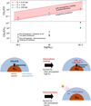 |
Fig. 9 Impact of atmospheric cooling (thermochemical cooling) and photochemistry on the relative molecular abundances, namely, CO2/CO and CO2/CH4, used as atmospheric tracers for the interior fo2. (Top) Relative molecular abundances CO2/CO and CO2/CH4 at the quench point for different end-member cases of Ps and fo2 (see Table 2). The black marker shows the prediction by outgassing alone and the colored markers show the prediction including atmospheric chemistry. (Bottom) Schematic summarizing the main atmospheric processes affecting CO2/CO and methane buildup. The terms “thick” and “thin” atmospheres are used respectively to mark the transition from a regime dominated by thermochemistry toward a regime dominated by photochemistry. This transition is not quantified using pressure ranges as other variables must be considered including orbital distance and O/H (see Sect. 4.2). |
5.2 Implications for JWST observations
For rocky exoplanets, recent observations of 55 Cancri e (Tsiaras et al. 2016; Hu et al. 2024), GJ 486b (Moran et al. 2023) or GJ 1132b (Swain et al. 2021; May et al. 2023) suggest the presence of an atmosphere where the main gas components can be identified. Although the observations of Trappist-1c (Zieba et al. 2023), Trappist-1b (Ducrot et al. 2024) and LHS 475b (Lustig-Yaeger et al. 2023) point to a thin atmosphere or no atmosphere, the data quality suggest that a thick atmosphere should be detected if present. Even in emission, one should expect to resolve CO2 and H2O bands efficiently if enough transits were accumulated (Piette et al. 2022). The current observations are limited by the spectral range and the presence of cool stellar spots leading to detections of methane and water bands that might not originate from the planet’s atmosphere (May et al. 2023; Moran et al. 2023). Despite these limitations, interpretation of molecular detections in rocky exoplanet atmospheres is starting including reasoning around the interior redox state (Heng 2023; May et al. 2023; Hu et al. 2024). The variations in the secondary eclipse observations of 55 Cancri e could be caused by transient degassing unbalanced with atmospheric escape given the very short orbital period of the planet (Heng 2023). Recent observations suggest an atmosphere rich in CO2 and/or CO as revealed by the clear absorption between 4 and 5 μm (Hu et al. 2024). The large error bars on the data, however, do not allow for clear constraints on CO2/CO and fo2 (Hu et al. 2024). Our theoretical simulations do not indeed predict a clear distinction between high fo2 and low fo2 between 4 and 5 μm (Fig. 8, top left panel). Additional measurements of 55 cancri e around the 15-μm CO2 feature with MIRI might help constrain the main atmospheric species and the ratio CO2/CO. For GJ 1132b, the detection of H2O and CH4, if not caused by stellar spots, limits the interpretation of the redox state as CO2 and CO abundances are not well constrained (May et al. 2023). The recent data suggest a H2O-dominated atmosphere which could be explained by a thin atmosphere produced from an oxidized interior. H2O-dominated atmospheres are unlikely at high pressures because of the high solubility in melts (Bower et al. 2022; Sossi et al. 2023) and recent emission observations of GJ 1132b rule out the presence of a thick atmosphere (Xue et al. 2024).
Our work is also relevant for sub-Neptune planets as recent observations suggest that a magma ocean could be present beneath the thick H2 envelope with degassing explaining a high metallicity (Shorttle et al. 2024; Benneke et al. 2024). In addition, the high atmospheric pressure scale height of these objects make them ideal targets with JWST. The high abundances of CH4 and CO2 inferred from JWST observations of K2-18b, although compatible with biotic methane emissions in an ocean planet with a shallow H2 envelope and habitable surface temperature (Madhusudhan et al. 2023), could also be explained by a thick H2 atmosphere with high metallicity around 100 Xsolar (Wogan et al. 2024). The co-existence of CO2-CH4 at high abundances in the atmospheres of K2-18b may be explained by a deep magma ocean with reducing conditions at equilibrium with the thick H2 atmosphere (Shorttle et al. 2024). Following our study, the high abundances of methane in the atmosphere of K2-18b point to a low OH/H, although one would need to constrain the atmospheric temperature to retrieve the fo2 with greater accuracy. At these high metallicities and low oxidation states, abundances of CO higher than CO2 are expected (Shorttle et al. 2024) but not suggested by the retrieval analysis of Madhusudhan et al. (2023). The difference between the habitable shallow atmosphere and warm deep atmosphere scenarios lies in the CO abundance relative to CO2 and CH4. As described in Sect. 4.3, CO could be unconstrained given its low IR opacity and its main band overlapping with that of CO2. CO2/CH4 can, however, be seen as a tracer of fo2 as well (see Sect. 4.3). More quantitatively, Madhusudhan et al. (2023) and Benneke et al. (2024) suggested CO2/CH4 ≈ 1 for both K2−18b and TOI-270d respectively which would roughly correspond to a fo2 around IW-3 (see Fig. 9) if we consider atmospheric cooling. A more complex model considering equations of state is needed for sub-Neptunes to accurately consider the high pressure conditions at the boundary between atmosphere and rocky body. The nature of these sub-Neptune planets is still unclear, although the composition of the atmosphere may be hybrid, made of primitive H2-He mixed with heavier gases from volcanic degassing (Benneke et al. 2024). One would need to assess the CO2/CH4 and if possible CO2/CO for several sub-Neptune planets with different equilibrium temperatures to confirm the deep magma ocean hypothesis and help unveil the nature of these mysterious objects.
6 Conclusions
Using relative abundances of the simple molecules (CO, CO2., CH4, and H2O) that are starting to be constrained from observations of rocky exoplanet atmospheres with JWST, the implications for the redox state of the rocky interior can start to be discussed. The relative molecular abundance CO2/CO provides crucial information given the direct correlation with oxygen fugacity. This relative abundance can, however, be modified in the atmosphere by thermochemical cooling (referred to as atmospheric cooling) and photochemistry. Our numerical simulations revealed the following:
Thermochemical cooling leads to an increase of CO2/CO by up to one order of magnitude, which would bias the inferred fo2 by two orders of magnitude. This process is strongly dependent on the temperature difference between the melt and the quench point in the atmosphere. Constraints on the atmospheric temperature can help correct the bias on the retrieved fo2;
Photochemistry leads to an increase of CO2/CO over long timescales and is driven by the oxidation of CO via the photolysis of water vapor. The bias on CO2/CO would depend on the competition between outgassing flux and photochemistry;
The transition between these two chemical regimes (i.e., photochemistry-driven and thermochemistry-driven) is not associated with a single value of temperature. It depends not only on surface pressure and temperature but also on the redox state of the atmosphere (via O/H). Thick atmospheres (high surface pressure and temperature) with high fo2 tend to be driven by thermochemical cooling, whereas thin atmospheres with low fo2 tend to evolve controlled by photochemistry.
Acknowledgements
T.D. acknowledges support by the “ADI 2021” project funded by the IDEX Paris-Saclay, ANR-11-IDEX-0003-02. T.D. and N.C. thank the European Research Council for funding via the ERC OxyPlanets project (grant agreement No. 101053033).
References
- Abel, M., Frommhold, L., Li, X., & Hunt, K. L. C., 2011, J. Phys. Chem. A, 115, 6805 [NASA ADS] [CrossRef] [Google Scholar]
- Adibekyan, V., Dorn, C., Sousa, S. G., et al. 2021, Science, 374, 330 [NASA ADS] [CrossRef] [Google Scholar]
- Ballhaus, C., Berry, R. F., & Green, D. H., 1991, CoMP, 107, 27 [Google Scholar]
- Batalha, N. M., Rowe, J. F., Bryson, S. T., et al. 2013, ApJS, 204, 24 [Google Scholar]
- Baulch, D. L., Cobos, C. J., Cox, R. A., et al. 1992, J. Phys. Chem. Ref. Data, 21, 411 [NASA ADS] [CrossRef] [Google Scholar]
- Benneke, B., Roy, P.-A., Coulombe, L.-P., et al. 2024, arXiv e-prints [arXiv:2403.03325] [Google Scholar]
- Bernadou, F., Gaillard, F., Füri, E., Marrocchi, Y., & Slodczyk, A., 2021, Chem. Geol., 573, 120192 [Google Scholar]
- Berta-Thompson, Z. K., Irwin, J., Charbonneau, D., et al. 2015, Nature, 527, 204 [Google Scholar]
- Borucki, W. J., Koch, D., Basri, G., et al. 2010, Science, 327, 977 [Google Scholar]
- Borucki, W. J., Koch, D. G., Basri, G., et al. 2011, ApJ, 736, 19 [Google Scholar]
- Bower, D. J., Hakim, K., Sossi, P. A., & Sanan, P., 2022, Planet. Sci. J., 3, 93 [NASA ADS] [CrossRef] [Google Scholar]
- Brewer, J. M., & Fischer, D. A., 2016, ApJ, 831, 20 [CrossRef] [Google Scholar]
- Buchhave, L. A., Latham, D. W., Johansen, A., et al. 2012, Nature, 486, 375 [NASA ADS] [Google Scholar]
- Burgisser, A., Alletti, M., & Scaillet, B., 2015, Comput. Geosci., 79, 1 [Google Scholar]
- Chubb, K. L., Robert, S., Sousa-Silva, C., et al., 2024, RASTI, 3, 636 [Google Scholar]
- Deng, J., Du, Z., Karki, B. .B., Ghosh, D. B., & Lee, K. K. M. 2020, Nat. Commun., 11, 2007 [NASA ADS] [CrossRef] [Google Scholar]
- Dijkstra, E. W., 1959, NuMat, 1, 269 [Google Scholar]
- Dorn, C., Khan, A., Heng, K., et al. 2015, A&A, 577, A83 [NASA ADS] [CrossRef] [EDP Sciences] [Google Scholar]
- Dorn, C., Noack, L., & Rozel, A. B., 2018, A&A, 614, A18 [NASA ADS] [CrossRef] [EDP Sciences] [Google Scholar]
- Ducrot, E., Lagage, P.-O., Min, M., et al. 2024, Nat. Astron., 9, 358 [Google Scholar]
- Fisher, C., & Heng, K., 2018, MNRAS, 481, 4698 [Google Scholar]
- France, K., Loyd, R. O. P., Youngblood, A., et al. 2016, ApJ, 820, 89 [NASA ADS] [CrossRef] [Google Scholar]
- French, B. M., 1966, Rev. Geophys., 4, 223 [Google Scholar]
- Frost, D. J., & McCammon, C. A., 2008, Annu. Rev. Earth Planet. Sci., 36, 389 [CrossRef] [Google Scholar]
- Fulton, B. J., & Petigura, E. A., 2018, AJ, 156, 264 [Google Scholar]
- Fulton, B. J., Petigura, E. A., Howard, A. W., et al. 2017, AJ, 154, 109 [Google Scholar]
- Gaillard, F., & Scaillet, B., 2014, EPSL, 403, 307 [NASA ADS] [CrossRef] [Google Scholar]
- Gaillard, F., Bouhifd, M. A., Füri, E., et al. 2021, Space Sci. Rev., 217, 22 [NASA ADS] [CrossRef] [Google Scholar]
- Gaillard, F., Bernadou, F., Roskosz, M., et al. 2022, EPSL, 577, 117255 [NASA ADS] [CrossRef] [Google Scholar]
- Gillmann, C., Hakim, K., Lourenço, D. L., Quanz, S. P., & Sossi, P. A., 2024, Space: Sci. Technol., 4, 0075 [Google Scholar]
- Guimond, C. M., Shorttle, O., Jordan, S., & Rudge, J. F., 2023, MNRAS, 525, 3703 [NASA ADS] [CrossRef] [Google Scholar]
- Gupta, A., & Schlichting, H. E., 2019, MNRAS, 487, 24 [Google Scholar]
- Hargreaves, R. J., Gordon, I. E., Rey, M., et al. 2020, ApJS, 247, 55 [NASA ADS] [CrossRef] [Google Scholar]
- Heng, K., 2023, ApJL, 956, L20 [Google Scholar]
- Heng, K., & Kitzmann, D., 2017, MNRAS, 470, 2972 [Google Scholar]
- Heng, K., & Tsai, S.-M., 2016, ApJ, 829, 104 [Google Scholar]
- Heng, K., Lyons, J. R., & Tsai, S.-M., 2016, ApJ, 816, 96 [NASA ADS] [CrossRef] [Google Scholar]
- Holland, T. J. B., & Powell, R., 1998, J. Metamorphic Geol., 16, 309 [Google Scholar]
- Hu, R., Seager, S., & Bains, W., 2012, ApJ, 761, 166 [CrossRef] [Google Scholar]
- Hu, R., Bello-Arufe, A., Zhang, M., et al. 2024, Nature, 630, 609 [NASA ADS] [CrossRef] [Google Scholar]
- Iacono-Marziano, G., Gaillard, F., Scaillet, B., et al. 2012, EPSL, 357, 319 [Google Scholar]
- Krissansen-Totton, J., & Fortney, J. J., 2022, ApJ, 933, 115 [NASA ADS] [CrossRef] [Google Scholar]
- Li, G., Gordon, I. E., Rothman, L. S., et al. 2015, ApJS, 216, 15 [NASA ADS] [CrossRef] [Google Scholar]
- Liggins, P., Shorttle, O., & Rimmer, P. B., 2020, EPSL, 550, 116546 [Google Scholar]
- Liggins, P., Jordan, S., Rimmer, P. B., & Shorttle, O., 2022, JGR planets, 127, 7 [Google Scholar]
- Liggins, P., Jordan, S., Rimmer, P.B., & Shorttle, O., 2023, JGR planets, 128, 3 [Google Scholar]
- Liu, Z., & Ni, D., 2023, A&A, 674, A137 [NASA ADS] [CrossRef] [EDP Sciences] [Google Scholar]
- Lopez, E. D., & Fortney, J. J., 2013, ApJ, 776, 2 [Google Scholar]
- Loyd, R. O. P., Shkolnik, E. L., Schneider, A. C., et al. 2020, ApJ, 890, 23 [NASA ADS] [CrossRef] [Google Scholar]
- Luque, R., & Pallé, E., 2022, Science, 377, 1211 [NASA ADS] [CrossRef] [Google Scholar]
- Lustig-Yaeger, J., Fu, G., May, E. M., et al. 2023, Nat. Astron., 7, 1317 [NASA ADS] [CrossRef] [Google Scholar]
- MacDonald, M. G., 2019, MNRAS, 487, 5062 [NASA ADS] [CrossRef] [Google Scholar]
- MacDonald, R. J., & Lewis, N. K., 2022, ApJ, 929, 20 [NASA ADS] [CrossRef] [Google Scholar]
- Madhusudhan, N., Sarkar, S., Constantinou, S., et al. 2023, ApJL, 956, L13 [Google Scholar]
- Malik, M., Grosheintz, L., Mendonça, J.M., et al. 2017, AJ, 153, 56 [NASA ADS] [CrossRef] [Google Scholar]
- Malik, M., Kitzmann, D., Mendonça, J. M., et al. 2019a, AJ, 157, 170 [Google Scholar]
- Malik, M., Kempton, E. M.-R., Koll, D. D. B., et al. 2019b, ApJ, 886, 142 [NASA ADS] [CrossRef] [Google Scholar]
- Marrero, T. R., & Mason, E. A., 1972, J. Phys. Chem. Ref. Data, 1, 3 [Google Scholar]
- May, E. M., MacDonald, R. J., Bennett, K. A., et al. 2023, ApJL, 959, L9 [Google Scholar]
- Moran, S. E., Stevenson, K. B., Sing, D. K., et al. 2023, ApJL, 948, L11 [Google Scholar]
- Moses, J. I., 2014, Philos. Trans. A Math. Phys. Eng. Sci., 372, 20130073 [NASA ADS] [Google Scholar]
- Moses, J. I., Visscher, C., Fortney, J. J., et al. 2011, ApJ, 737, 15 [Google Scholar]
- Moses, J. I., Madhusudhan, N., Visscher, C., & Freedman, R. S. 2013a, ApJ, 763, 25 [NASA ADS] [CrossRef] [Google Scholar]
- Moses, J. I., Line, M. R., Visscher, C., et al. 2013b, ApJ, 777, 34 [Google Scholar]
- Murphy, W. F., 1977, J. Chem. Phys., 67, 5877 [Google Scholar]
- O’Neill, H. S. C., 1987, AmMin, 72, 67 [Google Scholar]
- Oosterloo, M., Höning, D., Kamp, I. E. E., & van der Tak, F. F. S. 2021, A&A, 649, A15 [Google Scholar]
- Ortenzi, G., Noack, L., Sohl, F., et al. 2020, Sci. Rep., 10, 10907 [NASA ADS] [CrossRef] [Google Scholar]
- Owen, J. E., & Schlichting, H. E., 2024, MNRAS, 528, 1615 [NASA ADS] [CrossRef] [Google Scholar]
- Owen, J. E., & Wu, Y., 2013, ApJ, 775, 105 [Google Scholar]
- Piette, A. A. A., Madhusudhan, N., & Mandell, A. M., 2022, MNRAS, 511, 2565 [NASA ADS] [CrossRef] [Google Scholar]
- Polyansky, O. L., Kyuberis, A. A., Zobov, N. F., et al. 2018, MNRAS, 480, 2597 [NASA ADS] [CrossRef] [Google Scholar]
- Quick, L. C., Roberge, A., Mlinar, A. B., & Hedman, M. M., 2020, PASP, 132, 084402 [NASA ADS] [CrossRef] [Google Scholar]
- Rothman, L. S., Gordon, I. E., Barber, R.J., et al. 2010, J. Quant. Spectrosc. Radiat. Transfer, 111, 2139 [NASA ADS] [CrossRef] [Google Scholar]
- Schiebener, P., Straub, J., Levelt Sengers, J. M. H., & Gallagher, J. S., 1990, J. Phys. Chem. Ref. Data, 19, 677 [Google Scholar]
- Schulze, J. G., Wang, J., Johnson, J. A., et al. 2021, Planet. Sci. J., 2, 113 [NASA ADS] [CrossRef] [Google Scholar]
- Seager, S., Kuchner, M., Hier-Majumder, C. A., & Militzer, B., 2007, ApJ, 669, 1279 [NASA ADS] [CrossRef] [Google Scholar]
- Seidler, F. L., Sossi, P. A., & Grimm, S. L., 2024, A&A, 691, A159 [NASA ADS] [CrossRef] [EDP Sciences] [Google Scholar]
- Shorttle, O., Jordan, S., Nicholls, H., Lichtenberg, T., & Bower, D. J., 2024, ApJL, 962, L8 [Google Scholar]
- Sneep, M., & Ubachs, W., 2005, J. Quant. Spectrosc. Radiat. Transfer, 92, 293 [CrossRef] [Google Scholar]
- Sossi, P. A., Burnham, A. D., Badro, J., et al. 2020, Sci. Adv., 6, 48 [Google Scholar]
- Sossi, P. A., Tollan, P. M. E., Badro, J., & Bower, D. J., 2023, EPSL, 601, 117894 [NASA ADS] [CrossRef] [Google Scholar]
- Stock, J. W., Kitzmann, D., Patzer, A. B. C., & Sedlmayr, E., 2018, MNRAS, 479, 865 [NASA ADS] [Google Scholar]
- Stock, J. W., Kitzmann, D., & Patzer, A. B. C., 2022, MNRAS, 517, 4070 [NASA ADS] [CrossRef] [Google Scholar]
- Swain, M. R., Estrela, R., Roudier, G. M., et al. 2021, AJ, 161, 213 [NASA ADS] [CrossRef] [Google Scholar]
- Thiabaud, A., Marboeuf, U., Alibert, Y., Leya, I., & Mezger, K., 2015, A&A, 580, A30 [NASA ADS] [CrossRef] [EDP Sciences] [Google Scholar]
- Tian, M., & Heng, K., 2024, ApJ, 963, 157 [NASA ADS] [CrossRef] [Google Scholar]
- Tsai, S.-M., Lyons, J. R., Grosheintz, L., et al. 2017, ApJS, 228, 20 [NASA ADS] [CrossRef] [Google Scholar]
- Tsai, S.-M., Kitzmann, D., Lyons, J. R., et al. 2018, ApJ, 862, 31 [NASA ADS] [CrossRef] [Google Scholar]
- Tsai, S.-M., Malik, M., Kitzmann, D., et al. 2021, ApJ, 923, 264 [NASA ADS] [CrossRef] [Google Scholar]
- Tsang, W., 1987, J. Phys. Chem. Ref. Data, 16, 471 [Google Scholar]
- Tsang, W., & Hampson, R.F., 1986, J. Phys. Chem. Ref. Data, 15, 1087 [NASA ADS] [CrossRef] [Google Scholar]
- Tsiaras, A., Rocchetto, M., Waldmann, I. P., et al. 2016, ApJ, 820, 99 [NASA ADS] [CrossRef] [Google Scholar]
- Unterborn, C. T., Dismukes, E. E., & Panero, W. R., 2016, ApJ, 819, 32 [Google Scholar]
- Unterborn, C. T., Desch, S. J., Haldemann, J., et al. 2023, ApJ, 944, 42 [Google Scholar]
- Van Eylen, V., Agentoft, C., Lundkvist, M. S., et al. 2018, MNRAS, 479, 4786 [Google Scholar]
- Venot, O., Hébrard, E., Agúndez, M., Decin, L., & Bounaceur, R., 2015, A&A, 577, A33 [NASA ADS] [CrossRef] [EDP Sciences] [Google Scholar]
- Venot, O., Bénilan, Y., Fray, N., et al. 2018, A&A, 609, A34 [NASA ADS] [CrossRef] [EDP Sciences] [Google Scholar]
- Weiss, L. M., & Marcy, G. W., 2014, ApJL, 783, L6 [Google Scholar]
- Wogan, N., Krissansen-Totton, J., & Catling, D. C., 2020, Planet. Sci. J., 1, 58 [Google Scholar]
- Wogan, N. F., Batalha, N. E., Zahnle, K. J., et al. 2024, ApJL, 963, L7 [Google Scholar]
- Wolf, A. S., Jäggi, N., Sossi, P. A., & Bower, D. J., 2023, ApJ, 947, 64 [NASA ADS] [CrossRef] [Google Scholar]
- Xue, Q., Bean, J. L., Zhang, M., et al. 2024, ApJL, 973, L8 [Google Scholar]
- Young, E. D., Shahar, A., & Schlichting, H. E., 2023, Nature, 616, 306 [NASA ADS] [CrossRef] [Google Scholar]
- Zieba, S., Kreidberg, L., & Ducrot, E., et al. 2023, Nature, 620, 746 [NASA ADS] [CrossRef] [Google Scholar]
All Tables
Parameters used in the 1D atmospheric simulations of GJ 1132b to assess the influence of atmospheric cooling, photochemistry and mixing on the tracers of fo2.
All Figures
|
Fig. 1 Description of the 1D atmospheric model. Each module of the model is shown with its role and the parameters needed for the simulations. Using iterations between VULCAN and HELIOS following the radiative timescale, the model performs self-consistent calculations of atmospheric chemistry and radiative transfer. The different model parameters mentioned are melt temperature Tm, melt oxygen fugacity fo2, activity of graphite Ac, degassing pressure assumed similar to surface pressure Ps, vertical profile of temperature Tatm and pressure Patm in the atmosphere, eddy mixing coefficient Kzz and vertical profile of volume mixing ratio Xi for each species i. |
| In the text | |
|
Fig. 2 Relative molecular abundances for the different 0D simulations considering a geochemical outgassed mixture cooling to a different atmospheric surface temperature. The black dots show the prediction by outgassing alone. The colored crosses show the predictions with atmospheric cooling. The parameter space covered by these simulations is detailed in Table 1. |
| In the text | |
|
Fig. 3 Number density ratio OH/H (top) and CO2/CO (bottom) at chemical equilibrium as a function of oxygen fugacity and atmospheric (surface) temperature. The parameter space explored in the different simulations is summarized in Table 1. |
| In the text | |
|
Fig. 4 Thermochemical timescales of CO as a function of temperature, pressure, and fo2 for the different simulations. Two branches are observed, as the timescale is controlled by CO–CO2 conversion at high fo2 (high O/H) and by CO–CH4 conversion at low fo2 (low O/H). The parameter space explored in these 0D simulations is detailed in Table 1. |
| In the text | |
|
Fig. 5 Temporal evolution of temperature and CO–CH4 volume mixing ratios in a 1-bar atmosphere around GJ 1132b considering two end-member oxygen fugacities (IW-3 and IW+3). We assumed Kzz = 107 cm2/s. The initial atmospheric composition was set by the outgassing model and is shown with the blue curve corresponding to t=0 s. We consider fo2 = IW-3 and Ac = 10−2 for the low oxygen fugacity end-member (left panels) and fo2 = IW+3 and Ac = 10−6 for the high oxygen fugacity end-member (right panels). The dashed black curve shows the prediction of chemical equilibrium without vertical mixing computed with FastChem using the initial state of the atmosphere (abundances set by outgassing). |
| In the text | |
|
Fig. 6 Vertical volume mixing ratios of CO, CO2, H2, and H2O for the 1-bar atmosphere scenario of GJ 1132b with two end-member oxygen fugacities (IW-3 and IW+3). The initial atmospheric composition is set by the outgassing calculation. We consider fo2 = IW-3 and Ac = 10−2 for the low oxygen fugacity end-member (top panel) and fo2 = IW+3 and Ac = 10−6 for the high oxygen fugacity end-member (bottom panel). Different mixing efficiencies are shown (eddy coefficient Kzz) affecting the molecular abundances at the quench point (e.g., CO2/CO). The pressure-temperature profiles of both scenarios are shown in Fig. 5 (top panels). |
| In the text | |
|
Fig. 7 Temporal evolution of temperature and volume mixing ratios of CO2, H2O, and CO in the 0.01-bar atmosphere scenario of GJ 1132b (with Kzz = 105 cm2/s) produced from a reduced rocky interior (IW-3). The dashed back curve shows the prediction by equilibrium chemistry without mixing and computed with FastChem using the initial abundances predicted by outgassing. |
| In the text | |
|
Fig. 8 Predictions of observation for a 1-bar atmosphere produced from a low fo2 and high fo2 rocky interior for GJ 1132b. (Top left panel) Emission spectra of the high fo2 and low fo2 1-bar atmosphere. Blackbody emission spectra at different temperatures are plotted for comparison (dashed curves). (Top right panel) Contribution function calculated with HELIOS to assess the pressure and temperature probed in emission with different spectral bins for the high fo2 case. (Bottom panels) Transit spectra focusing on the NIRSpec range of JWST, with the contribution of the different species on the observed signatures for the low fo2 scenario (left) and high fo2 scenario (right). |
| In the text | |
|
Fig. 9 Impact of atmospheric cooling (thermochemical cooling) and photochemistry on the relative molecular abundances, namely, CO2/CO and CO2/CH4, used as atmospheric tracers for the interior fo2. (Top) Relative molecular abundances CO2/CO and CO2/CH4 at the quench point for different end-member cases of Ps and fo2 (see Table 2). The black marker shows the prediction by outgassing alone and the colored markers show the prediction including atmospheric chemistry. (Bottom) Schematic summarizing the main atmospheric processes affecting CO2/CO and methane buildup. The terms “thick” and “thin” atmospheres are used respectively to mark the transition from a regime dominated by thermochemistry toward a regime dominated by photochemistry. This transition is not quantified using pressure ranges as other variables must be considered including orbital distance and O/H (see Sect. 4.2). |
| In the text | |
Current usage metrics show cumulative count of Article Views (full-text article views including HTML views, PDF and ePub downloads, according to the available data) and Abstracts Views on Vision4Press platform.
Data correspond to usage on the plateform after 2015. The current usage metrics is available 48-96 hours after online publication and is updated daily on week days.
Initial download of the metrics may take a while.