| Issue |
A&A
Volume 698, June 2025
|
|
|---|---|---|
| Article Number | A190 | |
| Number of page(s) | 13 | |
| Section | The Sun and the Heliosphere | |
| DOI | https://doi.org/10.1051/0004-6361/202451895 | |
| Published online | 11 June 2025 | |
Research on the dynamic variation characteristics of the granule number of the solar photosphere
1
School of Physics and Electronic Information, Yunnan Normal University, Kunming, Yunnan, 650500
China
2
Faculty of Education, Yunnan Normal University, Kunming, Yunnan, 650500
China
3
School of Information Science and Technology, Yunnan Normal University, Kunming, Yunnan, 650500
China
4
National Laboratory on Adaptive Optics, Chengdu, 610209
China
5
Institute of Optics and Electronics, Chinese Academy of Sciences, Chengdu, Sichuan, 610209
China
6
Key Laboratory on Adaptive Optics, Chinese Academy of Sciences, Chengdu, Sichuan, 610209
China
7
University of Chinese Academy of Sciences, Beijing, 100049
China
8
School of Electronic, Electrical and Communication Engineering, University of Chinese Academy of Sciences, Beijing, 100049
China
⋆⋆ Corresponding authors: This email address is being protected from spambots. You need JavaScript enabled to view it.
; This email address is being protected from spambots. You need JavaScript enabled to view it.
Received:
15
August
2024
Accepted:
15
April
2025
Abstract
Context. Solar granules can be categorized into different classes based on their size. Granules of varying sizes exhibit distinct characteristics. Throughout their brief life cycle, granules continually form, split, and dissipate, constituting a dynamic process. However, within this dynamic process, our understanding of the overall changes in granules of different sizes in quiet and active regions, as well as the relationships and differences between these changes, remains insufficient.
Aims. Using continuous high-resolution solar granule observation data from the Big Bear Solar Observatory (BBSO), we studied the continuous changes in the number of granule groups with three different equivalent diameter sizes–(d1 ≤ 265 km, 265 km < d2 < 1420 km, and d3 ≥ 1420 km) –in active and quiet regions, as well as the interrelationships among these changes.
Methods. For research purposes, we propose an automatic granule segmentation method that combines grayscale remapping with the knee point of the grayscale probability curve. This method has excellent control capabilities over granule edges, significantly ameliorating the insufficient granule segmentation issues in current methods and enhancing the accuracy of granule segmentation. Moreover, it can effectively cope with fluctuations in the quality of consecutive images and the blurring of granule edges, enabling the proper segmentation of granules of different sizes. In addition, to analyze the subtle differences in the variation process of the granule counts across different sizes, we employed the variational mode decomposition method to decompose the variation process into five frequency components ranging from low to high frequencies. These components represent the variation characteristics of granules on different timescales. The mutual relationships among these components were also calculated and analyzed.
Results. The characteristics of the changes in the number of granule groups of three different sizes in active and quiet regions exhibit similarities and differences. In both regions, the overall proportion of the number of granules follows the order d2 > d1 > d3. However, in the active region, the number of granules of size d2 is higher, while the number of granules of size d3 is lower. Within both regions, the number of granules of sizes d1 and d2, and of d2 and d3, show a negative correlation, whereas a positive correlation is observed between d1 and d3. These correlations are stronger in the active region, where the fluctuations in the number of granules are also more stable. Furthermore, analysis indicates that the decomposition rate of granules of size d3 in this region is faster and more stable, which may be related to magnetic field activity and the influence of surrounding sunspots.
Key words: Sun: activity / Sun: evolution / Sun: granulation / Sun: photosphere
Shuai Yang is the co-first author of the article.
© The Authors 2025
 Open Access article, published by EDP Sciences, under the terms of the Creative Commons Attribution License (https://creativecommons.org/licenses/by/4.0), which permits unrestricted use, distribution, and reproduction in any medium, provided the original work is properly cited.
This article is published in open access under the Subscribe to Open model. This email address is being protected from spambots. You need JavaScript enabled to view it. to support open access publication.
1. Introduction
Granules are the most common form of structures on the solar photosphere, and they can be clearly observed in the G band and TiO band. Granules appear as individual cells, surrounded by dark, network-like intergranular lanes. At the edges of the granules or within the intergranular lanes, there are also some bright spots, which can be point-like or line-like, with very high brightness. These are called bright points (BPs) or magnetic bright points (MBPs) due to their high magnetic field strength. Under the influence of convection, granules continuously form, split, and dissipate. Some of these granules are large, while others are small. Numerous studies have shown that granules can be classified according to these sizes (i.e., large and small), with the classification threshold varying according to different standards. Granules are widely considered highly dynamic and turbulent, as they are characterized by random motion and high Reynolds numbers (Stein & Nordlund 1998; Cuicui et al. 2016). They provide direct evidence of convection within the solar interior and represent the smallest units of this process (Lemmerer et al. 2017). Therefore, the study of granules is of significant importance for studying other solar activities.
A substantial body of research has tackled the various characteristics of solar granules, including their size and dynamics. Roudier & Muller (1986) studied the structures of solar granules in 1986. They found that the number of granules continues to increase toward smaller scales with no characteristic or average scale in the granulation process of the Sun. Ballot et al. (2021) used data from SDO/HMI and Hinode/SOT to study the average density and the average area of granule structures and detailed the changes in the granule scale during a sunspot cycle. Their research showed that the solar sunspot activity cycle affects granule size and density. Oba et al. (2020) used spectral data from Hinode to study and obtain the horizontal flow velocities, the spatial distributions of granule structures, and the horizontal flow velocities of intergranule lanes. Chen & Wu (2023) found that granule rotation affects convection and granule size. Hirzberger et al. (1999) noted that smaller granules are more concentrated along descending flows, while larger granules tend to occupy ascending flows. Abramenko et al. (2012) discovered that at a critical size of 600 km, moving granules can be divided into two states: large convection-dominated granules and small turbulence-dominated granules. Granules in active regions evolve without mixed convection and turbulence motion. Liu et al. (2021) found that the critical sizes of 265 and 1420 km divide granules into three length ranges. Granules above 1420 km follow a Gaussian distribution and are mainly influenced by convective motion. Granules between 265 and 1420 km exhibit mixed convection and turbulence motion. Granules below 265 km have a power-law distribution and show evidence of strong intermittency and turbulence. These studies provide a comprehensive understanding of various characteristics of granules, such as size, area, and flow velocity. However, granule activity is a continuous dynamic process, and there are many types. The dynamic characteristics of different groups of granules can better reflect their overall activity features. Compared to individual granules, groups activity features play a key role in influencing other solar phenomena. Studying dynamic processes can help us better understand the variation characteristics of granule populations. Therefore, current research remains insufficient in exploring the dynamic evolution of granule groups.
Accurate segmentation is fundamental for studying the physical characteristics of granules, which has led to considerable research on granule segmentation algorithms. Roudier et al. (2020) compared manual and statistical segmentation methods for granules using data from ground-based telescopes (e.g., THEMIS), space instruments (e.g., IRIS, SDO/HMI), and numerical simulations. Providing insight into the overall dynamic characteristics of exploding granules, they found that the manual method is suitable for the detailed analysis of small samples, while the statistical method is better suited for large-scale studies. Bovelet & Wiehr (2001) used a multilevel tracking (MLT) algorithm (Bovelet & Wiehr 2001) to identify granules; Abramenko et al. (2012) also used the MLT algorithm but employed five different threshold standards to more accurately detect granules of various sizes; Bovelet & Wiehr (2007) used a multiscale pattern recognition method for the segmentation of granules; Javaherian et al. (2014) applied a region growing function and mean shift method to segment granules and used a support vector machine (SVM) for the classification of different granule types; and Deng (2015) analyzed the problems with the watershed algorithm and proposed a morphology-based method for granule segmentation, using the Otsu algorithm to obtain adaptive thresholds. They used hole-filling techniques to correct missing regions in the granule areas. Experimental results showed that, compared to the watershed method, this approach achieved better detection results. Del Moro (2004) proposed a two-stage structure tracking (TST) algorithm to detect and track the horizontal velocity of granules and their splitting processes. Liu et al. (2021) used edge-based techniques and characteristics such as inflection point changes and significant intensity discontinuities to differentiate and segment granules and magnetic features based on the intensity differences between granules and intergranule lanes to achieve successful granule segmentation. Rieutord et al. (2007) proposed a granule segmentation and tracking algorithm called Coherent Structure Tracking (CST), aimed at reconstructing horizontal velocity fields by tracking granules on the solar photosphere. The method improves granule boundary segmentation accuracy by utilizing local curvature extension and employs an adaptive threshold extension approach, resulting in segmented granule sizes that align more closely with their actual sizes. Deep learning has also been applied to granule segmentation. Díaz Castillo et al. (2022) used the Unet deep learning image segmentation model to identify granules, training it with data labeled using the MLT algorithm and manual segmentation methods. Unlike other objects, solar granules have extremely complex structural features, are closely spaced, densely distributed, and have intricate edges. For continuous observation images, the dynamic changes in observation conditions cause significant fluctuations in data quality. Current granule segmentation algorithms still face the following issues:
Firstly, they lack sufficient control over the segmentation boundaries of granule edges and do not adapt well to images with quality fluctuations. Secondly, most existing methods rely on region growing, image intensity gradient, and morphology. However, region growing methods heavily depend on the selection of seed points and involve high computational costs and slow processing speeds. Image intensity gradient and morphological methods tend to result in under-segmentation or over-segmentation (especially for small-scale granules), and they do not perform well with blurry observation images, insufficient contrast, or small-scale granules. This can affect the segmentation tasks of consecutive observation images due to image quality fluctuations, ultimately impacting the final segmentation results. Methods such as MLT overly depend on numerous thresholds, leading to slow segmentation speeds for consecutive images and poor control over the granule edge boundaries. Due to the characteristics of granules, obtaining the large amount of training data required for deep learning and training the models is not easy. Although deep learning-based image segmentation has shown good results in other fields (such as medical image segmentation), it performs poorly for granule segmentation due to the small size, complex edges, dense distribution, and uniform structure of granules. This often leads to overfitting in deep learning models, making model training difficult and preventing the loss function from converging properly. Consequently, the segmentation results for granules are poor. Additionally, deep learning requires a large amount of labeled data, and the differences among observation images–combined with the complex edge structure and dense distribution of granules–make labeling an extremely time-consuming and labor-intensive task.
This study addresses the existing issues in granule recognition by proposing a granule segmentation method, named GRGP, which combines grayscale remapping with the knee points of the grayscale probability curve. The GRGP method is capable of effectively handling segmentation challenges posed by continuous observational data with quality fluctuations, achieving excellent segmentation results for granules of different scales, and demonstrating precise control over the edge boundaries of the granules. Using GRGP, a set of high-resolution continuous observational data (938 images) from the active region and the quiet region obtained at the Big Bear Solar Observatory (BBSO) was analyzed. By adopting the three size scale ranges proposed by Liu et al. (2021), the granules were classified into three groups based on their equivalent diameters. A comparative study was conducted on the dynamic variation characteristics of the relative proportions of these three granule groups over time in the local active region and the quiet region.
2. Observations and data
The continuous granule observation images used in this study were captured with the 1.6-meter Goode Solar Telescope (Cao et al. 2010; Goode & Cao 2012) at BBSO at a wavelength of TiO 7057 Å. These data were obtained from regions near the solar disk center under excellent observing conditions with the assistance of an adaptive optics system (Cao et al. 2010). The active region data were observed on June 7, 2017, with an observation period from 18:06 to 22:17 UT, consisting of a total of 469 frames with a frame interval of approximately 32.11 seconds. The dataset includes sunspots. The quiet region data were observed on June 7, 2018, with an observation period from 16:17 to 22:32 UT, consisting of 665 frames with a frame interval of approximately 33.83 seconds. For consistency in analysis, the quiet region data were truncated to match the active region data, selecting the first 469 frames. This resulted in a total of 938 image frames across the two datasets. To facilitate analysis, the number of frames for the quiet region was matched to that of the active region by selecting the first 469 frames, resulting in a total of 938 frames across the two datasets.
Additionally, we utilized data from the Fuxian Lake Solar Telescope (NVST) at the Yunnan Astronomical Observatory to test the granule segmentation method. The NVST features a one-meter infrared solar telescope capable of high-resolution imaging and polarimetric spectroscopy of the Sun in the 0.3 to 2.5-micron wavelength range, simultaneously detecting the photospheric and chromospheric magnetic fields and their dynamic characteristics.
3. Segmentation method of granules
In the aforementioned discussion, current granule recognition methods still have some shortcomings, particularly in the continuous recognition of granules in data with quality fluctuations and granules with blurred edges. Upon observation, it is evident that solar granule images consist of relatively dark intergranule lanes and granules. In some images, brighter structures within the lanes (i.e., MBPs) can be seen. If we divide the grayscale levels of the image into three levels–dark, gray, and bright–the grayscale level of the intergranule lanes falls within the dark range, granules fall within the bright range, and their boundary lies within the gray range. If the grayscale range of intergranular lanes (the darkest parts of the image) and granules (the brightest parts of the image) can each be adjusted to a smaller range, we can select the transitional gray level between the two as the segmentation threshold to extract the granules from the image. Simply put, the brightness of the granules only needs to be enhanced, while the brightness of the intergranular lanes is reduced (made darker). This will narrow the grayscale range at their boundary, making it much easier to calculate the segmentation threshold between them. However, although the overall brightness of the granules appears higher than that of the lanes in the image, the overall contrast is not high, and both granules and lanes exhibit uneven brightness. Therefore, it is impossible to use a simple method and threshold to recognize the granules.
In this study, we propose a method that provides good control over the granule boundaries and can effectively recognize granules in continuous observation images with quality fluctuations. This method integrates grayscale remapping and the knee points of the grayscale probability distribution curve. It adaptively calculates the curve’s knee points based on the grayscale probability distribution curve of different images to perform grayscale remapping and compute the segmentation threshold, achieving excellent recognition results. With this method, the primary role of grayscale remapping is to redistribute the three grayscale ranges of the image–dark, gray (or mid-tone), and bright. It enhances the granules’ brightness and reduces the lanes’ brightness appropriately for different images, thereby distinguishing granules from lanes as much as possible. The knee points of the grayscale probability distribution curve is used to calculate the required black field and white field values for grayscale remapping and the optimal segmentation threshold. The detailed content and steps of the GRGP method are as follows:
(1) Image preprocessing: The raw granule observation data, stored in 16-bit format, has values far exceeding the typical range of 8-bit digital images. Therefore, to facilitate subsequent processing, we converted it into an 8-bit grayscale image format and rescaled each pixel value to the range of 0–255 uses the following equations:
 (1)
(1)
where q represents the intensity value of each pixel, while qmax and qmin correspond to the maximum and minimum intensity values of all pixels, respectively. Finally, conventional median filtering was applied to the image to remove some noise artifacts. In this study, we selected a small 3 × 3 window to remove minor significant noise while preserving the details of the image.
(2) Calculation of the grayscale probability distribution curve of the image: The grayscale probability distribution of an image reflects the occurrence probability and distribution pattern of each grayscale level, describing the statistical characteristics of different grayscale levels in the image. In this step, we first calculated the probability of each grayscale level in the image given by:
 (2)
(2)
where i represents the grayscale level of a pixel, ni is the number of pixels with grayscale level i, and N is the total number of pixels in the image.
We then derive the grayscale probability distribution curve from the discrete statistical data of the histogram. Figure 1 shows the grayscale probability distribution curve of a solar granule image, with the X-axis values from 0 to 255 representing grayscale levels from the darkest to the brightest. We note that, compared to images without sunspots, the dark portion of the histogram for images with sunspots (such as Fig. 1) are slightly shifted upward. However, this does not affect the subsequent steps. Figure 2 shows the grayscale probability distribution curves corresponding to five different granule images, which, similar to those in Fig. 1 (left panel), exhibit steep curve shapes. This indicates that the majority of pixel values in the images are concentrated within a central grayscale range.
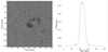 |
Fig. 1. Granule image (left panel) and the corresponding grayscale probability distribution curve (right panel). The points on the curve in the right panel are the left and right knee points of the curve. |
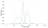 |
Fig. 2. The knee points of the grayscale probability distribution curve of five different granule observation images. The two points on the left and right of each curve are the left and right knee points of the curve. |
(3) Calculation of the values of the black and white fields: From Fig. 2, it can be observed that each curve represents the grayscale range transitioning from dark (intergranular lanes) to gray (the transition between intergranular lanes and granules, as well as other gray areas) and then to bright (granules and MBPs). The knee points on both sides of the distribution curves correspond precisely to the grayscale levels where the transitions from dark to gray and gray to bright occur. We can utilize this characteristic to remap the grayscale range of the image according to our needs, making the lanes darker and the granules brighter, which aid us in segmenting the granules more easily in the subsequent steps. We took the knee points on both sides of the curve as the black and white field values for the next step of grayscale remapping (as shown by each point on the curves in Figs. 1 and 2). In this process, we utilized the algorithm proposed by Satopaa et al. (2011) for solving this issue. Originating from the concept of curvature, the algorithm in Satopaa et al. (2011) proposes a new knee point detection method called Kneed for discrete data. This method combines angle-based (Salvador & Chan 2004; Zhao et al. 2008), Menger curvature (Tolsa 2000), exponentially weighted moving average (EWMA) (Bollinger 2002; Basseville & Nikiforov 1993; Andersen et al. 2005), and other algorithms. Kneed calculates knee points based on the convexity and concavity of the curve. Therefore, we applied the Kneed algorithm to the grayscale probability curve twice: once, by ignoring the right half of the curve and treating the remaining portion as convex to calculate the knee point on the left side; and second, by disregarding the left half and treating the curve as concave to compute the knee point on the right side.
(4) Grayscale remapping: This involves recalculating the pixel values of an image according to certain rules and mapping them to a new range, which differs from histogram equalization. This method is commonly used in various image processing software to adjust different parameters such as brightness and contrast that must be set manually. The calculation methods vary depending on the software. This study improves upon the grayscale remapping algorithm by using the knee points of the grayscale probability distribution curve to determine the black and white field parameters, which were manually specified. Additionally, the variance and mean of the image are incorporated to further constrain the mapping range. The calculation process uses the following equations:
 (3)
(3)
 (4)
(4)
![Mathematical equation: $$ \begin{aligned} O&=[E/D]^{(1/M)\times 255}+\sigma ^2, \end{aligned} $$](/articles/aa/full_html/2025/06/aa51895-24/aa51895-24-eq5.gif) (5)
(5)
where S and H represent the black and white field values, respectively, I is the input value, O is the output value, and μ and σ2 are the variance and mean. The two left and right knee points, calculated in step three, are used as the values for S and H, respectively. The parameter S defines the dark range in the image: all pixel values below this threshold in the input image are set to 0, where S ranges from 0 to H. The parameter H defines the upper threshold for brightness: all pixel values above H in the input image are set to 255, and H ranges from S to 255. M is the gray field value (also called the midtone), with a value range of 0.01–9.99 and a default value of 1.0 used to control the image’s contrast. The closer the value of M is to 0.01, the higher the image contrast; the closer it is to 9.99, the lower the image contrast. In our study, M is set to 1.
(5) Calculation of the segmentation threshold: The segmentation threshold is also derived from the probability distribution curve of the granulation grayscale values. After the image undergoes grayscale remapping, the brightness of the granules becomes more prominent, while the brightness of the background regions decreases. As mentioned above, the middle portion of the curve represents the grayscale region of the image, which serves as the boundary between the dark (background) and bright (solar granules) regions. This boundary point is precisely located at the peak of the curve. Therefore, we utilized the grayscale value corresponding to the maximum of the curve as the threshold for segmenting the solar granules. This value coincides with the intersection point between the dark and bright regions of the image after grayscale remapping. It is worth noting that the calculation of the image grayscale probability distribution curve in this step is performed after grayscale remapping.
Figure 3 shows the granule segmentation results after different processing steps on a granule image, across which BPs were not removed. It is evident that our method effectively segments granules of various sizes. Additionally, we selected three consecutive images with significant changes in imaging quality to demonstrate the adaptive segmentation capability of our method under such conditions (Fig. 4 shows the segmentation results). In Fig. 4, the imaging quality of the three images changes progressively from left to right. The middle image has the poorest quality, exhibiting excessive noise and ghosting, while the left and right images show varying degrees of radial blur from the center outward. The results indicate that our method effectively handles these conditions and achieves good segmentation performance for areas with poor quality and edge blur.
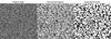 |
Fig. 3. Result of a granule observation image after grayscale remapping (left: original image; middle: grayscale remapping; right: final granule segmentation result). |
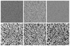 |
Fig. 4. Adaptive segmentation results of continuous granule images with sudden quality changes. The first row shows the original images, and the second row shows the corresponding segmentation results. The first and third images have radial blurring and contrast variation, while the second image has speckles and ghosting effects. |
4. Experiments with GRGP
To better demonstrate the effectiveness of GRGP for granule segmentation, we conducted tests and provided explanations using both qualitative and quantitative methods (excluding BP removal). For the quantitative aspect, we compared commonly used granule segmentation methods: adaptive MLT (Abramenko et al. 2012) (using the most effective two-level setting identified in this study) and Morphology (Deng 2015), by replicating the methods described in the original papers. Due to the lack of publicly available granule segmentation datasets and standardized algorithms for comparison, we used the same pixel-level intersection-over-union (IOU) method as Bai et al. (2023) for testing. This involves calculating the IOU at the pixel level rather than using object bounding boxes. For details, readers can refer to Bai et al. (2023). Although the final IOU values may appear low, this method is highly sensitive to pixel-level differences, effectively detecting subtle distinctions between two shapes. The ground truth (GT) images required for testing were generated through manual label. During granule labels, the granules vary in size, and some edges are difficult to define due to blurriness. Therefore, different annotators may have different interpretations of the same granule boundary. To minimize errors from manual labels, three researchers familiar with granule images independently labeled each image, resulting in three GT labels per image. The final IOU value for each tested method on a given image was calculated as the average IOU between the segmentation result and these three GT images. A total of 60 images were tested, randomly divided into three groups, each group containing 20 granule images and their 60 manually labeled GT images. The average IOU value for each tested method within a group was considered the result. The test results for GRGP, MLT, and Morphology are shown in Table 1. The table clearly shows that GRGP outperforms the other two methods in all three groups, with IOU values closer to 1 indicating better performance.
Comparison of IOU results between GRGP and other methods on three groups of test images.
To qualitatively compare the granule segmentation capabilities of GRGP, Fig. 5 presents the segmentation results for the three images using these methods. The imaging conditions of each image are different. From left to right, each column shows the original image, manual labeling, GRGP, adaptive MLT, and Morphology. The number below each segmented image indicates the detected granule count. Except for manual labeling, all the segmented images include BPs and sunspots, which can lead to misidentifications by all methods when such features are present. We note that manual labeling is based on manually labeled images. Due to the indistinct boundaries of some granules–which can appear even more ambiguous when the image is magnified for annotation, as the richer details make the boundaries harder to discern–the boundary definitions may exhibit some discrepancies. From Fig. 5, it is evident that both MLT and Morphology show significant segmentation deficiencies. While MLT can segment most granules, its ability to delineate the boundaries of large granules is suboptimal, leading to under-segmentation and uneven edges. In some cases, granules are over-segmented. Overall, Morphology outperforms MLT slightly, particularly in segmenting small granules, but both methods perform similarly on large granules. Similar to the other two methods, GRGP encounters under-segmentation when granule edges are severely blurred or when BPs adhere to granules. Nevertheless, GRGP’s results overall are closer to those of manual labeling. It segments all granules more effectively with better control over edge boundaries. Additionally, the number of granules detected by GRGP is closer to that obtained by manual labeling compared to the other two methods.
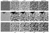 |
Fig. 5. Comparison of granule segmentation results among GRGP, MLT, and Morphology. The first column shows the original images; the second column presents the manually labeled granules; and the third to fifth columns display the segmentation results obtained by different methods without removing BPs and sunspots. The numbers below each image starting from the second column represent the number of granules in the corresponding image. |
5. Data processing, analysis, and discussion of the results
We used the GRGP algorithm method to identify the granules in two sets of continuously observed images from BBSO, aiming to study the variation characteristics of the three size-scale groups of granules in the quiet region and the active region. The detailed data processing and computational procedures are outlined in the following steps.
(1) Solar granule segmentation: The original solar granule observation images have a size of 2043 × 2043 pixels, with each pixel representing 0.0342 arcseconds. There is a black border of 200 pixels along the edges of the images. After cropping the black border, the image size becomes 1643 × 1643 pixels. We utilized the GRGP granule segmentation algorithm to segment all granules in each frame of the images. Both datasets contain some BPs, and the active region data also includes sunspots. We applied BP (Bai et al. 2023; Yang et al. 2023) and sunspot segmentation algorithms (Gong et al. 2023) to remove both these features from each frame.
(2) Calculating the size of granules: Following the research of Liu et al. (2021), we considered each granule as circular and measured its size by calculating the equivalent diameter. This step required segmenting and measuring the size of all granules in each frame.
(3) Calculating the relative proportion of granule numbers: we determined the size of all granules in each frame following step 2. Then, we classified the granules into three size ranges (i.e., less than 265 km, between 265 km and 1420 km, and greater than 1420 km) and calculated the relative proportion of granule numbers within each range for every frame. The relative proportion, rather than the absolute number, was used because active regions contain sunspot areas that occupy a certain amount of space, potentially affecting the granule number statistics in those regions. To ensure the accuracy of the analysis, granules smaller than 50 km and larger than 3500 km were excluded. Hereafter, granules within the three size ranges are referred to as d1 (d1 ≤ 265 km), d2 (265 km < d2 < 1420 km), and d3 (d3 ≥ 1420 km). The term “granule number” specifically refers to the relative proportion of granules.
Through the above three steps, we obtained the variation data of the number of granules within three granule size intervals in the quiet region and the active region. Since our data is based on image frames and the time intervals between each in the active region and the quiet region are not the same (as described in Sect. 2). For clarity and ease of comparison, we take the frame as the time unit on the X-axis and the number of granules of three sizes in each frame as the Y-axis to draw the evolution curves of the number of granules in the quiet region and the active region at three size scales (d1 – d3). Figures 6–8 show the comparative evolution curves of the proportion of the number of granules from d1 to d3, respectively. In the figures, the purple curve represents the quiet region, and the orange represents the active region.
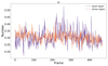 |
Fig. 6. Dynamic variation curve of the relative proportion of the number of granules at the d1 size scale. Red represents the active region, and blue represents the quiet region. In this granule size interval, the two curves overlap. |
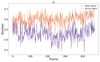 |
Fig. 7. Dynamic variation curve of the relative proportion of the number of d2-sized granules. Red represents the active region, while blue represents the quiet region. In this granule size interval, the curve of the active region is above that of the quiet region. |
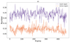 |
Fig. 8. Dynamic variation curve of the relative proportion of the number of d3-sized granules. Red represents the active region, while blue represents the quiet region. In this granule size interval, the curve of the active region is below that of the quiet region. |
From Figs. 6 to 8, we can clearly observe the continuous variation in the numbers of granules across the three size ranges in the quiet and active regions. To better analyze the fluctuations and trends in granule numbers, we calculated the upper quartile (75%), lower quartile (25%), and the interquartile range (IQR) for each set of variation data. The upper and lower quartiles were used to represent the upper and lower fluctuation bounds of each variation curve. Details are provided in Table 2. Next, we analyzed the variation in granule numbers by combining the information from Figs. 6 to 8 and Table 2.
Range and difference of the fluctuation curves of the relative proportion of the number of granules at three different size scales.
As can be clearly seen from Figs. 6 to 8, there are significant differences in the dynamic changes in the number of granules between the quiet region and the active region. In the d1 interval, the two variation curves overlap. However, the fluctuation amplitude in the quiet region is notably larger than that in the active region. The difference between the upper and lower quartiles for d1 in Table 2 also reflects this point: 0.06 for the quiet region and 0.04 for the active region. Nevertheless, within this granule size scale interval, the baseline (equilibrium position) of the fluctuation curves is essentially the same in both the quiet and active regions (approximately 0.30), with both regions oscillating around this baseline. This indicates that, for granules of the d1 scale, the baseline of their number fluctuations is nearly identical, regardless of whether they are in the quiet region or the active region. In terms of fluctuation amplitude, the quiet region exhibits slightly larger variations compared to the active region.
Within the d2 interval, the two curves no longer overlap. The baseline of the fluctuation curve in the active region is approximately 0.6, while that in the quiet region is around 0.45. The baseline in the active region is higher than that in the quiet region, and both regions oscillate around their respective baselines. However, the fluctuation amplitude in the quiet region (0.08) is larger than that in the active region (0.06). As can be seen in Table 2, within this interval, the lower and upper quartiles in the quiet region are 0.42 and 0.50 respectively, with a difference of 0.08. In the active region, they are 0.58 and 0.84 respectively, with a difference of 0.06. This indicates that, within the granule size interval of d2, the number of granules in the active region is generally greater than that in the quiet region, and this state varies within a relatively small fluctuation range. In contrast, the quiet region exhibits larger fluctuations.
Within the d3 interval, the two curves are completely separated, oscillating around their respective baselines. In this interval, the baseline of the active region is approximately 0.225, while that of the quiet region is around 0.084. In contrast to the d2 interval, the baseline of the quiet region is higher than that of the active region. The amplitude of fluctuation within the active region is substantially less than that in the quiet region, signifying that the quantity of large granules at the d3 scale in the active region is inferior to that in the quiet region. Nevertheless, the disparities between the lower and upper quartiles in both the quiet region and the active region are congruent, and their magnitudes of fluctuation are nearly equivalent.
Based on the analysis above, it can be concluded that the changes in the number of granules at three size scales exhibit distinct characteristics in both the active and the quiet region. Generally speaking, granules of size d2 constitute the vast majority in both regions, followed by those of size d1, while granules of size d3 are the least numerous. It is evident that large-scale granules are relatively scarce in both the quiet region and the active region. Although the proportional distribution of granules across the three size scales is consistent in both regions (i.e., d2 > d1 > d3), the active region has a relatively larger number of d2-scale granules and fewer d3-scale granules. The primary reason for this may be that granules in magnetic regions are smaller, leading to an increase in the proportion of d2-scale granules and a decrease in the proportion of d3-scale granules when a magnetic field is present in the active region (Roudier et al. 2020). Another possible reason is that, in both regions, d3-scale granules are more unstable under the influence of convection and tend to decompose continuously and steadily into smaller-scale granules within a short period. Specifically, large-scale granules in the active region decompose at a faster rate, with some unstable d3-scale granules breaking down into d2-scale granules. These characteristics further illustrate that, in the active region, the decomposition of large granules–driven by magnetic fields and convective instability–results in energy being transferred to smaller granules at a faster rate. This indicates a more rapid cascading process in the active region (Liu et al. 2021). This accelerated cascading process may play a positive role in the formation of sunspots; conversely, the process of sunspot formation may also enhance the cascading process of granules.
Above, we have visually analyzed the variation curves of granule numbers in different size ranges for the quiet and active regions. However, these curves alone do not provide sufficient information. Therefore, we applied Variational Mode Decomposition (VMD) (Dragomiretskiy & Zosso 2014) to decompose these curves, extract the characteristic information of the signal across different frequency ranges, and uncover more hidden details. VMD is an adaptive, completely non-recursive modal decomposition and signal processing method. Its adaptability is reflected in the ability to determine the number of modal components for a given sequence based on the actual data. It can also adaptively match the optimal center frequency and finite bandwidth for each mode and effectively separate the intrinsic mode functions (IMFs). This enables the frequency-domain partitioning, ultimately providing the effective components of the given signal and yielding the optimal solution to the variational problem. The result of VMD decomposition is that the original signal can be represented as a sum of various modal components. The original signal, in turn, can be reconstructed from the modal functions obtained through this process. The decomposition results from the VMD reveal the underlying structure of different frequency components within the signal, thereby aiding in the understanding of the signal’s composition and its variations on long, medium, and short-term timescales.
Calculation results of the correlation coefficients of the five IMF components among Q_d1, Q_d2 and Q_d3.
The number of modal components required for VMD decomposition can be determined using three methods: spectral analysis, reconstruction error analysis, and energy criteria. In this study, we determined the number of components by using spectral analysis to identify the significant frequency components present in the curves. Through analysis and observation, we identified four to six significant frequency components in the curves. Therefore, the final decomposition number was set to five, meaning each curve was decomposed into five IMFs, where IMF1 to IMF5 represent the frequency components from low to high frequency. VMD also requires a penalty factor to control the bandwidth of each IMF component. The typical bandwidth limit is empirically set to 1.5–2.0 times the length of the sampling points. In this study, we used twice the sampling point length, so the penalty factor was set to 2 × 469 = 938.
After performing VMD decomposition on the granule number variation curves across the three size scales in the quiet and active regions, we obtained five IMF components for each curve. For convenience in later descriptions, the three different granule size curves for the quiet region are denoted Q_d1, Q_d2, and Q_d3, while those for the active region are denoted A_d1, A_d2, and A_d3. Here, di (i = 1, 2, 3) refers to granules of size di (i = 1, 2, 3). Figures 9 and 10 show the VMD decomposition results of the A_d1 and Q_d3 curves among the six total curves.
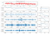 |
Fig. 9. Results of decomposing the A_d1 curve into five IMFs using VMD. The first column shows, from top to bottom, the original signal and the five IMF components in order of increasing frequency (IMF1 to IMF5); the second column shows the central frequency of each component. |
The first row in the first column of Figs. 9 and 10 shows the original granule number variation curve. The first column, rows two to six display the five IMF components (IMF1 to IMF5) obtained from the VMD decomposition of the curve. The second column shows the corresponding center frequency for each IMF component. The five IMF components (IMF1 to IMF5) are the result of decomposing the original variation curve into frequency components from low to high. Each IMF corresponds to the frequency-based signal decomposition characteristics. From Figs. 9 and 10, it can be observed that the IMF1 waveform captures the lowest frequency component of the variation curve. The waveforms of IMF2 to IMF5 progressively become more regular and uniform, with IMF5 having the highest frequency and the smoothest waveform. These IMF components reflect the variation characteristics of granule numbers at different timescales, and together they form a comprehensive picture of granule number variation. Among these features, the combination of high-frequency and low-frequency components may jointly influence the short-term behavior of granule numbers, with potential interactions between different components. For example, the mid-frequency component may be modulated by the low-frequency long-term trend, while the high-frequency component may be amplified or attenuated due to the enhancement or damping of mid-frequency fluctuations. To further investigate these interactions, we computed the correlation coefficient matrices for the IMF component characteristic data among the three curves within each region. With three curves in each region, three correlation coefficient matrices were calculated for each region, resulting in a total of six correlation coefficient matrices for both regions. Tables 3–6 present the relevant calculation results with the data rounded to one decimal place.
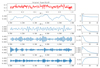 |
Fig. 10. Results of decomposing the Q_d3 curve into five IMFs using VMD. The first column shows, from top to bottom, the original signal and the five IMF components in order of increasing frequency (IMF1 to IMF5); the second column shows the central frequency of each component. |
The correlation coefficient ranges from −1 to 1. A value of 0 indicates that the two variables are completely uncorrelated. The closer the coefficient is to 1, the stronger the positive correlation; the closer it is to −1, the stronger the negative correlation. Through calculations, we find that there is a high correlation between the IMF components of the granule number variation curves of different scales within each region.
In the quiet region, the IMF components of the quantity variation curves for different granule size scales exhibit high positive or negative correlation characteristics. As shown in Tables 3 and 4, except for IMF2, which has a relatively low value of −0.4, the IMF components between Q_d1 and Q_d2 exhibit very strong negative correlations, with most reaching −0.8, and IMF1 even attaining −0.9. Similarly, the IMF components between Q_d2 and Q_d3 also show relatively high negative correlations, except for IMF2 and IMF3, which have lower correlation values of −0.2 and −0.4, respectively. This indicates that the quantity variations of d1 and d2 in the quiet region exhibit strong negative correlations across different timescales, although the correlation is slightly weaker at medium to long timescales. An increase in the number of d2 granules corresponds to a descrease in d1 granules, and vice versa. There is a similar relationship between d2 and d3; however, this characteristic is mainly observed on long- and short-term timescales represented by low and high-frequency components; moreover, the negative correlation between d2 and d3 is weaker compared to that between d1 and d2. In contrast, as seen in Table 3, Q_d1 and Q_d3 are positively correlated in IMF1 and IMF5, albeit with moderate strength. There is no significant correlation among other IMF components. This suggests that in the quiet region, the granule quantities at the d1 and d3 scales exhibit some degree of positive correlation on long- and short-term timescales.
Calculation results of the correlation coefficients of the five IMF components among Q_d2 and Q_d3.
The correlation characteristics of the IMF components in the active region share similarities with those in the quiet region but also exhibit notable differences. Overall, the correlations between the IMFs in the active region are more pronounced. As shown in Tables 5 and 6, the IMF components between A_d1 and A_d2, as well as A_d2 and A_d3 exhibit very high negative correlations from IMF1 to IMF5. In particular, the correlation coefficients between A_d1 and A_d2 reach −0.9 for all components except IMF3. The distribution of the correlation coefficients shows a consistent pattern: the correlation coefficient for IMF3 is relatively lower, while those for the other components are higher. This indicates that strong negative correlations exist at both low and high-frequency timescales, whereas the negative correlation at mid-frequency timescales is relatively weaker. Based solely on the correlation coefficients, the negative correlation between A_d1 and A_d2 is stronger than that between A_d2 and A_d3. The average correlation coefficient across the five IMFs is 0.8 for the former and 0.68 for the latter.
Calculation results of the correlation coefficients of the five IMF components among A_d1, A_d2 and A_d3.
Calculation results of the correlation coefficients of the five IMF components among A_d2 and A_d3.
On the other hand, unlike in the quiet region, the IMF components between A_d1 and A_d3 show positive correlations, with the correlation coefficients exhibiting a pattern of being lower in the middle and higher at both ends. This indicates that, when the number of small-scale granules increases or decreases, the number of medium-scale granules necessarily decreases or increases in the active region. Similarly, when the number of medium-scale granules increases or decreases, the number of large-scale granules necessarily decreases or increases. However, the variation trends of the small-scale and large-scale granule quantities are consistent. Regarding the timescales of granule quantity variations, the influence between different granule sizes is stronger at long-term and short-term timescales than at mid-term timescales. For example, localized rapid convection may accelerate granule fragmentation and thereby influence the rapid changes in the quantities of granules of different sizes on short timescales. Additionally, the stronger magnetic field concentrations or sunspots (and other long-period solar activities) potentially present in the active region may also affect the long-term variations in granule quantities and the predominant granule size. The higher correlations between different frequency components in the active region suggest that, compared to the quiet region, the processes of large granules breaking into medium granules and medium granules breaking into small granules–likely driven by stronger magnetic field concentrations and convective instabilities–are more stable and rapid in the active region, with d3 granules decomposing at the fastest rate. Consequently, the granule morphology in the active region is predominantly characterized by small and medium-sized scales. Specifically, d3 granules (large granules) continuously and rapidly decompose, preventing their numbers from remaining at a relatively high level. Meanwhile, the decomposition rate of medium-sized granules (d2) significantly lags behind that of large granules (d3), leading to an increase in the number of d2 granules (medium-sized granules). This phenomenon is reflected in the observation that the number of d2 granules in the active region is notably higher than in the quiet region (as can be seen in Fig. 7), where the curve for the active region is higher than that for the quiet region. In both regions, the decomposition rates of d2 and d1 granules do not change significantly. Thus, the increase in d1 granule numbers is not pronounced, although the active region exhibits greater stability.
In general, the changes in the number of granules of different sizes in the quiet region and the active region have their own distinct characteristics. Overall, the changes in the number of d1, d2, and d3 granules in the quiet and, especially, in the active region can always maintain a relatively stable state without drastic fluctuations. Among these, the medium-sized granules account for the largest proportion in quantity, followed by the small-sized granules. The large-sized granules are the fewest. However, compared to the quiet region, the active region has a higher proportion of granules overall but a lower proportion of large-sized granules. During changes in granule numbers, the decomposition process in the active region is more stable and rapid, while in the quiet region it is more volatile and slower. In the active region, the decomposition process of large-sized granules is faster and more stable. Although the decomposition speeds of medium-sized and small-sized granules do not change much compared to those in the quiet region, they are more stable. There is a distinct correlation between the changes in the number of granules within different timescale ranges (i.e., different frequencies) in the active region, especially on long-term (i.e., low-frequency) and short-term (i.e., high-frequency) timescales. In the quiet region, it is relatively weaker, but there is still a very obvious correlation on long-term and short-term scales. This indicates that both long-period solar activity and local rapid changes have a greater influence on the number of granules. This verifies the findings of Ballot et al. (2021) from another perspective: during the sunspot activity cycle, the size and density of granulation tissue are affected. This is a noteworthy phenomenon, but the reasons behind it nonetheless require further in-depth research.
6. Conclusions
This study investigated the dynamic and continuous variation characteristics of the number of solar photospheric granule groups with equivalent diameters (d) in three different size scales–d1 (d1 ≤ 265 km), d2 (265 km < d2 < 1420 km), and d3 (d3 ≥ 1420 km) in the solar photosphere–comparing local active regions and quiet regions. To achieve this, a granule segmentation method named GRGP is developed, which combines grayscale remapping with the knee points of the grayscale probability distribution curve. Compared to other mainstream methods, GRGP demonstrates excellent control over granule edges, significantly improving segmentation accuracy for granules with blurred edges. It effectively handles granule segmentation in continuous images with fluctuating quality. The method also performs well on data from both the BBSO and NVST telescopes.
Based on the GRGP granule segmentation method, we segmented the granules from continuous observational data (i.e., a total of 938 images) of a quiet and an active region. Then, we counted the proportion of the number of granules within each frame according to their equivalent diameters. Taking the frame as the X-axis and the number as the Y-axis, we plotted the variation curves of the proportion of the number of granules within three size scales in the two regions. Through comparative analysis of these curves, we find that the decomposition of granules in the active region is faster and more stable, especially for the granules at the d3 scale. Additionally, in both regions, the granules at the d2 scale are the most abundant, and the number of granules at the d3 scale is the least numerous. However, in the active region, the proportion of d2 granules is larger, while that of d3 granules is smaller. To gain a deeper understanding of the variation characteristics and interrelationships of the number of granules at different size scales in these two regions on different frequencies (i.e., timescales), we further decomposed each variation curve into five IMF variation characteristic components using VMD. These five IMFs, from IMF1 to IMF5, represent different frequency components of the original data from high to low frequencies. We also calculated the correlation coefficient matrix of the IMF components of all curves. Among the granules of different size scales within each region, changes in the numbers of d1 and d2 granules, as well as d2 and d3 granules are negatively correlated at both low and high frequencies, while changes in d1 and d3 granules are positively correlated. This characteristic is more pronounced in the active region. This indicates that in both regions, there is a higher correlation between low frequencies (i.e., long-term timescales) and high frequencies (i.e., short-term timescales) in the changes of the number of granules. The long-term timescale represents gradual variations in the number of granules, while the short-term timescale represents rapid variation. As mentioned above, long-term timescale changes may be influenced by the sun’s long-term periodic activity, while short-term changes are affected by both these long-term solar activities and local rapid changes. Therefore, the long-term periodic activities of the sun and local rapid changes (e.g., convection) are more likely to affect the number of granules of different sizes, especially in the active region. Lastly, we find that the decomposition of granules in the active region is faster and more stable, especially for those of size d3. These features may be related to the magnetic fields of active regions, sunspots, and other solar activities.
In summary, our study reveals that the granule activities in active and quiet regions exhibit completely distinct characteristics. In different regions, variations in the quantities of granules of different sizes show certain correlations. Granule activity in active regions is more intense, particularly for large granules. The decomposition of granules is also more stable and rapid in active regions. Magnetic fields, long-term solar activity, and short-term localized dynamics may have a certain impact on the quantities of granules at different scales. The underlying physical mechanisms behind these characteristics require further in-depth investigation and will be the focus of our future research efforts.
Acknowledgments
We gratefully acknowledge the use of data from the Goode Solar Telescope (GST) of the Big Bear Solar Observatory (BBSO). BBSO operation is supported by US NSF AGS2309939 and AGS1821294 grants and New Jersey Institute of Technology. GST operation is partly supported by the Korea Astronomy and Space Science Institute and the Seoul National University. The data used in this paper were obtained with the New Vacuum Solar Telescope in Fuxian Solar Observatory of Yunnan Astronomical Observatory, CAS. This work was funded by the National Natural Science Foundation of China (12463010).
References
- Abramenko, V. I., Yurchyshyn, V. B., Goode, P. R., Kitiashvili, I. N., & Kosovichev, A. G. 2012, ApJ, 756, L27 [NASA ADS] [CrossRef] [Google Scholar]
- Andersen, D. G., Balakrishnan, H., Kaashoek, M. F., & Rao, R. N. 2005, in Proceedings of the 2nd conference on Symposium on Networked Systems Design& Implementation-Volume 2, 115 [Google Scholar]
- Bai, H., Yang, P., Zhao, L., et al. 2023, ApJ, 956, 62 [Google Scholar]
- Ballot, J., Roudier, T., Malherbe, J. M., & Frank, Z. 2021, A&A, 652, A103 [NASA ADS] [CrossRef] [EDP Sciences] [Google Scholar]
- Basseville, M., & Nikiforov, I. V. 1993, Detection of Abrupt Changes: Theory and Application (Prentice hall Englewood Cliffs), 104 [Google Scholar]
- Bollinger, J. 2002, Bollinger on Bollinger bands (McGraw-Hill New York) [Google Scholar]
- Bovelet, B., & Wiehr, E. 2001, Sol. Phys., 201, 13 [NASA ADS] [CrossRef] [Google Scholar]
- Bovelet, B., & Wiehr, E. 2007, Sol. Phys., 243, 121 [Google Scholar]
- Cao, W., Gorceix, N., Coulter, R., et al. 2010, Astron. Nachr., 331, 636 [Google Scholar]
- Chen, H., & Wu, R. 2023, arXiv e-prints [arXiv:2211.08113] [Google Scholar]
- Cuicui, H., Xia, J., Yunfei, Y., et al. 2016, Chinese Science Bulletin, 61, 881 [Google Scholar]
- Del Moro, D. 2004, A&A, 428, 1007 [NASA ADS] [CrossRef] [EDP Sciences] [Google Scholar]
- Deng, L. 2015, in Proceeding of the 11th World Congress on Intelligent Control and Automation, 3364 [Google Scholar]
- Díaz Castillo, S., Asensio Ramos, A., Fischer, C., & Berdyugina, S. 2022, Front. Astron. Space Sci., 9, 896632 [Google Scholar]
- Dragomiretskiy, K., & Zosso, D. 2014, IEEE Trans. Signal Process., 62, 531 [CrossRef] [Google Scholar]
- Gong, X., Zhong, L., & Rao, C. 2023, A&A, 670, A132 [NASA ADS] [CrossRef] [EDP Sciences] [Google Scholar]
- Goode, P. R., & Cao, W. 2012, Proc. SPIE, 8444, 844403 [Google Scholar]
- Hirzberger, J., Bonet, J., Vázquez, M., & Hanslmeier, A. 1999, ApJ, 515, 441 [NASA ADS] [CrossRef] [Google Scholar]
- Javaherian, M., Safari, H., Amiri, A., & Ziaei, S. 2014, Sol. Phys., 289, 3969 [Google Scholar]
- Lemmerer, B., Hanslmeier, A., Muthsam, H., & Piantschitsch, I. 2017, A&A, 598, A126 [NASA ADS] [CrossRef] [EDP Sciences] [Google Scholar]
- Liu, Y., Jiang, C., Yuan, D., et al. 2021, ApJ, 923, 133 [Google Scholar]
- Oba, T., Iida, Y., & Shimizu, T. 2020, ApJ, 890, 141 [NASA ADS] [CrossRef] [Google Scholar]
- Rieutord, M., Roudier, T., Roques, S., & Ducottet, C. 2007, A&A, 471, 687 [NASA ADS] [CrossRef] [EDP Sciences] [Google Scholar]
- Roudier, T., & Muller, R. 1986, Sol. Phys., 107, 11 [NASA ADS] [CrossRef] [Google Scholar]
- Roudier, T., Malherbe, J., Gelly, B., et al. 2020, A&A, 641, A50 [NASA ADS] [CrossRef] [EDP Sciences] [Google Scholar]
- Salvador, S., & Chan, P. 2004, in 16th IEEE International Conference on Tools with Artificial Intelligence (IEEE), 576 [Google Scholar]
- Satopaa, V., Albrecht, J., Irwin, D., & Raghavan, B. 2011, in 2011 31st International Conference on Distributed Computing Systems Workshops, 166 [Google Scholar]
- Stein, R. F., & Nordlund, A. 1998, ApJ, 499, 898 [Google Scholar]
- Tolsa, X. 2000, Proc. Am. Math. Soc., 128, 2111 [Google Scholar]
- Yang, P., Bai, H., Zhao, L., et al. 2023, A&A, 677, A121 [NASA ADS] [CrossRef] [EDP Sciences] [Google Scholar]
- Zhao, Q., Hautamaki, V., & Fränti, P. 2008, in International Conference on Advanced Concepts for Intelligent Vision Systems (Springer), 664 [Google Scholar]
All Tables
Comparison of IOU results between GRGP and other methods on three groups of test images.
Range and difference of the fluctuation curves of the relative proportion of the number of granules at three different size scales.
Calculation results of the correlation coefficients of the five IMF components among Q_d1, Q_d2 and Q_d3.
Calculation results of the correlation coefficients of the five IMF components among Q_d2 and Q_d3.
Calculation results of the correlation coefficients of the five IMF components among A_d1, A_d2 and A_d3.
Calculation results of the correlation coefficients of the five IMF components among A_d2 and A_d3.
All Figures
|
Fig. 1. Granule image (left panel) and the corresponding grayscale probability distribution curve (right panel). The points on the curve in the right panel are the left and right knee points of the curve. |
| In the text | |
|
Fig. 2. The knee points of the grayscale probability distribution curve of five different granule observation images. The two points on the left and right of each curve are the left and right knee points of the curve. |
| In the text | |
|
Fig. 3. Result of a granule observation image after grayscale remapping (left: original image; middle: grayscale remapping; right: final granule segmentation result). |
| In the text | |
|
Fig. 4. Adaptive segmentation results of continuous granule images with sudden quality changes. The first row shows the original images, and the second row shows the corresponding segmentation results. The first and third images have radial blurring and contrast variation, while the second image has speckles and ghosting effects. |
| In the text | |
|
Fig. 5. Comparison of granule segmentation results among GRGP, MLT, and Morphology. The first column shows the original images; the second column presents the manually labeled granules; and the third to fifth columns display the segmentation results obtained by different methods without removing BPs and sunspots. The numbers below each image starting from the second column represent the number of granules in the corresponding image. |
| In the text | |
|
Fig. 6. Dynamic variation curve of the relative proportion of the number of granules at the d1 size scale. Red represents the active region, and blue represents the quiet region. In this granule size interval, the two curves overlap. |
| In the text | |
|
Fig. 7. Dynamic variation curve of the relative proportion of the number of d2-sized granules. Red represents the active region, while blue represents the quiet region. In this granule size interval, the curve of the active region is above that of the quiet region. |
| In the text | |
|
Fig. 8. Dynamic variation curve of the relative proportion of the number of d3-sized granules. Red represents the active region, while blue represents the quiet region. In this granule size interval, the curve of the active region is below that of the quiet region. |
| In the text | |
|
Fig. 9. Results of decomposing the A_d1 curve into five IMFs using VMD. The first column shows, from top to bottom, the original signal and the five IMF components in order of increasing frequency (IMF1 to IMF5); the second column shows the central frequency of each component. |
| In the text | |
|
Fig. 10. Results of decomposing the Q_d3 curve into five IMFs using VMD. The first column shows, from top to bottom, the original signal and the five IMF components in order of increasing frequency (IMF1 to IMF5); the second column shows the central frequency of each component. |
| In the text | |
Current usage metrics show cumulative count of Article Views (full-text article views including HTML views, PDF and ePub downloads, according to the available data) and Abstracts Views on Vision4Press platform.
Data correspond to usage on the plateform after 2015. The current usage metrics is available 48-96 hours after online publication and is updated daily on week days.
Initial download of the metrics may take a while.