| Issue |
A&A
Volume 698, June 2025
|
|
|---|---|---|
| Article Number | A29 | |
| Number of page(s) | 6 | |
| Section | Cosmology (including clusters of galaxies) | |
| DOI | https://doi.org/10.1051/0004-6361/202451362 | |
| Published online | 26 May 2025 | |
A new candidate quasar strongly lensed by the galaxy cluster WHJ0400-27 with an 18″ image separation
1
Department of Physics and Earth Science, University of Ferrara, via Saragat 1, I-44122 Ferrara, Italy
2
INAF – OAS, Osservatorio di Astrofisica e Scienza dello Spazio di Bologna, via Gobetti 93/3, I-40129 Bologna, Italy
3
INAF – Osservatorio Astronomico di Capodimonte, Salita Moiariello 16, I-80131 Napoli, Italy
4
Dipartimento di Fisica, Università degli Studi di Milano, via Celoria 16, I-20133 Milano, Italy
5
INAF – IASF Milano, via A. Corti 12, I-20133 Milano, Italy
6
Departamento de Física Moderna, Instituto de Fisica de Cantabria, Avd. Los Castros 48, 39005 Santander, Spain
7
Università di Firenze, Dipartimento di Fisica e Astronomia, via G. Sansone 1, 50019 Sesto F.no, Firenze, Italy
8
INAF – Osservatorio Astrofisico di Arcetri, Via Largo E. Fermi 5, 50125 Firenze, Italy
9
Zentrum für Astronomie, Universität Heidelberg, Philosophenweg 12, D-69120 Heidelberg, Germany
10
ITP, Universität Heidelberg, Philosophenweg 16, D-69120 Heidelberg, Germany
11
INAF – Osservatorio Astronomico di Padova, vicolo dell’Osservatorio 5, I-35122 Padova, Italy
12
Università di Salerno, Dipartimento di Fisica “E.R. Caianiello”, Via Giovanni Paolo II 132, I-84084 Fisciano (SA), Italy
13
University of Trento, Via Sommarive 14, I-38123 Trento, Italy
14
INFN – Gruppo Collegato di Salerno – Sezione di Napoli, Dipartimento di Fisica “E.R. Caianiello”, Università di Salerno, via Giovanni Paolo II, 132, I-84084 Fisciano (SA), Italy
⋆ Corresponding author; This email address is being protected from spambots. You need JavaScript enabled to view it.
Received:
3
July
2024
Accepted:
9
April
2025
Abstract
Context. Time-delay cosmography (TDC) using quasi-stellar objects (QSOs) multiply lensed by galaxies has recently emerged as an independent and competitive tool for measuring the value of the Hubble constant. Lens galaxy clusters hosting multiply imaged QSOs, when coupled with an accurate and precise knowledge of their total mass distribution, are equally powerful cosmological probes. However, fewer than ten such systems have been identified to date.
Aims. Our study aims to expand the limited sample of cluster-lensed QSO systems by identifying new candidates within rich galaxy clusters.
Methods. We started with a sample of approximately 105 galaxy cluster candidates from Dark Energy Survey and Wide-field Infrared Survey Explorer imaging data, along with a pure catalogue of over one million QSOs from Gaia DR3. We cross-correlated these datasets to identify lensed QSO candidates near the cores of massive galaxy clusters.
Results. Our search detected three lensed double candidates across an area of ≈5000 sq degree. In this work, we focus on the best candidate – a double QSO with a Gaia-based redshift of 1.35, projected behind the moderately rich cluster WHJ0400-27 at zphot = 0.65. Based on a first spectroscopic follow-up study, we confirm the two QSOs at z = 1.345 with indistinguishable spectra, and a brightest cluster galaxy at z = 0.626. These observations support the strong lensing nature of this system, though some tension arises when the cluster mass from the preliminary lens model is compared to other mass proxies. We also considered whether such a system could be a rare physical association of two distinct QSOs separated by a projected physical distance of ≈150 kpc. If further spectroscopic observations confirm its lensing nature, such a rare lens system would exhibit one of the largest image separations observed to date (Δϑ = 17.8″) and would enable interesting TDC applications.
Key words: gravitational lensing: strong / galaxies: clusters: general / quasars: general / cosmology: observations
© The Authors 2025
 Open Access article, published by EDP Sciences, under the terms of the Creative Commons Attribution License (https://creativecommons.org/licenses/by/4.0), which permits unrestricted use, distribution, and reproduction in any medium, provided the original work is properly cited.
This article is published in open access under the Subscribe to Open model. This email address is being protected from spambots. You need JavaScript enabled to view it. to support open access publication.
1. Introduction
The Hubble constant (H0) stands as a pivotal cosmological parameter defining the dimensions, age, and expansion rate of the Universe. The increased precision in its determination has revealed significant discrepancies between estimates derived from observations in the local Universe and those derived from early Universe probes (Verde et al. 2019; Moresco et al. 2022). Independent and complementary techniques for measuring the value of H0 are crucial to assessing this tension, as they may point to new physics beyond the standard cosmological model.
Refsdal (1964) predicted that time delays between multiple images of strongly lensed supernovae (SNe) or variable sources such as quasi-stellar objects (QSOs) could offer a novel method for measuring the value of H0. Since then, time-delay cosmography (TDC) has matured into a technique that provides competitive estimates of this parameter. In particular, QSOs strongly lensed by galaxies have been utilised by the H0 Lenses in COSMOGRAIL’s Wellspring (H0LiCOW) program (Suyu et al. 2017) to measure H0 with 2.4% precision through a joint analysis of six gravitationally lensed QSOs (Wong et al. 2020), each providing measurements with precisions ranging from 3.6 to 9.3%.
On the other hand, while largely unexploited to date, the use of time-varying sources strongly lensed by galaxy clusters as a complementary technique has recently proven its sheer potential. SN Refsdal, discovered by Kelly et al. (2015) to be strongly lensed by the galaxy cluster J1149.5+2223 in the MAssive Cluster Survey (MACS), led Grillo et al. (2024) to infer the value of H0 with a 6% (statistical plus systematic) uncertainty. They used a full strong-lensing (SL) analysis, which included the measured time delays between the multiple SN images and their associated uncertainties (see also Grillo et al. 2018, 2020). This study also demonstrated that time delays in lens galaxy clusters are a valuable and complementary tool for measuring both H0 and the geometry (Ωm, ΩDE, and w) of the Universe, by exploiting the observed positions of other multiply lensed sources at different redshifts. These allow for a significant reduction in the mass-sheet degeneracy, which plagues TDC with galaxy-scale lens systems (Birrer et al. 2016; Grillo et al. 2020; Moresco et al. 2022).
As estimated by Treu et al. (2022), a sample of about 40 lensed QSOs or SNe could produce a H0 measurement with a precision of approximately 1%. This can be extremely relevant for assessing H0 tension. However, fewer than ten QSOs strongly lensed by galaxy clusters have been discovered to date (Inada et al. 2003, 2006; Dahle et al. 2013; Shu et al. 2018, 2019; Martinez et al. 2023; Napier et al. 2023). Expanding the sample is therefore of paramount importance and can guide the search for such rare systems in upcoming wide-field surveys, such as Euclid (Euclid Collaboration: Adam et al. 2019) and the Vera C. Rubin Large Synoptic Survey Telescope (LSST; Ivezić et al. 2019). Other studies (e.g., Dutta et al. 2024) use QSOs strongly lensed by galaxy clusters to probe the circumgalactic medium and investigate the distribution and coherence of metal-enriched gaseous structures.
As part of a search for Gaia QSOs gravitationally lensed by galaxy clusters, we present the discovery of a QSO pair (zGaia ≃ 1.35) potentially lensed by a relatively rich Dark Energy Survey (DES) galaxy cluster at z ≃ 0.63. If confirmed, the image separation of ∼18″ would make it one of the largest separation systems among lensed QSOs known to date. We also considered the possibility that this system is a dual active galactic nucleus (AGN) (e.g. Hennawi et al. 2006; Mannucci et al. 2023). Such a system is often considered a candidate for supermassive black-hole mergers, making it very rare given the remarkable similarities between the two QSO spectra. The data and the implemented search algorithm used in our study are detailed in Sect. 2. In Sect. 3 we present the follow-up ground-based spectroscopy, which makes this candidate a likely gravitationally lensed QSO, along with a preliminary SL model of the lens galaxy cluster. In Sect. 4 we discuss the challenges posed by the SL interpretation. In Sect. 5 we summarise our findings for and against the SL scenario.
Throughout the paper, we assume a flat Lambda cold dark matter cosmology with ΩΛ = 0.7, Ωm = 0.3, and H0 = 70 km s−1 Mpc−1. Magnitudes are reported in the absolute bolometric (AB) system, unless otherwise noted.
2. Data and method
We searched for strongly lensed QSOs by cross-matching a sample of galaxy cluster candidates derived from DES imaging data (Wen & Han 2022) with a pure Gaia Data Release 3 (DR3) QSO catalogue (Gaia Collaboration 2023).
To identify galaxy clusters, Wen & Han (2022) combined DES optical data (Dark Energy Survey Collaboration 2016), covering ≈5000 deg2 of the southern sky, with mid-infrared data from the Wide-field Infrared Survey Explorer (WISE; Wright et al. 2010; Lang 2014; Schlafly et al. 2019) all-sky survey. The final catalogue contains 1.5 × 10⁵ galaxy cluster candidates with photometric redshifts of up to z ≃ 1.5. Clusters were selected based on over-densities of galaxy stellar mass within a given photometric redshift slice, using a nearest-neighbour algorithm.
The Gaia DR3 QSO catalogue (Gaia Collaboration 2023) contains a total of 6.6 × 10⁶ candidates, classified according to parallax, proper motion, BP/RP spectra, brightness, and/or variability. For our analysis, we used a pure subsample consisting of 1.7 million objects with spectro-photometric redshifts, characterised by a magnitude G ≲ 20.5 and a purity of 95% as estimated by the Gaia collaboration. The redshifts of the QSOs were computed using a χ2 approach applied to Gaia’s low-resolution BP/RP spectra and compared to a Sloan Digital Sky Survey (SDSS) composite spectrum.
We then cross-matched the galaxy cluster and QSO catalogues, searching for clusters with:
-
At least two QSOs within 1′ of the cluster centre and located behind the cluster, defined as (zQSO − zCL)/σzQSO − CL > 2,
-
A QSO separation < 30″, and
-
QSOs with consistent redshifts, defined as |zQSO − A − zQSO − B|/σzQSOs < 1,
where σz represents the propagated uncertainty.
The search identified a total of three candidate lensed QSO pairs across ≈5000 deg2, highlighting the extraordinary rarity of these systems. Interestingly, the rate of ∼1 bright multiply lensed QSO per 1000 deg2 aligns with the number of QSOs with separations > 10″ found in the SDSS (Inada et al. 2003).
3. Results
Based on these findings, we describe in this section the properties of the most likely lens system and the follow-up spectroscopic study of the two QSOs, carried out with two different spectrographs. Finally, we present a preliminary SL model and describe the search for the third QSO counter-image predicted by the model.
3.1. Lensed QSO candidate
The most likely lens system shows two candidate multiple QSO images with a redshift of zQSO,Gaia ≃ 1.35 lensed by the DES galaxy cluster WHJ040011.7-270711 (hereafter WHJ0400-27) at zphot, DES = 0.65, shown in Fig. 1. The physical properties of the two QSOs, hereafter QSO-A and QSO-B, are presented in Table 1 (Gaia Collaboration 2023). We refer to this system as QSO 0400–27. The two putative multiple images are separated by Δϑ = 17.8″, at a projected distance of 31.5″ and 24.5″ from the brightest cluster galaxy (BCG) of WHJ0400-27 ((RA, Dec)J2000 = (60.04888, −27.11959) deg). Wen & Han (2022) also provide a catalogue of 11 photometrically identified cluster members associated with this cluster, which they obtained directly from the cluster-finding algorithm.
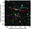 |
Fig. 1. Ground-based 140″ × 140″ DES g, r, y + z image of the galaxy cluster WHJ0400-27, with coordinates centred on the BCG (zcl, spec = 0.626, (RA, Dec)J2000 = (60.04888, −27.11959) deg). The cyan and red circles indicate the QSO pair (zspec = 1.345). The candidates for the third QSO image, with colours consistent with those of the QSOs, are enclosed by magenta squares (ID1-4-5-6). The dotted green rectangle represents the approximate region where the lens model predicts the position of the third image. Photometric cluster members are marked with orange circles. The dashed white line is the critical line predicted by the best-fit lens model at the QSO redshift. |
Properties of the multiple QSO images based on Gaia DR3.
By comparing our system with the list provided by Martinez et al. (2023, see their Table 3), we find that, if confirmed, QSO 0400-27 would rank as the fifth-largest-separation lensed QSO known to date. This ranking also takes into account the most recent QSO found by Napier et al. (2023).
3.2. Spectroscopic confirmation of the multiple QSO images
To confirm the nature of this double QSO system, we obtained the first long-slit spectra of QSO-A and QSO-B using the Alhambra Faint Object Spectrograph and Camera (ALFOSC, Djupvik & Andersen 2010), mounted at the 2.56 m Nordic Optical Telescope (NOT) at Roque de los Muchachos Observatory in La Palma, Spain, and the European Southern Observatory (ESO) Faint Object Spectrograph and Camera v2 (EFOSC2, Buzzoni et al. 1984), mounted at the 3.58 m New Technology Telescope (NTT) in Chile.
QSO-A and QSO-B were spectroscopically observed on November 15, 2023, with the ALFOSC/NOT instrument (programme ID 68-404, PI Bazzanini). The total integration time was 1 h (on-target), and a 1″-wide long slit was used, dispersed by grism #3 (covering a wavelength range of 3200–7070 Å), with a resolution of R ≃ 350 and a dispersion of 2.3 Å pixel−1. The average seeing was 0.6″ during the observation, with an average air mass of 2.1.
Both QSOs were also observed on February 12, 2024, using the EFOSC2/NTT (programme ID 112.25CT, PI Mannucci) to obtain a higher signal-to-noise ratio (S/N) and longer wavelength coverage. The total integration time was 45 min (on-target), and a 1″-wide long slit was used, dispersed by grism #4, covering a wavelength range between 4085 and 7520 Å, with a resolution of R ≃ 460, a dispersion of 1.68 Å pixel−1, an average seeing of 0.9″ during the observation, and an average air mass of 1.1.
We reduced all our data using the PypeIt data reduction pipeline (Prochaska et al. 2020), a Python package for the semi-automated reduction of astronomical spectroscopic data. We then flux-calibrated the NTT data using the standard star GD108 within the same pipeline. Due to the lack of spectroscopic standard observations with the adopted grism, we could not perform the flux calibration of the NOT spectra.
The reduced QSO spectra from the NOT and the NTT are shown at the top and bottom of Fig. 2, respectively. The S/N per pixel ranges from 5 to 8 (depending on wavelength) and is slightly higher in the NTT data. These observations suggest that the two QSO spectra are identical, with no measurable velocity shift. They have the same continuum shape, dust extinction, emission line shape, and line flux ratios. Indeed, a cross-correlation between the spectrum of each of the two QSOs and an SDSS QSO spectrum template extracted with the PANDORA Easy Z package (Garilli et al. 2010) yields the same redshift within δzNOT = 2 × 10⁻³, δzNTT = 3 × 10⁻⁴, resulting in  and confirming the values estimated in the Gaia catalogue. Moreover, the cross-correlation between the two observed QSO spectra (shown in the two insets in Fig. 2) peaks at ΔzNOT = (3 ± 8)×10−4 and at ΔzNTT = (3 ± 2)×10−4. The errors on the cross-correlation peak were estimated using a bootstrap procedure, which utilised 100 realisations of the QSO spectra by sampling the error spectrum from the data reduction pipeline. These values of Δz, which correspond to a rest-frame velocity difference of ≈40 km/s, are therefore fully consistent with zero. This implies no detectable velocity shift between the two spectra, supporting the SL nature of the event.
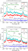 |
Fig. 2. Spectra of the two lensed QSO candidates (A and B, respectively in cyan and red) from NOT/ALFOSC (top) and NTT/EFOSC2 (bottom). The green curve is an SDSS QSO spectrum template. The vertical dotted lines (4475.97 Å, 5454.47 Å, and 6563.07 Å) represent the positions of emission lines of the corresponding ions redshifted to zQSO, spec = 1.345 of CIII] (1908.73 Å), CII] (2326 Å), and MgII (2798.75 Å), respectively. The two top-right insets show the cross-correlations of the QSO-A and QSO-B spectra. The bottom panel in each plot (blue line) shows the mean-subtracted relative flux difference of QSO-A with respect to QSO-B, the dashed red lines representing its rms. The grey bands highlight spectral regions with prominent sky emission lines, corresponding to significant residuals in the sky subtraction. |
The bottom panel of each plot in Fig. 2 shows the mean-subtracted relative flux difference of the two QSOs. This shows a rms of 7% and 9% for the NOT and NTT case, respectively, supporting the conclusion that the two QSOs have highly similar spectral properties. We note that differential flux calibration errors generally lead to longer-wavelength residuals, which is particularly evident in the NOT spectra.
The NOT spectra in Fig. 2a show some steepening on the blue side for QSO-A, while the NTT spectra do not. We can attribute this effect to differential atmospheric refraction (Filippenko 1982). We verified that it affects the NOT observations in a stronger fashion, due to the high air mass and the slit orientation being far from the parallactic angle. If the QSOs are not equally centred on the slit, this can lead to differential flux losses on the blue side of the spectra.
A close inspection of the NTT spectra in Fig. 2b also indicates that, assuming an optimal flux calibration across the entire wavelength range, the CIII and MgII emission peaks are of comparable strength for QSO-B, whereas for QSO-A they differ in strength by ≈15%. Should improved spectral observations confirm this discrepancy, it may, in the context of the SL scenario, result from differential levels of dust extinction and/or chromatic microlensing effects (e.g. Sluse et al. 2012).
An additional NOT spectrum, taken on December 2, 2023 (programme ID 68-404, PI Bazzanini), also confirmed the DES photometric redshift of the BCG, yielding zCL, spec = 0.626 (see Fig. 3). The total integration time was 1 h (on-target). Observations were performed using a 1.8″-wide long slit, dispersed by grism #7 (covering the wavelength range 3650–7110 Å). The spectral resolution was R ≃ 650, with a dispersion of 1.7 Å pixel−1, and the average seeing was 0.9″ during the observation.
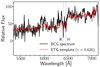 |
Fig. 3. NOT/ALFOSC 60 min (on-target) spectrum of the WHJ0400-27 BCG (black line). The red line is a redshifted early-type galaxy (ETG) spectrum template, which provides a significant cross-correlation peak at z = 0.626. The vertical dashed blue lines represent the positions of the redshifted CaII K and H absorption lines (3933.7 Å and 3968.5 Å). |
3.3. Strong lensing modelling
Assuming that the two QSOs are multiple images of the same background source, the SL model is inevitably poorly constrained, owing to the lack of additional multiple images and spectroscopic information of cluster member galaxies (with the exception of the BCG). The configuration of the double QSO suggests the existence of a third, less magnified, multiple image to the south of the BCG. To search for such an image, we built a preliminary SL model by using a single cluster-scale halo with an elliptical total mass distribution centred on the BCG. To this end, we used newly developed lens modelling software, Gravity.jl (Lombardi 2024), and independently validated the results with the public software lenstool (Kneib et al. 1996; Jullo et al. 2007; Jullo & Kneib 2009). For the cluster halo, we specifically adopted a non-singular isothermal ellipsoid with velocity dispersion, core radius, axis ratio, and position angle as free parameters; large flat priors were assumed on these parameters, and no priors were adopted on the position of the third image. The range of the flat priors on the free parameters used during the Monte Carlo Markov chain (MCMC) optimisation was:
-
Velocity dispersion: σ ∈ [100, 3000] km/s;
-
Core radius: s ∈ [10−4, 50] arcsec;
-
Axis-ratio: q ∈ [0.5, 1];
-
Position angle (clockwise from north): θ ∈ [ − π/2, π/2].
We used a 0.1″ positional uncertainty for QSO-A and QSO-B.
The model optimisation yielded the following formal values for the median and the 1σ errors:  km/s,
km/s,  arcsec, and
  ,
,  . The optimised model predicts a magnitude difference ΔGAB ≈ 0 between QSO-A and QSO-B, whereas the observed Gaia value is ΔGAB ≈ 0.4. We note that by using the QSOs’ flux ratio as an additional model constraint, mass models with high ellipticities are preferred in the optimisation. In Fig. 1 we include a dotted green rectangle representing the approximate region where the third image is predicted by the lens model, based on the positional distribution of 5000 MCMC samples of the posterior parameters.
We also carried out an independent search for third image candidates by selecting point-like sources with colours consistent with those of QSO-A and QSO-B in the four-dimensional colour space (g − r, r − i, i − z, and z − y). This search was performed using the DES DR2 five-band photometric catalogue (Abbott et al. 2021) and led us to identify four possible candidates (see the magenta squares in Fig. 1). One of these, ID5, has the smallest rms colour difference in the four-dimensional colour space (Δm = 0.08 ± 0.06) with respect to the QSOs, and appears unresolved under the 1.2″ seeing conditions. If the third image were confirmed through follow-up spectroscopic observations within the predicted region shown in Fig. 1, QSO 0400-27 would qualify as one of the largest-separation strongly lensed QSOs ever observed.
However, two critical aspects emerge from the predictions based on this poorly constrained (i.e., four free parameters but two constraints) model: i) The third image is predicted to be 1.1 ± 0.3 mag fainter than QSO-A. In contrast, ID5, with gDES ≃ 22.6, appears to be ≈2.4 mag fainter (gDES, QSO − A ≃ 20.2), making it a less convincing candidate. ii) The lens model predicts an encircled cluster mass within 30″ (≈205 kpc at z = 0.63) of (3 ± 1) × 1014 M⊙. This would make it particularly massive compared to the DES richness parameter (Wen & Han 2024) and, more importantly, to the independent limits inferred from X-ray and Sunyaev–Zeldovich (SZ) surveys. We discuss this point further in the next section.
4. Discussion
Even though the strong similarities between the two QSO spectra suggest that this system is two multiple images of the same background QSO, lying behind a relatively rich galaxy cluster at z = 0.626 (see the BCG spectrum in Fig. 3), we also considered the possibility that the QSO 0400-27 system is a projected physical association of two QSOs. In the simplified case where the deflection contribution of the intervening lens cluster is entirely neglected, the observed two-dimensional separation of approximately 18″ would correspond to a maximum projected physical distance of ≈150 kpc, at z = 1.345, for two distinct QSOs. Several studies have focused on the search for dual AGNs over a wide range of physical separations, from kiloparsec scales (Chen et al. 2022; Mannucci et al. 2023) to > 10 kpc and up to 150 kpc (Hennawi et al. 2006; Liu et al. 2011; Eftekharzadeh et al. 2017). A number of dual QSOs with velocity differences (< 100 km/s) and separations (∼100–150 kpc) similar to those in our system have been identified. However, their spectra show noticeable differences, contrary to what we observe. The system with the most similar characteristics to QSO 0400-27 is SDSS J1010+0416 (Hennawi et al. 2006), which consists of two QSOs at z = 1.52 separated by ≈150 kpc. The rest frame velocity difference of SDSS J1010+0416 based on the MgII emission line is ≈40 km/s, even though the two MgII lines appear to have different widths. In contrast, the CIII lines show a velocity offset of ≈2000 km/s. For QSO 0400-27 we detect no shifts in both the CIII and MgII lines (Δvrest ≲ 40 km/s).
As mentioned above, there is a noticeable tension when comparing the encircled lensing mass to M500 estimated from optical mass proxies. This comparison, however, is affected by significant systematic errors arising from the uncertain extrapolation of the SL mass to much larger radii as well as from uncertainties in the cluster mass calibration based on richness parameters. In this respect, a more meaningful test would be to check whether X-ray emission is expected in the extended ROentgen Survey with an Imaging Telescope Array (eROSITA) survey data (Predehl et al. 2021) based on the estimated lensing mass of WHJ0400-27. To this end, we inspected the eROSITA All-Sky Survey (eRASS) catalogue of 12 247 clusters published in Bulbul et al. (2024). Neither our system nor the two QSOs are detected, which would be blended in the eROSITA point spread function. By estimating a lower limit for the X-ray luminosity (LX [0.2−2.3 keV] ≈ 1044 erg s−1, within their adopted R500) in the vicinity of WHJ0400-27 – using the flux limit in that survey region and the cluster redshift – we find that a cluster with a mass in excess of M500 ≈ 5 × 10¹⁴ M⊙ should be detected in the eRASS data. This seems to be in tension with the SL mass extrapolated to R500, which we estimate as M500 ≈ 8 × 10¹⁴ M⊙ using the best-fit mass-density profile from our lens model. However, these estimates are affected by significant systematic uncertainties.
As a further point of consideration, we note that our cluster is not detected in the Atacama Cosmology Telescope (ACT) SZ survey from the DR5 Multi-Component Matched Filter (MCMF) cluster catalogue (Klein et al. 2024), where several clusters at similar redshifts have been identified with masses down to M500 ≈ 2 × 10¹⁴ M⊙. Both the X-ray- and SZ-based mass lower limits seem to indicate a tension with the lens-model-based mass, which, at face value, is a factor of ≈2 − 4, notwithstanding all the uncertainties in the quoted mass values.
5. Conclusion
As part of a search for Gaia QSOs gravitationally lensed by galaxy clusters, we present the discovery of a pair of QSOs separated by Δϑ = 17.8″ at zQSO, spec = 1.345 with remarkable spectral similarities lying in the projected vicinity of the galaxy cluster candidate WHJ0400-27 at zCL, phot = 0.63. Our two independent spectroscopic studies, carried out with the ESO/NTT and NOT telescopes, show indistinguishable spectra for the two QSOs. There is no measurable redshift difference (below the third decimal digit), and the continuum, emission line shapes, and line flux ratios are all very similar (see Fig. 2).
We first investigated the SL scenario by building a model of the optically selected cluster using a single-component mass distribution centred on the BCG (zBCG, spec = 0.626). We used the position of the two QSOs – located at projected distances of 31.5″ and 24.5″ from the BCG – as the only model constraint. This model predicts the existence of a third lensed image, which remains to be found among a number of candidates selected from sources with similar morphologies and colours. Notably, our poorly constrained lensing model predicts a cluster mass that appears to be higher (by a factor 2–4) than mass upper limits obtained from the lack of X-ray and SZ detections in the eROSITA and ACT surveys, respectively. Even though systematic uncertainties remain large when comparing the SL mass of WHJ0400-27 to that inferred from other mass proxies (richness, X-rays, and SZ), this raises questions about the lensing nature of the QSO pair. Interestingly, studies of several other SL systems on galaxy scales face similar challenges (e.g. Anguita et al. 2018; Lemon et al. 2022). It is therefore worth exploring the possibility that QSO 0400-27 represents a physical association of two QSOs, separated by approximately 150 kpc in projection behind WHJ0400-27, but outside the SL regime. While dual AGNs with such large separations and small velocity shifts are rare, the few observed have been found with noticeable differences in their spectra (e.g. line widths; see Hennawi et al. 2006). We therefore conclude that the combination of physical separation and nearly identical spectra would make our dual QSO system rather unique.
Planned follow-up spectroscopic and imaging observations will be crucial to significantly improving the modelling constraints of the lens cluster, specifically by identifying the predicted third image and by confirming a sizable number of cluster galaxies. Should we be able to confirm the gravitational lensing nature of our system, QSO 0400-27 has the potential to become the largest-separation lensed QSO known to date, holding great promise for TDC applications.
Acknowledgments
We thank the anonymous referee for the helpful and insightful comments that improved the paper. LB is indebted to the communities behind the multiple free, libre, and open-source software packages on which we all depend on. PR conceived the research; LB, GA, and PR developed the methodology; LB, GA, MS, PB and GDR performed all the numerical work, including software development, investigation, and validation. All authors contributed to the discussion of the results, the editing and revision of the paper. We acknowledge support from the Italian Ministry of University and Research through grant PRIN-MIUR 2020SKSTHZ. This publication was produced while attending the PhD program in PhD in Space Science and Technology at the University of Trento, Cycle XXXIX, with the support of a scholarship financed by the Ministerial Decree no. 118 of 2nd march 2023, based on the NRRP – funded by the European Union – NextGenerationEU – Mission 4 “Education and Research”, Component 1 “Enhancement of the offer of educational services: from nurseries to universities” – Investment 4.1 “Extension of the number of research doctorates and innovative doctorates for public administration and cultural heritage”. Based on observations made with the Nordic Optical Telescope, owned in collaboration by the University of Turku and Aarhus University, and operated jointly by Aarhus University, the University of Turku and the University of Oslo, representing Denmark, Finland and Norway, the University of Iceland and Stockholm University at the Observatorio del Roque de los Muchachos, La Palma, Spain, of the Instituto de Astrofisica de Canarias. The data presented here were obtained [in part] with ALFOSC, which is provided by the Instituto de Astrofisica de Andalucia (IAA) under a joint agreement with the University of Copenhagen and NOT. Based on observations collected at the European Organisation for Astronomical Research in the Southern Hemisphere under ESO programme 112.25CT. This work uses the following software packages: Python (Van Rossum & Drake 2009), NumPy (van der Walt et al. 2011; Harris et al. 2020), SciPy (Virtanen et al. 2020), Astropy (Astropy Collaboration 2013; Price-Whelan et al. 2018), matplotlib (Hunter 2007), PypeIt (Prochaska et al. 2020), (Lombardi 2024), Lenstool (Kneib et al. 1996; Jullo et al. 2007; Jullo & Kneib 2009), WebPlotDigitizer (Rohatgi 2024) (Rohatgi 2024), ds9 (Joye et al. 2003), Aladin (Bonnarel et al. 2000), topcat (Taylor 2005), bash (Gnu 2007).
References
- Abbott, T. M. C., Adamów, M., Aguena, M., et al. 2021, ApJS, 255, 20 [NASA ADS] [CrossRef] [Google Scholar]
- Anguita, T., Schechter, P. L., Kuropatkin, N., et al. 2018, MNRAS, 480, 5017 [NASA ADS] [Google Scholar]
- Astropy Collaboration (Robitaille, T. P., et al.) 2013, A&A, 558, A33 [NASA ADS] [CrossRef] [EDP Sciences] [Google Scholar]
- Birrer, S., Amara, A., & Refregier, A. 2016, JCAP, 2016, 020 [CrossRef] [Google Scholar]
- Bonnarel, F., Fernique, P., Bienaymé, O., et al. 2000, A&AS, 143, 33 [NASA ADS] [CrossRef] [EDP Sciences] [Google Scholar]
- Bulbul, E., Liu, A., Kluge, M., et al. 2024, A&A, 685, A106 [NASA ADS] [CrossRef] [EDP Sciences] [Google Scholar]
- Buzzoni, B., Delabre, B., Dekker, H., et al. 1984, The Messenger, 38, 9 [NASA ADS] [Google Scholar]
- Chen, Y.-C., Hwang, H.-C., Shen, Y., et al. 2022, ApJ, 925, 162 [NASA ADS] [CrossRef] [Google Scholar]
- Dahle, H., Gladders, M. D., Sharon, K., et al. 2013, ApJ, 773, 146 [NASA ADS] [CrossRef] [Google Scholar]
- Dark Energy Survey Collaboration (Abbott, T., et al.) 2016, MNRAS, 460, 1270 [Google Scholar]
- Djupvik, A. A., & Andersen, J. 2010, in Highlights of Spanish Astrophysics V, Astrophys. Space Sci. Proc., 14, 211 [NASA ADS] [CrossRef] [Google Scholar]
- Dutta, R., Acebron, A., Fumagalli, M., et al. 2024, MNRAS, 528, 1895 [CrossRef] [Google Scholar]
- Eftekharzadeh, S., Myers, A. D., Hennawi, J. F., et al. 2017, MNRAS, 468, 77 [NASA ADS] [CrossRef] [Google Scholar]
- Euclid Collaboration (Adam, R., et al.) 2019, A&A, 627, A23 [NASA ADS] [CrossRef] [EDP Sciences] [Google Scholar]
- Filippenko, A. V. 1982, PASP, 94, 715 [Google Scholar]
- Gaia Collaboration (Bailer-Jones, C. A. L., et al.) 2023, A&A, 674, A41 [NASA ADS] [CrossRef] [EDP Sciences] [Google Scholar]
- Garilli, B., Fumana, M., Franzetti, P., et al. 2010, PASP, 122, 827 [Google Scholar]
- Gnu, P. 2007, Free Software Foundation. Bash (3.2. 48)[Unix shell program] [Google Scholar]
- Grillo, C., Rosati, P., Suyu, S. H., et al. 2018, ApJ, 860, 94 [Google Scholar]
- Grillo, C., Rosati, P., Suyu, S. H., et al. 2020, ApJ, 898, 87 [Google Scholar]
- Grillo, C., Pagano, L., Rosati, P., & Suyu, S. H. 2024, A&A, 684, L23 [NASA ADS] [CrossRef] [EDP Sciences] [Google Scholar]
- Harris, C. R., Millman, K. J., van der Walt, S. J., et al. 2020, Nature, 585, 357 [NASA ADS] [CrossRef] [Google Scholar]
- Hennawi, J. F., Strauss, M. A., Oguri, M., et al. 2006, AJ, 131, 1 [Google Scholar]
- Hunter, J. D. 2007, Comput. Sci. Eng., 9, 90 [NASA ADS] [CrossRef] [Google Scholar]
- Inada, N., Oguri, M., Pindor, B., et al. 2003, Nature, 426, 810 [NASA ADS] [CrossRef] [Google Scholar]
- Inada, N., Oguri, M., Morokuma, T., et al. 2006, ApJ, 653, L97 [Google Scholar]
- Ivezić, Ž., Kahn, S. M., Tyson, J. A., et al. 2019, ApJ, 873, 111 [Google Scholar]
- Joye, W. A., & Mandel, E. 2003, in Astronomical Data Analysis Software and Systems XII, eds. H. E. Payne, R. I. Jedrzejewski, & R. N. Hook, ASP Conf. Ser., 295, 489 [NASA ADS] [Google Scholar]
- Jullo, E., & Kneib, J. P. 2009, MNRAS, 395, 1319 [NASA ADS] [CrossRef] [Google Scholar]
- Jullo, E., Kneib, J. P., Limousin, M., et al. 2007, New J. Phys., 9, 447 [Google Scholar]
- Kelly, P. L., Rodney, S. A., Treu, T., et al. 2015, Science, 347, 1123 [Google Scholar]
- Klein, M., Mohr, J. J., Bocquet, S., et al. 2024, MNRAS, 531, 3973 [NASA ADS] [CrossRef] [Google Scholar]
- Kneib, J. P., Ellis, R. S., Smail, I., Couch, W. J., & Sharples, R. M. 1996, ApJ, 471, 643 [Google Scholar]
- Lang, D. 2014, AJ, 147, 108 [Google Scholar]
- Lemon, C., Millon, M., Sluse, D., et al. 2022, A&A, 657, A113 [NASA ADS] [CrossRef] [EDP Sciences] [Google Scholar]
- Liu, X., Shen, Y., Strauss, M. A., & Hao, L. 2011, ApJ, 737, 101 [Google Scholar]
- Lombardi, M. 2024, A&A, 690, A346 [NASA ADS] [CrossRef] [EDP Sciences] [Google Scholar]
- Mannucci, F., Scialpi, M., Ciurlo, A., et al. 2023, A&A, 680, A53 [NASA ADS] [CrossRef] [EDP Sciences] [Google Scholar]
- Martinez, M. N., Napier, K. A., Cloonan, A. P., et al. 2023, ApJ, 946, 63 [NASA ADS] [CrossRef] [Google Scholar]
- Moresco, M., Amati, L., Amendola, L., et al. 2022, Liv. Rev. Relat., 25, 6 [NASA ADS] [Google Scholar]
- Napier, K., Gladders, M. D., Sharon, K., et al. 2023, ApJ, 954, L38 [NASA ADS] [CrossRef] [Google Scholar]
- Predehl, P., Andritschke, R., Arefiev, V., et al. 2021, A&A, 647, A1 [EDP Sciences] [Google Scholar]
- Price-Whelan, A. M., Sipőcz, B. M., Günther, H. M., et al. 2018, AJ, 156, 123 [NASA ADS] [CrossRef] [Google Scholar]
- Prochaska, J., Hennawi, J., Westfall, K., et al. 2020, J. Open Source Software, 5, 2308 [NASA ADS] [CrossRef] [Google Scholar]
- Refsdal, S. 1964, MNRAS, 128, 307 [NASA ADS] [CrossRef] [Google Scholar]
- Rohatgi, A. 2024, WebPlotDigitizer, https://automeris.io/WebPlotDigitizer.html [Google Scholar]
- Schlafly, E. F., Meisner, A. M., & Green, G. M. 2019, ApJS, 240, 30 [Google Scholar]
- Shu, Y., Marques-Chaves, R., Evans, N. W., & Pérez-Fournon, I. 2018, MNRAS, 481, L136 [Google Scholar]
- Shu, Y., Koposov, S. E., Evans, N. W., et al. 2019, MNRAS, 489, 4741 [Google Scholar]
- Sluse, D., Hutsemékers, D., Courbin, F., Meylan, G., & Wambsganss, J. 2012, A&A, 544, A62 [NASA ADS] [CrossRef] [EDP Sciences] [Google Scholar]
- Suyu, S. H., Bonvin, V., Courbin, F., et al. 2017, MNRAS, 468, 2590 [Google Scholar]
- Taylor, M. B. 2005, in Astronomical Data Analysis Software and Systems XIV, eds. P. Shopbell, M. Britton, & R. Ebert, ASP Conf. Ser., 347, 29 [Google Scholar]
- Treu, T., Suyu, S. H., & Marshall, P. J. 2022, A&A Rev., 30, 8 [NASA ADS] [CrossRef] [Google Scholar]
- van der Walt, S., Colbert, S. C., & Varoquaux, G. 2011, Comput. Sci. Eng., 13, 22 [Google Scholar]
- Van Rossum, G., & Drake, F. L. 2009, Python 3 Reference Manual (Scotts Valley, CA: CreateSpace) [Google Scholar]
- Verde, L., Treu, T., & Riess, A. G. 2019, Nat. Astron., 3, 891 [Google Scholar]
- Virtanen, P., Gommers, R., Oliphant, T. E., et al. 2020, Nat. Methods, 17, 261 [Google Scholar]
- Wen, Z. L., & Han, J. L. 2022, MNRAS, 513, 3946 [NASA ADS] [CrossRef] [Google Scholar]
- Wen, Z. L., & Han, J. L. 2024, ApJS, 272, 39 [NASA ADS] [CrossRef] [Google Scholar]
- Wong, K. C., Suyu, S. H., Chen, G. C. F., et al. 2020, MNRAS, 498, 1420 [Google Scholar]
- Wright, E. L., Eisenhardt, P. R. M., Mainzer, A. K., et al. 2010, AJ, 140, 1868 [Google Scholar]
All Tables
All Figures
|
Fig. 1. Ground-based 140″ × 140″ DES g, r, y + z image of the galaxy cluster WHJ0400-27, with coordinates centred on the BCG (zcl, spec = 0.626, (RA, Dec)J2000 = (60.04888, −27.11959) deg). The cyan and red circles indicate the QSO pair (zspec = 1.345). The candidates for the third QSO image, with colours consistent with those of the QSOs, are enclosed by magenta squares (ID1-4-5-6). The dotted green rectangle represents the approximate region where the lens model predicts the position of the third image. Photometric cluster members are marked with orange circles. The dashed white line is the critical line predicted by the best-fit lens model at the QSO redshift. |
| In the text | |
|
Fig. 2. Spectra of the two lensed QSO candidates (A and B, respectively in cyan and red) from NOT/ALFOSC (top) and NTT/EFOSC2 (bottom). The green curve is an SDSS QSO spectrum template. The vertical dotted lines (4475.97 Å, 5454.47 Å, and 6563.07 Å) represent the positions of emission lines of the corresponding ions redshifted to zQSO, spec = 1.345 of CIII] (1908.73 Å), CII] (2326 Å), and MgII (2798.75 Å), respectively. The two top-right insets show the cross-correlations of the QSO-A and QSO-B spectra. The bottom panel in each plot (blue line) shows the mean-subtracted relative flux difference of QSO-A with respect to QSO-B, the dashed red lines representing its rms. The grey bands highlight spectral regions with prominent sky emission lines, corresponding to significant residuals in the sky subtraction. |
| In the text | |
|
Fig. 3. NOT/ALFOSC 60 min (on-target) spectrum of the WHJ0400-27 BCG (black line). The red line is a redshifted early-type galaxy (ETG) spectrum template, which provides a significant cross-correlation peak at z = 0.626. The vertical dashed blue lines represent the positions of the redshifted CaII K and H absorption lines (3933.7 Å and 3968.5 Å). |
| In the text | |
Current usage metrics show cumulative count of Article Views (full-text article views including HTML views, PDF and ePub downloads, according to the available data) and Abstracts Views on Vision4Press platform.
Data correspond to usage on the plateform after 2015. The current usage metrics is available 48-96 hours after online publication and is updated daily on week days.
Initial download of the metrics may take a while.