| Issue |
A&A
Volume 698, June 2025
|
|
|---|---|---|
| Article Number | A128 | |
| Number of page(s) | 10 | |
| Section | Cosmology (including clusters of galaxies) | |
| DOI | https://doi.org/10.1051/0004-6361/202450840 | |
| Published online | 06 June 2025 | |
Investigating the impact of galaxies’ compact binary hosting probability for gravitational wave cosmology
1
Dipartimento di Fisica e Astronomia “Galileo Galilei”, Università degli Studi di Padova, Via Marzolo 8, I-35131 Padova, Italy
2
INFN, Sezione di Padova, Via Marzolo 8, I-35131 Padova, Italy
3
INFN, Sezione di Roma, I-00185 Roma, Italy
4
Dipartimento di Fisica “Enrico Fermi”, Università di Pisa, Largo Bruno Pontecorvo 3, Pisa I-56127, Italy
5
INFN, Sezione di Pisa, Largo Bruno Pontecorvo 3, Pisa I-56127, Italy
⋆ Corresponding author: This email address is being protected from spambots. You need JavaScript enabled to view it.
Received:
23
May
2024
Accepted:
9
April
2025
Abstract
With the advent of future-generation interferometers, a huge number of gravitational wave (GW) signals without electromagnetic counterparts are expected to be measured. Although these signals do not allow a simultaneous measurement of the redshift and the luminosity distance, it is still possible to infer cosmological parameters. In this paper we focus on the systematic biases that could arise from mismodelling the GW host probability when inferring the Hubble constant (H0) using GW dark sirens jointly with galaxy catalogues. We discuss the case in which the GW host probability is a function of galaxy luminosity and redshift, as it has been predicted by synthetic state-of-the-art compact binary coalescence catalogues. We show that, in the limiting case in which the analysis is done with a complete galaxy catalogue covering a footprint of ∼10 deg2, mismatching the host probability in terms of galaxy’s luminosity will introduce a bias on H0. In this case, the magnitude of the bias will depend on the distribution of the large-scale structure over the line of sight. Instead, in the limit of a complete wide-field-of-view galaxy catalogue and GW events localized at the 𝒪(Gpc) distance, mismatching the redshift dependence of the GW hosting probability is more likely to introduce a systematic bias.
Key words: cosmological parameters / cosmology: theory
© The Authors 2025
 Open Access article, published by EDP Sciences, under the terms of the Creative Commons Attribution License (https://creativecommons.org/licenses/by/4.0), which permits unrestricted use, distribution, and reproduction in any medium, provided the original work is properly cited.
This article is published in open access under the Subscribe to Open model. This email address is being protected from spambots. You need JavaScript enabled to view it. to support open access publication.
1. Introduction
The first observation of a gravitational wave (GW) signal in 2015 (Abbott et al. 2016) opened a new complementary way to access information about our Universe, on both the astrophysical and cosmological sides. On the astrophysical side, after the detection of a further 90 GW events, it has become feasible to infer not only information about the individual sources emitting GWs but also about the mass and spin distributions of the entire population of compact binaries (Abbott et al. 2023a, 2021a). On the cosmological side, GWs can be used to probe the cosmic expansion (Schutz 1986; Holz & Hughes 2005; Dalal et al. 2006) independently of other probes, such as Supernovae (Galbany et al. 2023) and the Cosmic Microwave Background (Planck Collaboration VI 2020). This is possible thanks to the fact that GWs directly provide a measurement of the source luminosity distance. Therefore, if provided with a source redshift estimation, GW sources can be used to probe the cosmic expansion. Unfortunately, GWs alone cannot provide a direct measurement of the redshift since it is degenerate with the source masses. A direct estimation of the redshift can be obtained if an electromagnetic counterpart (EM) to the GW source is observed. The EM counterpart could allow the identification of the host galaxy, for which it is typically possible to measure the redshift with spectroscopic observations. This was the case for the binary neutron star merger GW170817 (Abbott et al. 2017a,b), for which it was possible to estimate  km/s/Mpc at a 68.3% credible interval (C. I.). Since then, no additional GW event has been observed with an EM counterpart.
As first argued by Schutz (1986), even in the absence of an EM, GW sources can still be employed to measure the cosmic expansion (dark sirens method). There are several techniques proposed in the literature to use dark sirens for cosmology, such as the source-frame mass method (Chernoff & Finn 1993; Taylor et al. 2012; Farr 2019; Ezquiaga & Holz 2021; Mastrogiovanni et al. 2021; Mukherjee 2022; Leyde et al. 2022; Ezquiaga & Holz 2022; Karathanasis et al. 2023) and cross-correlations with large-scale structure tracers (Oguri 2016); Mukherjee:2019wcg; Mukherjee:2020hyn; Bera:2020jhx. In this work we focus on the ‘galaxy catalogue’ technique first proposed by Schutz (1986). This technique consists of assigning a statistical redshift measurement by using the GW source localization and all the galaxies reported in a given survey (Del Pozzo 2012; Chen et al. 2018; Gray et al. 2020, 2022; Leandro et al. 2022; Gair et al. 2023). This is possible since every astrophysical GW event is expected to be hosted in a galaxy1. Although the galaxy catalogue method is less precise when inferring H0 than a single event with an EM counterpart, it is expected to play a relevant role for GW cosmology given the number of dark siren detections, as demonstrated by its current applications (Fishbach et al. 2019; Soares-Santos et al. 2019; Abbott et al. 2021b, 2023b; Palmese et al. 2020, 2023; Finke et al. 2021; Mastrogiovanni et al. 2023; Borghi et al. 2024). Furthermore, with the advent of future-generation interferometers such as LISA (Auclair et al. 2023), Cosmic Explorer (CE; Evans et al. 2021), and Einstein Telescope (ET; Maggiore et al. 2020; Branchesi 2023), a much higher number of GW signals are expected to be detected, further emphasizing the importance of such an analysis.
A central topic of the galaxy catalogue method is how to describe for each galaxy the probability that it hosts a GW event. The simplest choice might be to assume that every galaxy has an equal probability of hosting a GW event; however, this is not a physically motivated assumption as we observe that the overall star formation rate (SFR), and hence the compact objects produced, correlates with several galactic properties (Madau & Dickinson 2014). Furthermore, as shown in Hanselman et al. (2025), assuming equal host probabilities can lead to biases in the estimated value of H0. As such, current analyses include a hosting probability based on the intrinsic luminosity of the galaxies, namely the brighter the galaxy, the more likely it is to host a GW event (some recent predictions for host galaxy properties are discussed in Vijaykumar et al. 2024 and Artale et al. 2020). Gray et al. (2020) show that luminosity weights can boost the H0 precision; however, no study has been conducted on the systematics on H0 that these assumptions can introduce.
In this work we studied in detail how modelling the GW host probability can introduce systematics when inferring H0. We based our study on the simulation approach presented in Gair et al. (2023). Starting from a simulated Universe (MICEcat; Crocce et al. 2015), we populated GW events in each galaxy following a hosting probability model obtained from synthetic catalogues of compact binary coalescences (CBCs; Artale et al. 2020). We then used different selection criteria for the GW events and different GW hosting probability models to study possible biases for the H0 inference.
We start in Sect. 2 by describing the statistical framework we considered in our analysis. In Sect. 3 we present the simulated Universe considered for the simulation and our GW data generation technique. Finally, in Sect. 4 we discuss the results of our analysis, while in Sect. 5 we report our conclusions.
2. Statistical framework
2.1. General prescription for H0 inference
The posterior on H0 inferred from the detection of NGW events from a collection of data {x}, can be obtained using the Bayes theorem (e.g. Sivia & Skilling 2006),
 (1)
(1)
where p(H0) is a prior and ℒ({x}|H0) the likelihood. The likelihood describes the GW detection as an inhomogeneous Poisson process in the presence of selection biases (Mandel et al. 2019; Vitale et al. 2020). Neglecting the information on the binary masses, for the galaxy catalogue technique the likelihood can be written as (Gair et al. 2023)
![Mathematical equation: $$ \begin{aligned} \mathcal{L} (\{x\}|H_0)&\propto e^{-N_{\rm exp}(H_0)}[N_{\rm exp}(H_0)]^{N_{\rm GW}} \nonumber \\&\quad \times \prod _i^{N_{\rm GW}} \frac{\int dz d\Omega \mathcal{L} _{\rm GW}(x_i|d_{\rm L}(z,H_0),\Omega )p_{\rm CBC}(z,\Omega )}{\int dz d\Omega P_{\rm det}^\mathrm{GW}(z, H_0,\Omega )p_{\rm CBC}(z,\Omega )}, \end{aligned} $$](/articles/aa/full_html/2025/06/aa50840-24/aa50840-24-eq3.gif) (2)
(2)
where Nexp is the expected number of GW detections, z the source redshift, Ω the sky location, ℒGW(xi|dL(z, H0),Ω) the GW likelihood (i.e. how well we can measure the luminosity distance and sky position),  the GW detection probability and pCBC(z, Ω) the probability of finding CBC at redshift z and sky position Ω. By assuming that the GW likelihood is reasonably constant in a given sky area, Ωloc, and that the detection probability does not vary in this sky area (i.e.
  , Eq. (2) can be rewritten dropping the sky-localization dependence and defining pCBC, loc(z)∝pCBC(z, Ωloc). In the remainder of the paper we refer to pCBC, loc(z) as simply pCBC(z) for brevity. Later in this section we explain how to construct pCBC(z) taking into account a non-trivial GW hosting probability. Equation (2) can be marginalized analytically on Nexp (Fishbach et al. 2018) by assuming a flat-in-log prior and thus obtaining the identity
 (3)
(3)
For this work, we modelled the GW likelihood using the toy model from Gair et al. (2023),
 (4)
(4)
where we identify the data chunk xi as an ‘observed’ luminosity distance,  , to which we applied a selection cut. In Eq. above, A = 0.2 is chosen to mimic a typical error budget on the luminosity distance of 20%. As argued in Gair et al. (2023), it is important to apply the selection cut strictly on the observed luminosity distance to avoid introducing a systematic bias due to the incongruent statistical model (see Essick & Fishbach 2024 for a detailed discussion on physical and unphysical statistical models). The detection probability is defined for each ‘true’ dL by integrating over all the observable datasets,
  . Following Gair et al. (2023), we assumed that GWs are detected if their observed luminosity distance is lower than a certain horizon,
  , namely
![Mathematical equation: $$ \begin{aligned} P_{\rm det}^\mathrm{GW} (d_L)&= \int _{-\infty }^{\hat{d}_L^\mathrm{thr}} \mathcal{L} _{\rm GW} (\hat{d}_L|d_L(z,H_0)) d\hat{d}_L \nonumber \\&= \frac{1}{2} \left[1 + \mathrm{{erf}}\left(\frac{d_L(z,H_0)-\hat{d}_L^\mathrm{thr}}{\sqrt{2}A d_L(z,H_0)}\right)\right]. \end{aligned} $$](/articles/aa/full_html/2025/06/aa50840-24/aa50840-24-eq11.gif) (5)
(5)
This simple prescription of the GW detection horizon is nearly equivalent to considering a selection criteria based on the signal-to-noise ratio (SNR). In fact, for GW sources, the SNR is proportional to the inverse of the luminosity distance. Before proceeding to the construction of a galaxy-informed pCBC(z), let us clarify that this type of statistical framework does not apply to real data. In a realistic scenario, the GW detection probability will depend on other parameters such as the detector masses of the GW signals. Moreover, we are not able to define a model that approximates xi with ‘observed’ quantities. As such, real data analysis techniques, such as that used in Mastrogiovanni et al. (2024), employ parameter estimation samples generated from data xi in synergy with an injection campaign to correct selection biases. For all these reasons, the computational complexity does not allow for an extensive and straightforward Monte Carlo study on how the GW hosting probability translates to a H0 bias.
2.2. Building the compact binary coalescence probability
We modelled pCBC(z) following Mastrogiovanni et al. (2023), Gray et al. (2023), and Borghi et al. (2024):
 (6)
(6)
where frate is a function that parametrizes the probability that a galaxy with redshift z and absolute magnitude M hosts a GW signal, while pcat(z, M) is the distribution of galaxies in terms of redshift and absolute magnitude in a given sky pixel2. This parametrization of pCBC(z) is an extension to the one provided in Gair et al. (2023) that considered only a dependence of the CBC rate from the galaxy redshift. Moreover, this parameterization requires that the redshift and apparent magnitude (from which the absolute magnitude is computed) be accurately measured; otherwise, a prior term on the distribution of absolute magnitudes in the Universe should be included. In principle, we could extend Eq. (6) to include any galactic property. Here we just focus on the absolute magnitude (i.e. intrinsic luminosity) as it is the galactic property typically used to model the GW hosting probability. Before describing the modellization of frate(z, M), let us briefly comment on Eq. (6). If all the galaxies are equally likely to host a GW source, then frate(z, M) is constant and
 (7)
(7)
In other words, the distribution of possible CBC hosts will coincide to the distribution of galaxies over the line of sight (LOS). However, if frate(z, M) is not uniform, this will not be the case.
We modelled the rate function using a model similar to that employed by Mastrogiovanni et al. (2023), namely
 (8)
(8)
where M* is the Schechter function knee value for the galaxies’ luminosity distribution. ψCBC(z) is a function that we computed numerically to parameterize the CBC merger rate as a function of redshift (see Sect. 3) and
 (9)
(9)
a term that introduces a power-law dependence for the host probability, which depends on the galaxies’ intrinsic luminosity. This simple parametrization is inspired by Artale et al. (2020), who argue, based on synthetic simulations of CBCs, that the CBC merger rate has a dependence on the galaxies’ redshift (due to the different SFRs and time delays) and the galaxies’ luminosity (due to the total stellar mass).
Finally, let us discuss how we calculated and employed pcat(z, M) in practice. Assuming that we are provided with a complete galaxy catalogue reporting Ngal galaxies with a collection of redshifts  and apparent magnitudes
  , then following Gair et al. (2023) and Mastrogiovanni et al. (2023) we have
 (10)
(10)
where the terms indicated with p(⋅) are the single posteriors on each galaxy true redshift and apparent magnitude. To better focus on the systematics introduced by the modelling of frate(z, M), we assumed that we have perfectly measured redshift and apparent magnitude of the galaxies. These are reasonable assumptions for galaxies whose redshift is estimated with spectroscopic observations. When the errors on the galaxies’ redshift and apparent magnitude are small,
 (11)
(11)
In practice, we never compute pcat(z, M). In fact by substituting Eq. (11) into Eq. (6) and later considering the hierarchical likelihood in Eq. (3), with the GW likelihood model in Eq. (4), it is possible to show that
 (12)
(12)
3. Simulation setup and catalogue description
We provide an overview of the data products and simulation procedures used for this study. In Sect. 3.1 we describe the MICEcat catalogue, a simulated Universe used to assign the GW galaxy hosts. In Sect. 3.2 we discuss the procedure to generate the GW signals starting from the galaxies list and in Sect. 3.3 we discuss some of the features of the GW catalogues generated from the simulation.
3.1. Description of MICEcat and the GW host probability model
We used MICEcat, a galaxy catalogue generated from the MICE Grand Challenge light-cone simulation (Fosalba et al. 2015a,b; Crocce et al. 2015; Carretero et al. 2015; Hoffmann et al. 2015); it is a full N-body simulation of the Universe containing about 70 billion dark matter particles. MICEcat has been generated using the following set of cosmological parameters, Ωm = 0.25, σ8 = 0.8, ns = 0.95, Ωb = 0.044, ΩΛ = 0.75, h = 0.7 for a fiducial ΛCDM model. The light-cone simulation has been performed in the redshift range 0 < z < 1.4, and using a hybrid halo occupation distribution and halo abundance matching prescriptions to populate friends-of friends dark matter halos, whose masses are greater than 2.2 ⋅ 1011 M⊙/h (Crocce et al. 2015). MICEcat reports the true redshift and the true absolute magnitude Mr in the infrared band (r band) for all the galaxies. The catalogue covers only 1/8 of the full sky in the redshift range and is complete up to redshift 1.4.
We modelled the GW host probability for each event using the parametrization for frate in Eq. (8). The redshift dependence of the CBC rate function was obtained with the procedure used in Bellomo et al. (2022). We started from the phenomenological expression provided for the SFR in Madau & Dickinson (2014),
 (13)
(13)
with λ1 = 2.7, λ2 = 2.9, valid for the redshift range 0 ≤ x ≤ 8. We assumed that there is no cosmologically significant time delay between the formation of the stellar progenitor and the compact object, since compact objects are born from massive stars that are expected to live for tens of megayears. We then used a simple model to account for the time delay in the compact object formation and merger; the merger rate can be written as
 (14)
(14)
with td, min = 50 Myr3 and  . We verified that, after this step, the redshift dependence of the merger rate is (1 + z)1.82 (consistent with current observations; Abbott et al. 2021c). We find that a good fit for the merger rate, after accounting for the time delay, yields
 (15)
(15)
where the 1/(1 + z) factor is introduced to account for the time dilation between the source frame and the detector frame due to the expansion of the Universe. We also add that the merger rate model that we implement is set to 0 for z > 1.4 as MICEcat is truncated at z = 1.4. This hard cut can create a bias on H0 if not accounted for and if correctly accounted can also improve the precision of the H0 measure as the CBC merger rate displays a sharp redshift scale that can be used for the inference. However, this is not our case as even for our furthest detection threshold (4250 Mpc), the fraction of detectable events above redshift 1.4 is estimated to be ≲2% for an extreme value of H0 = 120 km s−1 Mpc−1.
The CBC rate dependence from the galaxies’ intrinsic luminosities has not yet been measured. Therefore, we use a model calibrated on the astrophysical simulations of CBC formation performed in Artale et al. (2020). In this study, the authors provide a fit to the GW hosting probability as a function of the galaxy luminosity in the K band (which is expected to be a reasonable tracer of the galaxy’s total stellar mass). In Fig. 1, we report the GW host probability as a function of absolute magnitude in the K band, MK, provided by Artale et al. (2020). As seen in the plot, the GW host probability is not expected to strongly evolve for redshifts ≤2, a limit that is above the GW events that we consider detectable in our simulation (see below). Therefore, for our case study, we assume that the GW host probability in terms of galaxy luminosity does not evolve with redshift. The best-fitting ϵ (see Eq. (6)) in Fig. 1 is 2.25, which corresponds to a GW hosting probability in terms of luminosity of
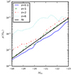 |
Fig. 1. GW host probability as a function of the galaxies’ absolute magnitudes in the K band. Different lines indicate the host probability at different redshifts. The GW host probability is from Artale et al. (2020). |
 (16)
(16)
We show it in Fig. 1 in comparison with the numerical values provided by Artale et al. (2020). Hence, under the approximations done so far, the final merger rate model we consider leads to
 (17)
(17)
We warrant that typically the SFR at low redshift is not separable into two independent terms (Behroozi et al. 2013), namely fSFR(z, L)≠fSFR(z)fSFR(L). As a consequence, if the CBC merger rate perfectly tracks the SFR, our model in Eq. (17) should be revisited as additional biases on H0 could be introduced by the z, L interplay. However, currently, the CBC merger rate as a function of z and L is not measured from data and the simulations of Artale et al. (2020) predicts that the GW host probability can be approximated as fCBC(z, L)≈fCBC(z)fCBC(L), also at low redshift. This can also be appreciated in Fig. 1, obtained from Artale et al. (2020), where we can see that the GW host probability as a function of MKs is different only for sources at z ≳ 5.
3.2. Simulation of the GW catalogue
In Fig. 2 we summarize the steps taken to obtain the GW catalogue from MICEcat. As discussed in Sect. 2, we performed our study by considering several sky localization areas for the GW events. Hence, the first step of the simulation was to filter all the galaxies reported by MICEcat in a given sky location. To do so, we used the python package healpy (Zonca et al. 2019) to divide the sky into equal-sized pixels with the same sky area and then selected all the galaxies falling in each of the LOSs considered. For this study, we considered sky localization areas of 1 deg2, 10 deg2, and 100 deg2 to mimic the typical sky localizations of a network made by three GW detectors (Kagra Collaboration et al. 2018). When dealing with GW events localized within 1 deg2 or 10 deg2 (100 deg2), we considered 100 pixels (60 pixels) randomly distributed in the sky octant.
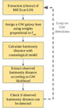 |
Fig. 2. Flowchart of the process to simulate GW events from MICEcat. |
After a LOS was selected, we applied a subsampling of all the galaxies reported by MICEcat. The resampling procedure was applied to speed up the computation of the hierarchical likelihood in Eq. (12); this is required due to the extensive number of runs that we performed. We verified that about ∼3000 galaxies for each LOS are enough to preserve the large-scale structures in redshift from which the Hubble constant is estimated (see Appendix A for more details). After the galaxies were sub-sampled, we calculated for each of them a relative weight using Eq. (6) to host a GW events.
Using the calculated weights, we extracted a galaxy as a host of the GW event, and we computed its luminosity distance, dL, using the true cosmological model. Then we extracted a value of the ‘observed’ luminosity distance,  , using the GW likelihood model in Eq. (4). If the observed luminosity distance is lower than a detection threshold,
  , then we considered the signal as detected. We iterated the procedure described in this section until the desired number of GW sources was obtained.
3.3. Properties of the GW catalogues
Figure 3 shows the distributions of the detected GW events for the three detection thresholds. The first property of the detected population is that the true redshift (luminosity distance) of the sources can extend beyond  . This is because the GW likelihood model can introduce noise fluctuations that make the signals detectable. From Fig. 3 we can also observe that a
  Mpc would result in a population of GW events typically detected within redshift 0.2,
  Mpc within redshift 0.4 and
  Mpc within redshift 1. None of our simulations contains GW sources from galaxies close z ≈ 1.4, which is the cut used to generate MICEcat. As such, our studies do not need to account for the presence of this hard cut in the galaxy distributions.
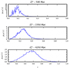 |
Fig. 3. Distribution of detected GW events for different thresholds on the observed luminosity distance and number of detected events. The sky area considered corresponds to a sky-localization of 1 deg2 as an example. |
To quantify better how GWs detected at various distances interact with the construction of the galaxies’ overdensity in the LOS, we computed the single event likelihood,
 (18)
(18)
as a function of the observed distance,  , and conditioned on the true value of
  used to generate MICEcat. The single-likelihood profile can be used to understand how sensitive is the analyses to changes in the prescription of frate. If the likelihood profile as a function of
  is not modified as the prescription of frate changes, then the H0 posterior is not expected to differ. We note that what impacts on the estimation of H0 are changes in the trend of the likelihood and not its overall normalization factor. In Fig. 4 we show this estimator calculated for three different LOSs areas. As we can see from the plots, GW events observed at low distances for small sky areas display large likelihood changes when the galaxy’s luminosity is included in frate. This is because when few galaxies are included in the localization volume, a change in the GW host probability would systematically prefer fewer galaxies, while if many galaxies are included there is no such preference. Instead, a change of prescription of frate as a function of redshift does not affect the single-likelihood as this weight at low redshift is equal for all the galaxies. At higher distances (redshift), the redshift weight in frate causes a more negligible change in the trend of the single event likelihood.
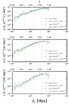 |
Fig. 4. Single-likelihood estimator (vertical axis; see Eq. (18)) as a function of the observed luminosity distance (horizontal axis). The top, middle, and bottom panels were generated assuming that the GW event is localized in a 1 deg2, 10 deg2, and 100 deg2 sky area. The different lines were generated assuming the four prescriptions of frate used in this work and assuming |

4. Forecasting systematics on the H0 inference
In this section we present an extensive study on the systematics that could be introduced in the estimation of H0 when mismodelling the GW host probability, namely the rate function frate. To do so, we simulated 100, 200, and 500 GW detections from MICEcat using the fiducial model for frate in Eq. (8) and we then performed the inference using four different models for frate. The first is the correct one and accounts for both the redshift and absolute magnitude dependence, the second neglects the absolute magnitude, the third the redshift dependence, and the fourth both the absolute magnitude and redshift. In estimating the H0 we used a uniform prior in the range [40, 120] km s−1 Mpc−1.
For each of these cases, we built probability-probability (PP) plots (e.g. Wilk & Gnanadesikan 1968) for the H0 posterior. PP plots were built by repeating each simulation 100 times, each time drawing a value for H0 in the prior range [40, 120] km s−1 Mpc−1. For each posterior obtained, we computed at which credible interval, ℐ, the true value of H0inj is found, namely
 (19)
(19)
If no bias is present, the distribution of the ℐi is expected to be uniform in the range [0,1] and its cumulative (the PP-plot) is expected to be a bisector in the range [0,1].
4.1. Case 1: All GW sources are observed in the same line of sight
We start by discussing a simple case in which all the GW detections are obtained from the same LOS. In this limiting case, the distribution of galaxies, from the GW point of view, will strongly deviate from a uniform in comoving volume distribution. This is due to the fact we are observing GWs from the same LOS that contains always the same anisotropies in the redshift and luminosity distribution of galaxies. Thus, we expect that systematically mismatching frate for the same set of galaxies might introduce a systematic bias on the H0 estimation.
In Fig. 5 we show the PP plots for the various cases that we simulated using a sky localization area of 10 deg2. In all the cases, we find that when frate is modelled correctly, the inference does not show any significant bias, as expected. However, if we consider a detection horizon ≤1550 Mpc (i.e. we observe GW events at small distances), we obtain that mismodelling frate can introduce a significant bias. In particular, we find that if galaxy luminosities are neglected, then the H0 posterior will typically display a bias towards higher values of H0 and that this effect depends on the galaxy distribution along the LOS considered. In fact, from the plots in Fig. 5, we can also observe that this is the dominant source of the bias, even if the redshift dependence of frate is neglected. The magnitude of the H0 bias increases as more GW events are used for the inference as expected for a systematic bias stacking on each of the GW events analysed. If we consider  = 4250 Mpc, we find that mismodelling frate does not introduce any significant bias. We verified that the results obtained for 10 deg2 are also valid for 1 deg2, while for 100 deg2 the bias results weakened since, when considering large volumes, the local anisotropy tends to be averaged out.
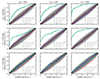 |
Fig. 5. PP plots corresponding to a single LOS covering a sky area of 10 deg2. The rows correspond to the three different thresholds in luminosity distance, the columns to different numbers of detected GW events, NGW. |
The results presented in the previous paragraph can be explained as follows. When  < 1550 Mpc, we are typically dealing with close-by GW events whose luminosity distance uncertainties are low4. As a consequence, they include in their localization volume galaxies distributed in a narrow redshift space but can show some significant anisotropies in terms of luminosity distribution. Therefore, mismatching the dependence of frate from the galaxies’ luminosity introduces a strong bias for the inference while the effect of mismatching the redshift dependence is small. On the other hand, if we have a detection threshold
  = 4250 Mpc, most of the GW events will be located at high distances and will have a large localization volume. As a consequence, they will include galaxies over a wide redshift range but as the redshift range is large, we do not expect to see any significant anisotropy in their distribution in terms of luminosity. It follows that in this case, mismodelling the redshift dependence on frate is more important than mismodelling luminosity dependence. Figure 4 corroborates the above discussion, which shows that the single-event likelihood is different at low redshift when mismatching the luminosity weight and at high redshift when mismatching the redshift dependence.
The behaviour of H0 is directly linked to the type of mismodelling that we are conducting for frate. Remembering that H0 ∝ z/dL, when a bias is introduced by a wrong modelling of the redshift dependence, we systematically set GW hosts at redshifts lower than to their true distribution. This results in a bias towards lower H0 values (also hinted at by the curves in Fig. 5). When we neglect the intrinsic luminosity dependence of frate, we are more likely to assign GW events to faint galaxies and for this particular LOS translates to a high H0 bias. To provide a more qualitative picture of the biases, we show in Fig. 6 the reconstructed posterior for dLthr = 1550 Mpc and 200 detected GWs and with a sky area of 10 deg2, where the true value of H0 has been set to 70 km s−1 Mpc−1. As it can been seen from the plot, the H0 posterior is sensitive to the models of frate. Although for this particular case, the statistical errors are sufficiently large to include the true value of H0, the overall statistical framework suffers from systematic biases as demonstrated by the PP plots.
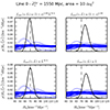 |
Fig. 6. Posterior obtained by fixing H0 to 70 km s−1 Mpc−1 and |

4.2. Case 2: GWs from all sky directions
We repeated the procedure from Sect 4.1 by randomizing the LOS from which each GW event is observed. This procedure is equivalent to assuming that the GW distribution is isotropic in our Universe. In this case we expect the average distribution of galaxies in redshifts over all the LOSs to be reasonably uniform in comoving volume, and thus, any local anisotropy present in the luminosity distribution should be averaged out. In other words, we would expect that when not accounting for the galaxies’ luminosity in frate, the systematic introduced on H0 will be sometimes to the right and sometimes to the left, thus resulting in no bias. When we consider GW events detected at distances of 𝒪(Gpc), mismatching the redshift dependence leads to a further systematic bias, shifting the posterior towards lower values of H0. As explained in the previous section, when the redshift range considered is large, mismodelling the redshift dependence translates in preferring nearer galaxies as GW hosts, hence providing a shift of the posterior to the left.
Figure 7 shows the PP plots for a sky area of 10 deg2. Also in this case, we observe similar behaviours to the ones observed in the previous section: if the CBC rate function as a function of redshift if mismatched, this will result in a bias when considering GW events detected at higher distances. Differently to the single-LOS case, when the intrinsic galaxy luminosity is mismatched, we obtain the posterior on H0 that is typically unbiased, even for close-by and well-localized GW events. This is consistent with the fact that by marginalizing over different LOSs, galaxies’ clustering properties tend to follow a uniform comoving volume distribution that is unaffected by the actual galactic properties. We provide a qualitative picture in Fig. 8, where we show the reconstructed posterior for dLthr = 4250 Mpc and 500 detected GWs and with a sky area of 10 deg2, where the true value of H0 has been set to 70 km s−1 Mpc−1.
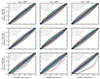 |
Fig. 7. PP plots obtained by taking a different LOS each time when estimating the posterior, each from the chosen 100, covering a sky area of 10 deg2. The rows correspond to the three different luminosity distance thresholds, the columns to different numbers of detected GW events, NGW. |
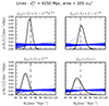 |
Fig. 8. Posterior obtained by fixing H0 to 70 km s−1 Mpc−1 and |

5. Conclusions
We have performed a systematic study on the bias that can be introduced on the inference of H0 for dark sirens cosmology with galaxy catalogues. We performed extensive end-to-end simulations to infer H0 from GW standard sirens starting from MICEcat, a simulated universe that reproduces the large-scale structure properties of our Universe.
Assuming the galaxy catalogue is complete and using a set of simplified assumptions for the GW detection probability and GW localization, we have shown that mismodelling of the CBC host probability, namely frate, can introduce relevant biases when estimating H0. We have found that mismatching the frate dependence as a function of redshift will most likely introduce a systematic shift at low H0 when dealing with hundreds of GW detections detected at luminosity distances greater than 2 Gpc. We have also found that mismatching frate as a function of the galaxy’s luminosities might introduce a systematic bias on H0 when dealing with multiple events from the same LOS detected at very close distances. However, we have shown, for the first time, that when dealing with GW events from different LOSs, even close ones, mismatching the galaxy luminosity dependence on frate is not expected to result in a significant bias on H0.
The results presented in this paper are scalable to other GW detector networks. If we assume that the luminosity distance errors do not strongly change with the SNR5, then the luminosity distance detection thresholds can be rephrased in terms of SNR detection thresholds. Thus, working with luminosity distance thresholds would implicitly mean working with standard sirens selected according to a SNR cut that depends on the detector network. As an example, with current GW detectors, a black hole binary at 500 Mpc would enter the analysis with a SNR cut of ≳40, while for future-generation detectors it would enter the analysis for a SNR cut of ≳103.
We argue that these results are valid, with some caveats. We used more than 100 GW events for the H0 inference. In the case of a low number of GW detections (i.e. a few localized standard sirens with very high SNR), we expect that assumptions on the host galaxy properties might introduce a systematic bias to H0 as, on average, the large-scale structures seen using GW events are not uniform in comoving volume. In other words, a low number of highly localized GW sources would mimic the behaviour observed for the case of 100 well-localized sources drawn from the same LOS.
Morevoer, our results were generated assuming a complete galaxy catalogue in terms of CBC hosts. However, for populations of GW sources at high redshifts, where current catalogues are expected to be incomplete, a bias will most likely be introduced by a mismodelling of the CBC merger rate as a function of redshift. The CBC merger rate as a function of redshift needs to also be modelled for the completeness correction, with the same exact parametrization of frate(z). Therefore, we expect that for this case our results will remain unchanged even if we include the completeness correction. At the same time, we also expect that for close-by GW events, our results will not vary as the galaxy catalogue would be nearly complete. Of course, the level of completeness will strongly depend on the apparent magnitude sensitivities. It is currently unknown how mismatching the completeness correction would result in a systematic bias for catalogues that are not 100% complete. We leave this analysis for more dedicated studies as simulating galaxy catalogue incompleteness involves several survey-specific issues, such as modelling of the Schechter function (including a dependence on the redshift), the definition of realistic apparent magnitude cuts, and colour corrections.
Unless it is sourced by primordial black holes formed at early Universe ages (Sasaki et al. 2018) or it results from the merger of binaries with large kick velocities (Gerosa & Moore 2016). Both types of events are expected to be very rare.
Let us remind the reader that this is a consequence of the fact that we have assumed the GW likelihood uniform in a given sky area.
See Bellomo et al. (2022) for additional details on the integration boundaries.
Remember that in our model the typical luminosity distance uncertainties are of the order of 20% of the luminosity distance.
This is a reasonable assumption if we assume that the luminosity distance inclination degeneracy dominates the GW error budget (Chassande-Mottin et al. 2019).
Acknowledgments
CloudVeneto is acknowledged for the use of computing and storage facilities. A.R. thanks Steven N. Shore for valuable comments on the draft and M. Cignoni for discussions. AR acknowledges financial support from the Italian Ministry of University and Research (MUR) for the PRIN grant METE under contract no. 2020KB33TP and from the Supporting TAlent in ReSearch@University of Padova (STARS@UNIPD) for the project “Constraining Cosmology and Astrophysics with Gravitational Waves, Cosmic Microwave Background and Large-Scale Structure cross-correlations”. SM is supported by ERC Starting Grant No. 101163912–GravitySirens.
References
- Abbott, B. P., Abbott, R., Abbott, T. D., et al. 2016, Phys. Rev. Lett., 116, 061102 [Google Scholar]
- Abbott, B. P., Abbott, R., Abbott, T. D., et al. 2017a, Phys. Rev. Lett., 119, 161101 [Google Scholar]
- Abbott, B. P., Abbott, R., Abbott, T. D., et al. 2017b, ApJ, 848, L12 [Google Scholar]
- Abbott, R., Abbott, T. D., Abraham, S., et al. 2021a, ApJ, 913, L7 [NASA ADS] [CrossRef] [Google Scholar]
- Abbott, B. P., Abbott, R., Abbott, T. D., et al. 2021b, ApJ, 909, 218 [NASA ADS] [CrossRef] [Google Scholar]
- Abbott, R., Abbott, T. D., Abraham, S., et al. 2021c, Phys. Rev. D, 104, 022004 [NASA ADS] [CrossRef] [Google Scholar]
- Abbott, R., Abbott, T. D., Acernese, F., et al. 2023a, Phys. Rev. X, 13, 011048 [NASA ADS] [Google Scholar]
- Abbott, R., Abe, H., Acernese, F., et al. 2023b, ApJ, 949, 76 [NASA ADS] [CrossRef] [Google Scholar]
- Artale, M. C., Bouffanais, Y., Mapelli, M., et al. 2020, MNRAS, 495, 1841 [Google Scholar]
- Auclair, P., Bacon, D., Baker, T., et al. 2023, Living Rev. Rel., 26, 5 [Google Scholar]
- Behroozi, P. S., Wechsler, R. H., & Conroy, C. 2013, ApJ, 770, 57 [NASA ADS] [CrossRef] [Google Scholar]
- Bellomo, N., Bertacca, D., Jenkins, A. C., et al. 2022, JCAP, 06, 030 [Google Scholar]
- Bera, S., Rana, D., More, S., & Bose, S. 2020, ApJ, 902, 79 [NASA ADS] [CrossRef] [Google Scholar]
- Borghi, N., Mancarella, M., Moresco, M., et al. 2024, ApJ, 964, 191 [Google Scholar]
- Branchesi, M., et al. 2023, JCAP, 07, 068 [CrossRef] [Google Scholar]
- Carretero, J., Castander, F. J., Gaztañaga, E., Crocce, M., & Fosalba, P. 2015, MNRAS, 447, 646 [NASA ADS] [CrossRef] [Google Scholar]
- Chassande-Mottin, E., Leyde, K., Mastrogiovanni, S., & Steer, D. A. 2019, Phys. Rev. D, 100, 083514 [Google Scholar]
- Chen, H.-Y., Fishbach, M., & Holz, D. E. 2018, Nature, 562, 545 [Google Scholar]
- Chernoff, D. F., & Finn, L. S. 1993, ApJ, 411, L5 [Google Scholar]
- Crocce, M., Castander, F. J., Gaztañaga, E., Fosalba, P., & Carretero, J. 2015, MNRAS, 453, 1513 [NASA ADS] [CrossRef] [Google Scholar]
- Dalal, N., Holz, D. E., Hughes, S. A., & Jain, B. 2006, Phys. Rev. D, 74, 063006 [Google Scholar]
- Del Pozzo, W. 2012, Phys. Rev. D, 86, 043011 [NASA ADS] [CrossRef] [Google Scholar]
- Essick, R., & Fishbach, M. 2024, Astrophys. J., 962, 169 [Google Scholar]
- Evans, M., Adhikari, R. X., Afle, C., et al. 2021, ArXiv e-prints [arXiv:2109.09882] [Google Scholar]
- Ezquiaga, J. M., & Holz, D. E. 2021, ApJ, 909, L23 [CrossRef] [Google Scholar]
- Ezquiaga, J. M., & Holz, D. E. 2022, Phys. Rev. Lett., 129, 061102 [NASA ADS] [CrossRef] [Google Scholar]
- Farr, W. M. 2019, RNAAS, 3, 66 [Google Scholar]
- Finke, A., Foffa, S., Iacovelli, F., Maggiore, M., & Mancarella, M. 2021, JCAP, 08, 026 [Google Scholar]
- Fishbach, M., Holz, D. E., & Farr, W. M. 2018, ApJ, 863, L41 [NASA ADS] [CrossRef] [Google Scholar]
- Fishbach, M., Gray, R., Magaña Hernandez, I., et al. 2019, ApJ, 871, L13 [NASA ADS] [CrossRef] [Google Scholar]
- Fosalba, P., Crocce, M., Gaztañaga, E., & Castander, F. J. 2015a, MNRAS, 448, 2987 [NASA ADS] [CrossRef] [Google Scholar]
- Fosalba, P., Gaztañaga, E., Castander, F. J., & Crocce, M. 2015b, MNRAS, 447, 1319 [NASA ADS] [CrossRef] [Google Scholar]
- Gair, J. R., Ghosh, A., Gray, R., et al. 2023, AJ, 166, 22 [NASA ADS] [CrossRef] [Google Scholar]
- Galbany, L., de Jaeger, T., Riess, A. G., et al. 2023, A&A, 679, A95 [NASA ADS] [CrossRef] [EDP Sciences] [Google Scholar]
- Gerosa, D., & Moore, C. J. 2016, Phys. Rev. Lett., 117, 011101 [Google Scholar]
- Gray, R., Magaña Hernandez, I., Qi, H., et al. 2020, Phys. Rev. D, 101, 122001 [NASA ADS] [CrossRef] [Google Scholar]
- Gray, R., Messenger, C., & Veitch, J. 2022, MNRAS, 512, 1127 [NASA ADS] [CrossRef] [Google Scholar]
- Gray, R., Beirnaert, F., Karathanasis, C., et al. 2023, JCAP, 2023, 023 [CrossRef] [Google Scholar]
- Hanselman, A. G., Vijaykumar, A., Fishbach, M., & Holz, D. E. 2025, ApJ, 979, 9 [Google Scholar]
- Hoffmann, K., Bel, J., Gaztañaga, E., et al. 2015, MNRAS, 447, 1724 [NASA ADS] [CrossRef] [Google Scholar]
- Holz, D. E., & Hughes, S. A. 2005, ApJ, 629, 15 [Google Scholar]
- Kagra Collaboration, Ligo Scientific Collaboration,& VIRGO Collaboration (Abbott, B. P., et al.) 2018, Liv. Rev. Relat., 21, 3 [NASA ADS] [CrossRef] [Google Scholar]
- Karathanasis, C., Mukherjee, S., & Mastrogiovanni, S. 2023, MNRAS, 523, 4539 [NASA ADS] [Google Scholar]
- Leandro, H., Marra, V., & Sturani, R. 2022, Phys. Rev. D, 105, 023523 [Google Scholar]
- Leyde, K., Mastrogiovanni, S., Steer, D. A., Chassande-Mottin, E., & Karathanasis, C. 2022, JCAP, 09, 012 [CrossRef] [Google Scholar]
- Madau, P., & Dickinson, M. 2014, Annu. Rev. Astron. Astrophys., 52, 415 [Google Scholar]
- Maggiore, M., Van Den Broeck, C., Bartolo, N., et al. 2020, JCAP, 03, 050 [CrossRef] [Google Scholar]
- Mandel, I., Farr, W. M., & Gair, J. R. 2019, MNRAS, 486, 1086 [Google Scholar]
- Mastrogiovanni, S., Leyde, K., Karathanasis, C., et al. 2021, Phys. Rev. D, 104, 062009 [NASA ADS] [CrossRef] [Google Scholar]
- Mastrogiovanni, S., Laghi, D., Gray, R., et al. 2023, Phys. Rev. D, 108, 042002 [NASA ADS] [CrossRef] [Google Scholar]
- Mastrogiovanni, S., Pierra, G., Perriès, S., et al. 2024, A&A, 682, A167 [NASA ADS] [CrossRef] [EDP Sciences] [Google Scholar]
- Mukherjee, S. 2022, MNRAS, 515, 5495 [NASA ADS] [CrossRef] [Google Scholar]
- Mukherjee, S., Wandelt, B. D., & Silk, J. 2020, MNRAS, 494, 1956 [Google Scholar]
- Mukherjee, S., Wandelt, B. D., Nissanke, S. M., & Silvestri, A. 2021, Phys. Rev. D, 103, 043520 [CrossRef] [Google Scholar]
- Oguri, M. 2016, Phys. Rev. D, 93, 083511 [Google Scholar]
- Palmese, A., deVicente, J., Pereira, M. E. S., et al. 2020, ApJ, 900, L33 [Google Scholar]
- Palmese, A., Bom, C. R., Mucesh, S., & Hartley, W. G. 2023, ApJ, 943, 56 [NASA ADS] [CrossRef] [Google Scholar]
- Planck Collaboration VI. 2020, A&A, 641, A6 [Erratum: A&A, 652, C4 (2021)] [NASA ADS] [CrossRef] [EDP Sciences] [Google Scholar]
- Sasaki, M., Suyama, T., Tanaka, T., & Yokoyama, S. 2018, CQGra, 35, 063001 [Google Scholar]
- Schutz, B. F. 1986, Nature, 323, 310 [Google Scholar]
- Sivia, D., & Skilling, J. 2006, Data Analysis: A Bayesian Tutorial (OUP Oxford) [CrossRef] [Google Scholar]
- Soares-Santos, M., Palmese, A., Hartley, W., et al. 2019, ApJ, 876, L7 [NASA ADS] [CrossRef] [Google Scholar]
- Taylor, S. R., Gair, J. R., & Mandel, I. 2012, Phys. Rev. D, 85, 023535 [Google Scholar]
- Vijaykumar, A., Fishbach, M., Adhikari, S., & Holz, D. E. 2024, ApJ, 972, 157 [Google Scholar]
- Vitale, S., Gerosa, D., Farr, W. M., & Taylor, S. R. 2020, ArXiv e-prints [arXiv:2007.05579] [Google Scholar]
- Wilk, M. B., & Gnanadesikan, R. 1968, Biometrika, 55, 1 [Google Scholar]
- Zonca, A., Singer, L., Lenz, D., et al. 2019, J. Open Source Softw., 4, 1298 [Google Scholar]
Appendix A: Sub-sampling of the lines of sight
To ease the computational burden of the analyses, we sub-sampled the galaxies reported in every MICEcat LOS. We empirically find that a subsampling of about ∼3000 galaxies does not modify the statistical properties of the galaxies’ distribution. We report in Fig. A.1 the comparison between the redshift (blue) and absolute magnitude (in orange) for the sub-sampled data with the full data (black) for the different sky areas we considered. We quantified the difference between the original and sub-sampled distributions using the discrete Kullback-Leibler divergence calculated by subdividing the redshift and magnitude ranges in 20 bins. We find the Kullback-Leibler divergence to be at most 10−1. Hence, we considered the sub-sampled and the full distributions to be statistically indistinguishable.
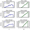 |
Fig. A.1. Comparison of the distribution of redshifts (left column) and magnitudes (right column) between original galaxies for some selected LOSs in MICEcat and the sub-sampled ones. The rows report sky areas of respectively 1 deg2, 10 deg2, and 100 deg2. |
All Figures
|
Fig. 1. GW host probability as a function of the galaxies’ absolute magnitudes in the K band. Different lines indicate the host probability at different redshifts. The GW host probability is from Artale et al. (2020). |
| In the text | |
|
Fig. 2. Flowchart of the process to simulate GW events from MICEcat. |
| In the text | |
|
Fig. 3. Distribution of detected GW events for different thresholds on the observed luminosity distance and number of detected events. The sky area considered corresponds to a sky-localization of 1 deg2 as an example. |
| In the text | |
|
Fig. 4. Single-likelihood estimator (vertical axis; see Eq. (18)) as a function of the observed luminosity distance (horizontal axis). The top, middle, and bottom panels were generated assuming that the GW event is localized in a 1 deg2, 10 deg2, and 100 deg2 sky area. The different lines were generated assuming the four prescriptions of frate used in this work and assuming |
| In the text | |
|
Fig. 5. PP plots corresponding to a single LOS covering a sky area of 10 deg2. The rows correspond to the three different thresholds in luminosity distance, the columns to different numbers of detected GW events, NGW. |
| In the text | |
|
Fig. 6. Posterior obtained by fixing H0 to 70 km s−1 Mpc−1 and |
| In the text | |
|
Fig. 7. PP plots obtained by taking a different LOS each time when estimating the posterior, each from the chosen 100, covering a sky area of 10 deg2. The rows correspond to the three different luminosity distance thresholds, the columns to different numbers of detected GW events, NGW. |
| In the text | |
|
Fig. 8. Posterior obtained by fixing H0 to 70 km s−1 Mpc−1 and |
| In the text | |
|
Fig. A.1. Comparison of the distribution of redshifts (left column) and magnitudes (right column) between original galaxies for some selected LOSs in MICEcat and the sub-sampled ones. The rows report sky areas of respectively 1 deg2, 10 deg2, and 100 deg2. |
| In the text | |
Current usage metrics show cumulative count of Article Views (full-text article views including HTML views, PDF and ePub downloads, according to the available data) and Abstracts Views on Vision4Press platform.
Data correspond to usage on the plateform after 2015. The current usage metrics is available 48-96 hours after online publication and is updated daily on week days.
Initial download of the metrics may take a while.