| Issue |
A&A
Volume 697, May 2025
|
|
|---|---|---|
| Article Number | A199 | |
| Number of page(s) | 9 | |
| Section | Stellar structure and evolution | |
| DOI | https://doi.org/10.1051/0004-6361/202553749 | |
| Published online | 19 May 2025 | |
Binary evolution pathways to blue large-amplitude pulsators: Insights from HD 133729
1
Yunnan Observatories, Chinese Academy of Sciences, Kunming 650011, PR China
2
University of the Chinese Academy of Sciences, 19A Yuquan Road, Shijingshan District, Beijing 100049, PR China
3
International Centre of Supernovae, Yunnan Key Laboratory, Kunming 650216, PR China
4
Institute for Frontier in Astronomy and Astrophysics, Beijing Normal University Beijing 102206, PR China
5
Department of Astronomy, Beijing Normal University, Beijing 100875, PR China
⋆ Corresponding authors: This email address is being protected from spambots. You need JavaScript enabled to view it.
; This email address is being protected from spambots. You need JavaScript enabled to view it.
Received:
14
January
2025
Accepted:
14
April
2025
Abstract
Blue large-amplitude pulsators (BLAPs) are a recently identified class of pulsating stars distinguished by their short pulsation periods (2–60 minutes) and asymmetric light curves. This study investigated the evolutionary channel of HD 133729, which is the first confirmed BLAP in a binary system. Using the binary evolution code MESA, we explored various mass ratios and initial orbital periods. Our simulations suggest that a system with a mass ratio q = 0.30 undergoing non-conservative mass transfer (β = 0.15) can reproduce the observed characteristics through the pre-white-dwarf Roche lobe overflow channel. Meanwhile, we postulate that there are significant helium and nitrogen enhancements on the surface of the main sequence (MS) star. The system will eventually undergo the common envelope phase, leading to a stellar merger. HD 133729 is a unique case, providing crucial insights into the formation mechanism and evolutionary fate of BLAPs with MS companions. This work constrains the elemental abundances of the MS star and has advanced our understanding of non-conservative mass transfer in binary evolution.
Key words: asteroseismology / binaries: general
© The Authors 2025
 Open Access article, published by EDP Sciences, under the terms of the Creative Commons Attribution License (https://creativecommons.org/licenses/by/4.0), which permits unrestricted use, distribution, and reproduction in any medium, provided the original work is properly cited.
This article is published in open access under the Subscribe to Open model. This email address is being protected from spambots. You need JavaScript enabled to view it. to support open access publication.
1. Introduction
Blue large-amplitude pulsators (BLAPs) are a class of pulsating stars that was first observed by the Optical Gravitational Lensing Experiment (OGLE) survey in 2013 (e.g. Pietrukowicz et al. 2013). BLAPs are characterized by short pulsation periods (22–40 minutes) and asymmetric light curves. These light curves show a rapid rise followed by a slower decline in brightness (e.g. Pietrukowicz et al. 2017). BLAPs occupy a region on the Hertzsprung-Russell (HR) diagram between hot massive main sequence (MS) stars and hot subdwarfs. Their luminosities (log(L/L⊙) = 2.2 − 2.6) are approximately an order of magnitude higher than those of hot subdwarfs, whereas their surface gravities (log(g/cm s−2) = 4.5 − 4.8) are significantly lower. In addition to typical BLAPs, there is also a class of high-gravity BLAPs whose spectroscopic properties and pulsation periods are more similar to those of subdwarf B-type (sdB) stars pulsating in the p-mode, with Teff ≃ 32 000 K and pulsation periods between 200 and 475 seconds (e.g. Kupfer et al. 2019; Meng et al. 2020; Ramsay et al. 2022; McWhirter & Lam 2022; Borowicz et al. 2023; Bradshaw et al. 2024; Chang et al. 2024).
The pulsation mechanism of BLAPs is attributed to the κ mechanism and is driven by the iron opacity bump at a specific temperature. The phenomenon of radiative levitation arises from the outward force exerted by stellar radiation on ions within a star. This phenomenon was originally proposed to explain the pulsations observed in hot subdwarf stars (e.g. Charpinet et al. 1996; Hu et al. 2011; Jeffery & Saio 2016). Byrne & Jeffery (2018) highlighted the significant role of radiative levitation, which leads to the accumulation of iron and nickel around a temperature of ≃2 × 10⁵ K. This accumulation forms a substantial opacity bump that drives the pulsations observed in BLAPs.
Several models have been proposed to explain the origin of BLAPs (also see Fig. 1):
-
Low-mass pre-white-dwarf model: This model proposes that BLAPs originate from low-mass stars (typically 0.2–0.4 M⊙) formed through significant mass loss from a red giant star in a binary system. This mass loss occurs via common envelope (CE) evolution or Roche lobe overflow (RLOF; e.g. Romero et al. 2018; Byrne & Jeffery 2018; Córsico et al. 2018; Byrne et al. 2021). During the BLAP phase, these stars possess helium cores with residual hydrogen shell burning, which sustains their high effective temperatures and luminosities. They are in a pre-white-dwarf evolutionary stage, en route to becoming white dwarfs (WDs).
-
Helium-burning models: (a) Core helium-burning star. This scenario suggests that BLAPs evolve from stars with initial masses higher than 4.0 M⊙, potentially as surviving companions of Type Ia supernovae. The common envelope wind model posits that such companions lose mass in a binary system, leading to their current configuration (e.g. Wu & Li 2018; Meng et al. 2020). In their BLAP phase, these stars have masses between 0.5 and 1.2 M⊙ and are undergoing core helium burning, with thin hydrogen envelopes contributing to their observed properties. (b) Shell helium-burning star. BLAPs may form in long-period binary systems through stable RLOF, during which mass transfer from a companion shapes their evolution. During this phase, they are shell helium-burning sdB stars, exhibiting the pulsational and photometric characteristics of BLAPs (e.g. Xiong et al. 2022).
-
BLAPs can arise from two distinct merger scenarios: (a) A merger of a He WD with a low-mass MS star. This process produces a hot subdwarf that evolves through a BLAP-like state (e.g. Zhang et al. 2023). (b) A merger of two extremely low-mass WDs. Systems with total masses between 0.32 and 0.7 M⊙ merge to form a single object that rapidly enters the BLAP phase after coalescence (e.g. Kołaczek-Szymański et al. 2024). The merger process can also generate strong magnetic fields, explaining magnetic BLAPs (e.g. Pigulski et al. 2024). For a He WD + MS merger, the star passes through this state between helium shell ignition and core burning. For a merger of two extremely low-mass WDs, the merged object remains in the BLAP phase for 20 000–70 000 years, displaying BLAP characteristics before evolving into hot subdwarfs and eventually into He WDs or hybrid He–CO WDs.
Although more than 80 BLAPs have been discovered, very few have been confirmed as binary systems (e.g. Pietrukowicz et al. 2024). TMTS-BLAP-1 is potentially a wide binary system with an orbital period of 1576 days, but this has not yet been confirmed (e.g. Lin et al. 2023). Recent photometric analysis has revealed that HD 133729 is a binary system. It consists of a late B-type MS star and a BLAP companion. This makes HD 133729 the first, and currently the only, confirmed BLAP in a binary system. Analysis of TESS data from both sectors revealed a dominant frequency at fP = 44.486 d−1, which corresponds to a pulsation period of 32.37 minutes. Harmonics were also observed, indicating a non-sinusoidal light curve, a characteristic feature of BLAPs. The light-travel-time effect manifests as orbital sidelobes in the frequency spectra. While the sidelobe separation of approximately 0.043 d−1 in the TESS Fourier transform (FT) suggests an orbital period of  days, a more precise determination using the O–C diagram from WASP and TESS data confirms an orbital period of 23.08433 ± 0.00023 days, providing a stronger detection than the TESS FT sidelobes alone (e.g. Pigulski et al. 2022). Additional observational data are provided in Table 1. It should be noted that the log(g) = 4.5 of the BLAP was assumed to fit a model spectral energy distribution to the single far-ultraviolet data point; it is consistent with the other BLAP parameters listed in Table 1.
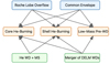 |
Fig. 1. Schematic diagram for the origin of BLAPs. The starting point of the arrow indicates the stellar evolutionary pathway, while the end represents the star’s evolutionary state. |
Observational data of HD 133729.
Questions remain about the BLAP in the HD 133729 system regarding its origin, current state, and later evolution. Did it form through mass loss in a binary via CE or RLOF? Is it now a low-mass pre-WD or a helium-burning star? How do the surface abundances of the B-type MS star compare to those of single MS stars? Could any abundance anomalies be used as diagnostic tools in spectroscopic analyses? Finally, was the mass transfer in HD 133729 conservative or non-conservative? HD 133729 offers a unique opportunity to investigate the formation and evolution of BLAPs. This study focuses on the evolutionary pathways of BLAPs with MS companions. HD 133729 serves as a prototype for this investigation.
This paper is structured as follows. In Sect. 2 we show the methods and parameters used for our stellar evolution and pulsation calculations. Section 3 presents the evolutionary outcomes, categorized by mass ratio. A discussion of these results is provided in Sect. 4. Finally, Sect. 5 summarizes the key findings of this study.
2. Methods and numerical input
To investigate the origin of HD 133729, we used MESA (version r23.05.1) to simulate the evolution of binary systems (e.g. Paxton et al. 2011, 2013, 2015, 2018, 2019). The ‘binary’ module in MESA evolves binary systems by creating two single stars using the ‘star’ module. This module can evolve a primary star with a point-mass companion or evolve both stars simultaneously. The latter approach was adopted (e.g. Paxton et al. 2015).
First, we created a series of pre-MS stellar models using the create_pre_main_sequence_model in the star module, as shown in Table 2. We used a metallicity of Z = 0.02 for all models. For opacity, we selected the GS98 table (e.g. Grevesse & Sauval 1998). For convection, we applied the standard mixing length theory (MLT) with αMLT = 2 (Zhang et al. 2024). We did not include the effects of convective overshooting, thermohaline mixing, or semi-convection.
Initial parameters for binary evolution.
We then added the primary and secondary stars to the binary module. The mass transfer process follows the Ritter prescription (e.g. Ritter 1988). This prescription predicts that matter flows through the inner Lagrangian point L1 as an isothermal, subsonic gas stream. As the stream approaches L1, it reaches the speed of sound. We set the eccentricity of the system to the observed value of e = 0.0055, corresponding to a nearly circular orbit.
We examined both conservative and non-conservative evolution. In the conservative case, the system transfers mass between stars without additional mass loss from rapid stellar winds. In the case of non-conservative evolution, mass is lost from the system alongside the transfer of interstellar mass. In systems with low mass transfer efficiency, angular momentum loss is described by the model of Soberman et al. (1997), in which a fixed fraction of the transferred mass is expelled either as fast, isotropic stellar winds from each star or as circumbinary material forming a ring at a specified radius. The accreted fraction of mass is defined as ϵw ≡ 1 − α − β. Here, α represents the fraction of mass lost as stellar winds and β is the fraction isotropically re-emitted. We tested various β values to analyse their impact on mass evolution and to match observed properties.
The pulsation period was calculated using the following formula (Eddington 1918):
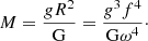 (1)
(1)
This equation relates the mass of the star to its surface gravity, radius, and pulsation frequency. The parameter f = ω/ωdyn, where ωdyn2 = GM/R3 is the dynamical frequency of the star. For low-mass helium-core pre-WD models, f ≈ 3.6. G is the gravitational constant (e.g. Kupfer et al. 2019).
Byrne et al. (2021) found no strong correlation between the initial and final masses of BLAPs. This finding indicates that other binary parameters, such as the mass ratio and the initial orbital period, play a more significant role in determining the final mass. Consequently, we computed evolutionary models over various mass ratios and orbital periods.
3. Results
The formation and evolution of the BLAP progenitor in HD 133729 can be explained by two binary formation channels: the pre-WD RLOF/CE channel, and the helium-burning RLOF/CE channel. Both channels involve binary interaction. In HD 133729, the B-type MS star has a mass of (2.85 ± 0.25) M⊙, indicating that the original progenitor of the BLAP in HD 133729 must have been the primary star.
If the progenitor evolved through the helium-burning channel, it would have undergone significant mass loss. Since a zero-age main sequence (ZAMS) star requires at least 4 M⊙ to eventually become a BLAP, roughly 3.5 M⊙ would need to be removed to form a helium-burning star. Under the assumption of conservative mass transfer, the secondary star should have accreted enough mass to exceed 3.5 M⊙. This contradicts the observed mass of the B-type MS star in HD133729, rendering the helium-burning channel unlikely for this system.
Our calculations further reveal that, for the pre-WD channel, systems with initial orbital periods longer than 100 days exhibit a rapid increase in the mass transfer rate – exceeding 10−3 M⊙ yr−1 – once the donor fills its Roche lobe. This rapid mass transfer triggers CE. In these scenarios, the minimum required CE efficiency (αCE) for successful envelope ejection exceeds 10, implying that these systems will likely merge. Therefore, our study focuses exclusively on the RLOF pre-WD channel for HD133729.
3.1. Cases for q = 0.25
For q = 0.25 and an initial orbital period of 1.0 day, the primary star begins mass transfer while still on the MS. Its core hydrogen abundance is between 0.17 and 0.21, depending on the masses of the binary components. During this phase, the mass transfer timescale (τMT ≈ 106.5 yr) gradually decreases and eventually becomes shorter than the thermal timescale (τKH ≈ 106 yr). Nonetheless, mass accretion can still be maintained.
When the orbital period decreases to approximately 0.5 days, the mass transfer timescale drops suddenly to τMT ≈ 104.2 yr. This further increases the discrepancy between τMT and τKH. As illustrated in Fig. 2 – which shows cases with the highest binary masses – the mass transfer rate becomes extremely high, around 10−4 M⊙ yr−1. Such a rapid rate may trigger a CE phase.
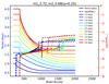 |
Fig. 2. Evolution tracks of a binary system consisting of a M1 = 2.72 M⊙ primary and a M2 = 0.68 M⊙ companion. The x-axis shows the model number. Solid lines represent the orbital period (left y-axis) and dashed lines the logarithm of the mass transfer rate (right y-axis). Different colours correspond to initial orbital periods ranging from 1.0 to 4.0 days. |
A longer orbital period delays the onset of mass transfer. This delay leads to a lower hydrogen abundance in the primary star. However, as in the case with an orbital period of 1.0 days, the accretion rate increases dramatically once the orbital period shrinks to its minimum. This sudden increase suggests that the system is transitioning to a CE phase. Figure 2 shows that even when the orbital period is increased to 4 days, the system behaves similarly. In this scenario, the accretion rate abruptly rises to nearly 10−3 M⊙ yr−1. These results indicate that systems with a mass ratio of q = 0.25 cannot undergo stable mass transfer, thus ruling out this scenario for HD 133729.
3.2. Cases for q = 0.35
We simulated a binary system with a primary star of 2.14 M⊙ and a secondary star of 0.75 M⊙. The system has an orbital period of 1 day. In our simulations, we achieved stable mass transfer with a rate of approximately 10−6 Ṁ yr−1 until the primary star’s mass decreased to 0.73 M⊙ and the secondary star’s mass increased to 2.0 M⊙. At that stage, the secondary star had exhausted its core hydrogen. However, observations of HD 133729 indicate that the companion is a MS star. This result shows that our model does not satisfy the observational requirements. Even when we increased the masses of both stars (up to their maximum plausible values), the secondary star still evolved off the MS, leading to a similar outcome.
The situation differs when the orbital period increases. Figure 3 shows the evolution of systems with a primary star of 2.14 M⊙ and a secondary star of 0.75 M⊙. For initial orbital periods of 1.3–2.5 days, RLOF begins once the primary star exhausts its core hydrogen and enters the Hertzsprung gap. During mass transfer, the secondary star grows to a mass of 2.61–2.63 M⊙ while it remains on the MS. For systems with initial orbital periods between 2.8 and 4.0 days, the mass transfer rate quickly reaches 10−3.8 M⊙ yr−1. This high rate indicates that the binary system likely enters a CE phase as soon as mass transfer begins. Table 3 summarizes the complete evolutionary parameters for binary systems with a mass ratio q = 0.35 undergoing RLOF.
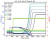 |
Fig. 3. Same as Fig. 2 but for a binary system consisting of a M1 = 2.14 M⊙ primary and a M2 = 0.75 M⊙ companion. |
Parameters for stable mass transfer models at q = 0.35.
Figure 4 shows all cases with q = 0.35 in which the secondary star remains on the MS after mass transfer. Only the system with the highest initial masses (M1 = 2.52 M⊙ and M2 = 0.88 M⊙) and initial orbital periods between 2.2 and 3.4 days shows the primary star’s evolutionary track crossing the BLAP region. However, even when the primary star crosses the BLAP region, calculations show that the pulsation period remains below 32.37 minutes, which is inconsistent with observations. These results indicate that a q = 0.35 cannot explain the observed BLAP.
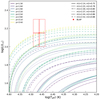 |
Fig. 4. HR diagram for all RLOF channel models with a mass ratio of 0.35. Different line styles represent different binary masses, and different colours represent different initial orbital periods. |
3.3. Cases for q = 0.45
The binary evolution at this mass ratio is similar to the evolution observed for q = 0.35. Assuming that the initial orbital period is Pi (days) = 1.0 for all masses, the primary star begins mass transfer during its MS phase. Accretion by the secondary star accelerates its evolution. Accretion by the secondary star accelerates its evolution, and by the time the secondary exhausts its core hydrogen, the primary retains approximately 0.03 M⊙ of hydrogen. This is inconsistent with the observed evolutionary state of the BLAP in HD 133729.
Mass transfer via RLOF can occur at longer initial orbital periods. We considered a representative system with initial masses M1,i = 2.00 M⊙ and M2,i = 0.90 M⊙. For initial orbital periods Pi between 1.3 and 2.2 days, mass transfer is initiated when the primary star leaves the MS and enters the Hertzsprung gap. In contrast, the secondary remains on the MS. As a result, mass transfer reduces the primary to a pre–WD with a mass in the range 0.265–0.282 M⊙, while the secondary’s mass increases to between 2.618 and 2.635 M⊙; it also remains on the MS. However, the primary’s later evolutionary track on the HR diagram lies below the typical BLAP region.
For systems with initial orbital periods between 2.5 and 4.0 days, mass transfer begins during the Hertzsprung gap phase. However, the mass transfer rate quickly reaches approximately 10−3.76 M⊙ yr−1, indicating the onset of a CE phase. Increasing the total system mass produces results similar to those in Fig. 4; even the highest-mass configurations do not yield pulsation periods that match the observed BLAP characteristics. Table 4 summarizes all instances in which RLOF occurs and the secondary star remains on the MS following mass transfer.
Parameters for stable mass transfer at q = 0.45.
3.4. Cases for q = 0.30
3.4.1. From the ZAMS to BLAP
For models with an initial orbital period of 1 day, mass transfer commences before the primary star completes core hydrogen burning, and the orbital period decreases during this process. At the orbital period minimum, the accretion rate abruptly increases to approximately 10−4 M⊙ yr−1, consistent with the case of q = 0.25 shown in Fig. 2, suggesting the onset of a CE phase. For the two binary model sets with the highest initial masses (the last two in Table 5) and an initial orbital period of 1.3 days, the evolutionary path differs from that of models with q = 0.35 and q = 0.45, as RLOF does not occur. In these cases, mass transfer begins before the primary star completes core hydrogen burning, leaving between 0.04 and 0.06 of its core hydrogen unburnt. At the orbital period minimum, the accretion rate abruptly increases to approximately 10−3.9 M⊙ yr−1, potentially signaling the onset of a CE phase.
Parameters for stable mass transfer at q = 0.30.
We focused on models with orbital periods longer than 1 day. As an illustrative example, we considered the binary system with the lowest total mass, where M1 = 2.23 M⊙ and M2 = 0.67 M⊙. For an initial orbital period between 1.3 and 2.5 days, the stars complete core hydrogen burning and then enter the Hertzsprung gap phase. Subsequently, they fill their Roche lobes, initiating mass transfer via RLOF. Initially, the orbital period decreases until it reaches a minimum, after which the primary and secondary masses reverse. After this reversal, the orbital period increases, and the radius of the primary star shrinks significantly so that it no longer fills its Roche lobe. Consequently, mass transfer ceases. After mass transfer, M1 is reduced to 0.259–0.284 M⊙, M2 increases to 2.616–2.641 M⊙, and the orbital period expands to 12.28–20.38 days. The post-mass transfer parameters for more massive binaries are listed in Table 5. Models with orbital periods outside this range likely entered a CE phase because the initial mass transfer rate was excessively high. This behaviour is similar to that shown in Fig. 3.
Although we identified RLOF models, they do not yet accurately reproduce the observed final orbital and pulsation periods of HD133729. The observed orbital period of the binary system HD133729 is 23.08 days. To identify the best-fitting models, we plotted the initial versus final orbital periods for the last four model sets (Table 5), as shown in Fig. 5, and applied a polynomial fit to determine the best-fit orbital period. We identified four models whose final orbital periods are approximately 23.08 days. Subsequently, we plotted these binary systems on the HR diagram (Fig. 6). We find that models with M1 masses of 2.46 M⊙, 2.54 M⊙, and 2.62 M⊙ all pass through the BLAP region. However, the effective temperatures of the MS stars are higher than the observed values. We address this discrepancy in the next section.
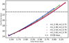 |
Fig. 5. Relationship between final and initial orbital periods for binary systems with mass ratio q = 0.30. Polynomial fits are applied to the four datasets. The horizontal dashed black line represents a final orbital period of 23.08 days. |
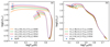 |
Fig. 6. Evolutionary tracks on the HR diagram for binary systems with optimal initial orbital periods derived from polynomial fits. Panel a: Evolutionary paths of the primary stars from the ZAMS through the BLAP phase. Panel b: Corresponding evolutionary tracks of the secondary stars. |
As shown in Fig. 7, two models, with M1 = 2.54 M⊙ and M1 = 2.62 M⊙, respectively, fall within the log Teff range of BLAPs and satisfy the corresponding log(g) criteria. However, only the model with M1 = 2.62 M⊙ reaches a pulsation period of 32.37 minutes within the log Teff region characteristic of BLAPs. Next, we compared the relative rate of period change. The observed value is given by r ≡ ṖP/P = (− 11.5 ± 0.6) × 10−7 yr−1. At a pulsation period of 32.37 minutes, the calculated value is r ≡ ṖP/P = − 1.9 × 10⁻⁶ yr−1. These two values differ by approximately one order of magnitude.
 |
Fig. 7. Diagnostic diagrams showing the evolution of stellar parameters for four binary models selected based on their final orbital period. Panel a: Relationship between effective temperature and surface gravity, with horizontal and vertical dashed lines indicating the observational constraints for BLAP (red: log Teff range; dark blue: log(g/cm s−2) = 4.5). Panel b: Correlation between effective temperature and pulsation period. The horizontal and vertical dashed lines mark the observed BLAP temperature range (red) and the target pulsation period of 32.27 minutes (dark blue), respectively. |
This model offers a compelling explanation for the observed properties of HD 133729. First, the primary star evolves through the BLAP region on the HR diagram; during this process, the model predicts that the pulsation period reaches 32.27 minutes. Second, the primary star attains a surface gravity of log(g/cm s−2) = 4.5 during its traverse of the HR diagram. Third, the model predicts a relative rate of period change of −1.9 × 10⁻⁶ yr−1 at a pulsation period of 32.27 minutes.
3.4.2. Consider the β value in the mass transfer processes
Given that the log Teff of the B-type MS star in the previous model calculations was approximately 1400 K higher than the observed value (Fig. 6), we hypothesized that the mass transfer process was non-conservative. This speculation is reasonable and allows us to define
 (2)
(2)
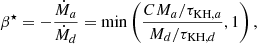
where τKH is the Kelvin-Helmholtz timescale, Ṁd is the mass-loss rate of the donor star, Ṁa is the mass-accretion rate onto the accretor, and C accounts for the increase in the maximum accretion rate due to the expansion of the accreting star (e.g. Paczyński & Sienkiewicz 1972; Neo et al. 1977; Hurley et al. 2002; Schneider et al. 2015). During Case A mass transfer, if the component stars have roughly comparable masses, then β⋆ ≈ 1. During Case B/C mass transfer – when the donor star is more evolved – β⋆ is typically closer to 0. It is evident that the mass transfer in our model is Case B, and β⋆ can be different from 1 (note that the definition of β⋆ here is the opposite of that in MESA).
We performed calculations that incorporated the parameter β. We initialized the primary and secondary stars with masses of M1 = 2.62 M⊙ and M2 = 0.78 M⊙, respectively. The initial orbital period ranged from 2.9 to 3.5 days, and we adopted a time step of 0.2 days. We explored several values of β (0.05, 0.10, 0.15, and 0.20) to investigate their influence on the system’s evolution. Adopting the method described in the q = 0.30 subsection for identifying the best-fitting final period, we determined the optimal model to have Pi (days) = 3.254. As shown in Fig. 8, the evolutionary tracks indicate that the position of the B-type MS star on the HR diagram is closely related to the β value. Increasing the value of β leads to lower luminosity and effective temperature for the MS star. At β = 0.15, the calculated effective temperature differs from the observed value by approximately 300 K, and the luminosity falls within the observational error range. This non-conservative mass transfer scenario offers a more compelling explanation for the observed properties of the B-type MS star. We derived the mass for the BLAP M1 = 0.3347 M⊙, while the mass of the MS star M2 = 2.7224 M⊙. Furthermore, we calculated that the binary system requires approximately 4.4 × 10⁸ yr to evolve from the ZAMS to the BLAP stage. Subsequently, it remains in the BLAP region for about 2.19 × 10⁵ yr.
 |
Fig. 8. HR diagram showing the influence of β on the evolutionary tracks of both binary components. Panel a: Evolutionary paths of the primary stars for various β values and initial orbital periods, with the pentagram marking the model that best reproduces the observed orbital period of 23.08 days. Panel b: Corresponding evolutionary tracks of the secondary stars. Different colours represent different β values, while different line styles indicate different initial orbital periods. |
Recently, Shibahashi et al. (2025) recalculated the eccentricity of HD 133729, obtaining a value of 0.163. To assess the impact of eccentricity on the system, we recomputed two sets of models: one with an eccentricity of 0.163 and another with an eccentricity of 0.0055, keeping all other parameters identical. We find that the BLAP mass after mass transfer differs by only approximately one percent between the two cases, with values of M1 = 0.3305 M⊙ and M1 = 0.3347 M⊙, respectively. This minor discrepancy does not affect the conclusions of the paper.
4. Discussion
4.1. Post-BLAP evolution
After completing the BLAP phase for the model that best matches observations in Fig. 8, we continued the evolutionary calculations for this binary system. Next, the B-type MS star becomes the mass donor, while the former BLAP serves as the accretor. As the donor evolves to the tip of the red giant branch, it fills its Roche lobe and transfers mass to its companion. At this stage, the mass ratio is as low as 0.12, making stable mass transfer unlikely (Ṁ ≈ 10−3 M⊙ yr−1). We therefore speculate that the system has now entered the CE phase. It takes approximately 5.5 × 10⁸ yr after the BLAP phase to reach the CE phase. The HR diagram of the post-BLAP stage is shown in Fig. 9.
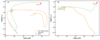 |
Fig. 9. Complete evolutionary tracks for both components in the binary system from the ZAMS through the BLAP phase and their subsequent evolution until the onset of CE. Panel (a): Evolutionary path of the primary star as it transitions from the ZAMS through the BLAP phase (solid orange line) and its subsequent evolution towards the CE phase (dashed green line), with the red triangle marking the point of CE initiation. Panel b: Corresponding evolution of the secondary star, illustrating its evolution until the system enters the CE phase, following the same line style and colour conventions as panel a. |
The binding energy of the MS star was calculated to be −5.43 × 1048 erg. In an extreme scenario of CE ejection, the limiting separation of the two stars is given by  . In contrast, the separation before entering the CE phase is 49 R⊙. As a result, the orbital energy decreases by 7.61 × 1047 erg. Based on these energy values, the calculated αCE is approximately 7.14. The widely accepted range for αCE is approximately 0–1.5. This discrepancy suggests that the orbital energy is likely insufficient to unbind the CE, leading to the conclusion that the two stars will ultimately merge.
4.2. Elemental abundances on the surfaces of the MS
In binary systems experiencing mass transfer, the accretion of material from a donor star onto its companion fundamentally alters the surface abundances of the accreting star. For example, helium enrichment directly indicates mass accretion from a helium-rich donor star. Likewise, enhanced nitrogen abundance relative to carbon and oxygen signals the accretion of CNO-processed material. These elemental signatures are crucial for understanding the history of mass transfer and tracing evolutionary pathways.
Our MESA evolutionary calculations provide quantitative predictions for the photospheric abundances of the B-type MS star. Figure 10 illustrates that our simulations reveal significant enhancements in helium and nitrogen abundances at the surface of the mass-accreting MS star. Specifically, the helium mass fraction reaches XHe = 0.68, while the nitrogen abundance is elevated to XN = 0.01. The derived surface composition exhibits characteristic signatures consistent with the accretion of CNO-processed material originating from an evolved donor. Furthermore, our analysis of the isotopic abundance ratios reveals: 13C/12C = 0.286886, 14N/15N = 23873, 17O/16O = 0.070507, and 18O/16O = 0.000011.
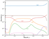 |
Fig. 10. Distribution of elemental abundances in the MS star after mass transfer, with distinct enhancements in 4He and 14N abundances. |
However, the lack of detailed spectroscopic analysis for HD 133729 presents a challenge for directly validating our theoretical models. Future high-resolution spectroscopic studies are crucial for accurately measuring the surface abundances of He and N in the B-type MS star. Confirmation of these abundance anomalies would strongly support the viability of this evolutionary pathway.
4.3. Broader applications of the model
Previous study presents the orbital period and companion mass distribution for stars in the BLAP phase (see Fig. 9 of Byrne et al. 2021). The orbital period exhibits a bimodal distribution, with a minor peak around 1.2 days and a more prominent peak at an orbital period of ∼40 days. Based on the orbital period of HD 133729 and our calculations, we propose that the second peak in the orbital period distribution likely arises from RLOF, while the first peak originates from the CE ejection. Our aim is not only to explain HD 133729 but also to provide a broad grid of calculated parameters.
5. Summary
This study systematically explores the origin and evolution of binary BLAP systems, with a particular focus on HD 133729. We investigated a broad parameter space of mass ratios (q = 0.25, 0.30, 0.35, and 0.45) and initial orbital periods, finding that the pre-WD RLOF channel is the most viable formation pathway for HD 133729. Our simulations show that while a conservative mass transfer model with q = 0.30 reproduces many of the observed properties (orbital period, pulsation period, and rate of period change), it overestimates the effective temperature of the B-type MS star.
To reconcile this discrepancy, we considered non-conservative mass transfer with an isotropic re-emission wind efficiency of β = 0.15, which yielded a better agreement with the observed temperature. The best-fit model for HD 133729 has component masses of M1,i = 2.68 M⊙ and M2,i = 0.78 M⊙, and an initial orbital period of Pi = 3.254 day. Furthermore, we predict that the system will undergo a CE phase during the second mass transfer episode, ultimately leading to a merger.
Our results also highlight the importance of surface abundance evolution. After the first mass transfer phase, we expect notable helium and nitrogen enhancements in the B-type MS companion due to the accretion of CNO-processed material. Such abundance signatures can be directly tested with high-resolution spectroscopy. Furthermore, we have found that non-conservative mass transfer plays a crucial role in the evolution of BLAPs. This provides a novel approach for constraining mass loss during mass transfer in binary systems, potentially offering insights beyond the scope of traditional asteroseismology.
Acknowledgments
We would like to thank Thomas Kupfer, Andrzej Pigulski, and Evan B. Bauer for their help. This study is supported by the National Natural Science Foundation of China (Nos 12288102, 12225304, 12090040/12090043, 12473032, 12473028), the National Key R&D Program of China (No. 2021YFA1600404), the Western Light Project of CAS (No. XBZG-ZDSYS-202117), the science research grant from the China Manned Space Project (No. CMS-CSST-2021-A12), the Yunnan Revitalization Talent support Program (Yunling Scholar Project), the Yunnan Fundamental Research Project (No. 202201BC070003, 202501AS070005), and the International Centre of Supernovae, Yunnan Key Laboratory (No. 202302AN360001). We thank the referee for the helpful suggestions and comments that improved the manuscript.
References
- Borowicz, J., Pietrukowicz, P., Mróz, P., et al. 2023, Acta Astron., 73, 1 [NASA ADS] [Google Scholar]
- Bradshaw, C. W., Dorsch, M., Kupfer, T., et al. 2024, MNRAS, 527, 10239 [Google Scholar]
- Byrne, C. M., & Jeffery, C. S. 2018, MNRAS, 481, 3810 [NASA ADS] [CrossRef] [Google Scholar]
- Byrne, C. M., Stanway, E. R., & Eldridge, J. J. 2021, MNRAS, 507, 621 [NASA ADS] [CrossRef] [Google Scholar]
- Chang, S.-W., Wolf, C., Onken, C. A., & Bessell, M. S. 2024, MNRAS, 529, 1414 [NASA ADS] [CrossRef] [Google Scholar]
- Charpinet, S., Fontaine, G., Brassard, P., & Dorman, B. 1996, ApJ, 471, L103 [Google Scholar]
- Córsico, A. H., Romero, A. D., Althaus, L. G., Pelisoli, I., & Kepler, S. O. 2018, arXiv e-prints [arXiv:1809.07451] [Google Scholar]
- Eddington, A. S. 1918, MNRAS, 79, 2 [NASA ADS] [Google Scholar]
- Grevesse, N., & Sauval, A. J. 1998, Space Sci. Rev., 85, 161 [Google Scholar]
- Hu, H., Tout, C. A., Glebbeek, E., & Dupret, M. A. 2011, MNRAS, 418, 195 [NASA ADS] [CrossRef] [Google Scholar]
- Hurley, J. R., Tout, C. A., & Pols, O. R. 2002, MNRAS, 329, 897 [Google Scholar]
- Jeffery, C. S., & Saio, H. 2016, MNRAS, 458, 1352 [NASA ADS] [CrossRef] [Google Scholar]
- Kołaczek-Szymański, P. A., Pigulski, A., & Łojko, P. 2024, A&A, 691, A103 [NASA ADS] [CrossRef] [EDP Sciences] [Google Scholar]
- Kupfer, T., Bauer, E. B., Burdge, K. B., et al. 2019, ApJ, 878, L35 [Google Scholar]
- Lin, J., Wu, C., Wang, X., et al. 2023, Nat. Astron., 7, 223 [Google Scholar]
- McWhirter, P. R., & Lam, M. C. 2022, MNRAS, 511, 4971 [NASA ADS] [CrossRef] [Google Scholar]
- Meng, X.-C., Han, Z.-W., Podsiadlowski, P., & Li, J. 2020, ApJ, 903, 100 [NASA ADS] [CrossRef] [Google Scholar]
- Neo, S., Miyaji, S., Nomoto, K., & Sugimoto, D. 1977, PASJ, 29, 249 [NASA ADS] [Google Scholar]
- Paczyński, B., & Sienkiewicz, R. 1972, Acta Astron., 22, 73 [NASA ADS] [Google Scholar]
- Paxton, B., Bildsten, L., Dotter, A., et al. 2011, ApJS, 192, 3 [Google Scholar]
- Paxton, B., Cantiello, M., Arras, P., et al. 2013, ApJS, 208, 4 [Google Scholar]
- Paxton, B., Marchant, P., Schwab, J., et al. 2015, ApJS, 220, 15 [Google Scholar]
- Paxton, B., Schwab, J., Bauer, E. B., et al. 2018, ApJS, 234, 34 [NASA ADS] [CrossRef] [Google Scholar]
- Paxton, B., Smolec, R., Schwab, J., et al. 2019, ApJS, 243, 10 [Google Scholar]
- Pietrukowicz, P., Dziembowski, W. A., Mróz, P., et al. 2013, Acta Astron., 63, 379 [Google Scholar]
- Pietrukowicz, P., Dziembowski, W. A., Latour, M., et al. 2017, Nat. Astron., 1, 0166 [Google Scholar]
- Pietrukowicz, P., Latour, M., Soszynski, I., et al. 2024, ApJ, submitted [arXiv:2404.16089] [Google Scholar]
- Pigulski, A., Kotysz, K., & Kołaczek-Szymański, P. A. 2022, A&A, 663, A62 [NASA ADS] [CrossRef] [EDP Sciences] [Google Scholar]
- Pigulski, A., Kołaczek-Szymański, P. A., Święch, M., Łojko, P., & Kowalski, K. J. 2024, A&A, 691, A343 [NASA ADS] [CrossRef] [EDP Sciences] [Google Scholar]
- Ramsay, G., Woudt, P. A., Kupfer, T., et al. 2022, MNRAS, 513, 2215 [NASA ADS] [CrossRef] [Google Scholar]
- Ritter, H. 1988, A&A, 202, 93 [NASA ADS] [Google Scholar]
- Romero, A. D., Córsico, A. H., Althaus, L. G., Pelisoli, I., & Kepler, S. O. 2018, MNRAS, 477, L30 [NASA ADS] [CrossRef] [Google Scholar]
- Schneider, F. R. N., Izzard, R. G., Langer, N., & de Mink, S. E. 2015, ApJ, 805, 20 [Google Scholar]
- Shibahashi, H., Kurtz, D. W., & Murphy, S. J. 2025, arXiv e-prints [arXiv:2502.09444] [Google Scholar]
- Soberman, G. E., Phinney, E. S., & van den Heuvel, E. P. J. 1997, A&A, 327, 620 [NASA ADS] [Google Scholar]
- Wu, T., & Li, Y. 2018, MNRAS, 478, 3871 [NASA ADS] [CrossRef] [Google Scholar]
- Xiong, H., Casagrande, L., Chen, X., et al. 2022, A&A, 668, A112 [NASA ADS] [CrossRef] [EDP Sciences] [Google Scholar]
- Zhang, X., Jeffery, C. S., Su, J., & Bi, S. 2023, ApJ, 959, 24 [NASA ADS] [CrossRef] [Google Scholar]
- Zhang, Z., Wu, C., Aryan, A., et al. 2024, ApJ, 975, 186 [Google Scholar]
All Tables
All Figures
|
Fig. 1. Schematic diagram for the origin of BLAPs. The starting point of the arrow indicates the stellar evolutionary pathway, while the end represents the star’s evolutionary state. |
| In the text | |
|
Fig. 2. Evolution tracks of a binary system consisting of a M1 = 2.72 M⊙ primary and a M2 = 0.68 M⊙ companion. The x-axis shows the model number. Solid lines represent the orbital period (left y-axis) and dashed lines the logarithm of the mass transfer rate (right y-axis). Different colours correspond to initial orbital periods ranging from 1.0 to 4.0 days. |
| In the text | |
|
Fig. 3. Same as Fig. 2 but for a binary system consisting of a M1 = 2.14 M⊙ primary and a M2 = 0.75 M⊙ companion. |
| In the text | |
|
Fig. 4. HR diagram for all RLOF channel models with a mass ratio of 0.35. Different line styles represent different binary masses, and different colours represent different initial orbital periods. |
| In the text | |
|
Fig. 5. Relationship between final and initial orbital periods for binary systems with mass ratio q = 0.30. Polynomial fits are applied to the four datasets. The horizontal dashed black line represents a final orbital period of 23.08 days. |
| In the text | |
|
Fig. 6. Evolutionary tracks on the HR diagram for binary systems with optimal initial orbital periods derived from polynomial fits. Panel a: Evolutionary paths of the primary stars from the ZAMS through the BLAP phase. Panel b: Corresponding evolutionary tracks of the secondary stars. |
| In the text | |
|
Fig. 7. Diagnostic diagrams showing the evolution of stellar parameters for four binary models selected based on their final orbital period. Panel a: Relationship between effective temperature and surface gravity, with horizontal and vertical dashed lines indicating the observational constraints for BLAP (red: log Teff range; dark blue: log(g/cm s−2) = 4.5). Panel b: Correlation between effective temperature and pulsation period. The horizontal and vertical dashed lines mark the observed BLAP temperature range (red) and the target pulsation period of 32.27 minutes (dark blue), respectively. |
| In the text | |
|
Fig. 8. HR diagram showing the influence of β on the evolutionary tracks of both binary components. Panel a: Evolutionary paths of the primary stars for various β values and initial orbital periods, with the pentagram marking the model that best reproduces the observed orbital period of 23.08 days. Panel b: Corresponding evolutionary tracks of the secondary stars. Different colours represent different β values, while different line styles indicate different initial orbital periods. |
| In the text | |
|
Fig. 9. Complete evolutionary tracks for both components in the binary system from the ZAMS through the BLAP phase and their subsequent evolution until the onset of CE. Panel (a): Evolutionary path of the primary star as it transitions from the ZAMS through the BLAP phase (solid orange line) and its subsequent evolution towards the CE phase (dashed green line), with the red triangle marking the point of CE initiation. Panel b: Corresponding evolution of the secondary star, illustrating its evolution until the system enters the CE phase, following the same line style and colour conventions as panel a. |
| In the text | |
|
Fig. 10. Distribution of elemental abundances in the MS star after mass transfer, with distinct enhancements in 4He and 14N abundances. |
| In the text | |
Current usage metrics show cumulative count of Article Views (full-text article views including HTML views, PDF and ePub downloads, according to the available data) and Abstracts Views on Vision4Press platform.
Data correspond to usage on the plateform after 2015. The current usage metrics is available 48-96 hours after online publication and is updated daily on week days.
Initial download of the metrics may take a while.