| Issue |
A&A
Volume 697, May 2025
|
|
|---|---|---|
| Article Number | A200 | |
| Number of page(s) | 9 | |
| Section | Extragalactic astronomy | |
| DOI | https://doi.org/10.1051/0004-6361/202553665 | |
| Published online | 19 May 2025 | |
Search for γ-ray emission from supernova remnants in the Large Magellanic Cloud: A new cluster analysis at energies above 4 GeV
1
Department of Astronomy, University of Geneva, Chemin Pegasi 51, 1290 Versoix, Switzerland
2
INAF/OAS, via Gobetti 101, 40129 Bologna, Italy
3
INAF/IAPS, via del Fosso del Cavaliere 100, I-00113 Roma, Italy
4
INAF/Osservatorio Astronomico di Palermo, Piazza del Parlamento 1, I-90134 Palermo, Italy
5
Dipartimento di Fisica e Chimica E. Segrè, Università di Palermo, Piazza del Parlamento 1, 90134 Palermo, Italy
⋆ Corresponding author: andrea.tramacere@unige.ch
Received:
2
January
2025
Accepted:
21
March
2025
Context. A search for γ-ray emission from supernova remnants (SNRs) in the Large Magellanic Cloud (LMC) based on the detection of concentrations in the arrival direction Fermi-LAT images of photons at energies higher than 10 GeV found significant evidence for nine sources. This analysis was based on data collected in the time window from August 4, 2008, to August 4, 2020 (12 years).
Aims. In the present contribution, we report the results of a new search extended using a 15-year long (up to August 4, 2023) dataset and to a broad energy range (higher than 4 GeV). The longer baseline and the softer energy lower limit are required to further understand the relation between the X-ray and gamma ray SNRs in the LMC and to investigate the completeness of the sample at low luminosities.
Methods. Two different methods of clustering analysis were applied: minimum spanning tree (MST) and a combination of density-based spatial clustering of applications with noise (DBSCAN) and DENsity-based CLUstEring (DENCLUE) algorithms.
Results. We confirm all previous detections and found positive indications for at least eight new clusters with a spatial correspondence with other SNRs, thus increasing the number of candidate remnants in the LMC or detected in the high-energy γ-rays to 16 sources.
Conclusions. This study extends previous analyses of γ-ray emission from SNRs in the LMC by incorporating a longer observational baseline and a broader energy range. The improved dataset and advanced clustering techniques enhance our understanding of the connection between X-ray and γ-ray SNRs, providing new insights into their high-energy properties and contributing to the assessment of the completeness of the sample at lower luminosities.
Key words: methods: data analysis / methods: numerical / methods: statistical / gamma rays: general
© The Authors 2025
 Open Access article, published by EDP Sciences, under the terms of the Creative Commons Attribution License (https://creativecommons.org/licenses/by/4.0), which permits unrestricted use, distribution, and reproduction in any medium, provided the original work is properly cited.
This article is published in open access under the Subscribe to Open model. Subscribe to A&A to support open access publication.
1. Introduction
The Large Magellanic Cloud (LMC) is a nearby irregular galaxy particularly rich with supernova remnants (SNRs), whose ages are in the interval from about 40 years to a few tens of thousands of years. The LMC therefore provides a unique laboratory to investigate high-energy processes related to the interaction of shock waves with interstellar gas and particle acceleration. In particular, these energetic processes can be traced by the detection of γ-ray emission from GeV to TeV energies.
The first observation of the LMC at energies higher than 100 MeV was done by Sreekumar et al. (1992) on the basis of Compton Gamma Ray Observatory (CGRO) EGRET data. Later, Abdo et al. (2010) reported a first study of the LMC using data from the 11-month Fermi-Large Area Telescope (Fermi-LAT; Ackermann et al. 2012) and discovered a bright, extended high-energy source associated with the massive star-forming region 30 Doradus. Ackermann et al. (2016) performed the first detailed analysis of the LMC region by considering much richer Fermi-LAT data spanning the first 6 years of the mission and detected four distinct γ-ray sources. Since then, only a few research papers have been published about the discovery of SNRs in the γ-ray band. The latest version (DR4, v34) of the 4FGL catalog released by the Fermi-LAT collaboration (Abdollahi et al. 2020; Ballet et al. 2020) contains 18 sources detected in the 50 MeV–1 TeV energy range. Of these, four are reported as extended features, and seven are present also in the 3FHL catalog (Ajello et al. 2017) at energies above 10 GeV. Furthermore, possible background extragalactic counterparts (unclassified blazar or BL Lac objects) are indicated for nine of these 4FGL sources.
At TeV energies, the H.E.S.S. collaboration observed three sources up to about 10 TeV in the LMC (H.E.S.S. Collaboration 2015), with two of them being associated with the SNRs N 157B (H.E.S.S. Collaboration 2012) and N 132D. The former contains the highest known spin-down luminosity pulsar, PSR J0537−6910 (Marshall et al. 1998; Cusumano et al. 1998), whose fast period is 16 ms.
Campana et al. (2018b) (hereafter Paper I) used the data collected by the Fermi-LAT telescope in 9 years of operation for a photon cluster search at energies higher than 10 GeV and reported the discovery of high-energy emission from the two SNRs N 49B and N 63A. In a subsequent work (Campana et al. 2022, Paper II), a more complete search was applied to the Fermi-LAT data over 12 years with energy higher than 6 and 10 GeV and using two cluster-finding methods. The detections of Paper I were confirmed, and new significant clusters associated with the SNRs N49 and N44 were found. Furthermore, another cluster likely associated with N186D was detected at energies higher than 6 GeV. The first two sources are among the brightest X-ray remnants in the LMC and correspond to core-collapse (CC) supernovae interacting with dense H II regions, indicating that a hadronic origin of high-energy photons is the favored process. Furthermore, the discovery above 6 GeV of a cluster corresponding to the not-very-bright SNR N186D suggested that other remnants of comparable luminosity can be found when extending the search to lower energies, thus calling for an extension of the analyses in Papers I and II with a longer baseline and a softer energy lower limit.
In the present paper, we extend the analysis of the LMC region using a richer dataset of 15 years of Fermi-LAT observation and energies higher than 4 GeV. As in Paper II, we apply the two cluster-finding methods density-based spatial clustering of applications with noise (DBSCAN) (Tramacere & Vecchio 2013), and the minimum spanning tree (MST; see Campana et al. 2008, 2013 for recent use in γ-ray astronomy) in order to extract photon spatial concentrations likely corresponding to genuine γ-ray sources. The MST method has already been successfully applied in several works (Bernieri et al. 2013; Campana et al. 2015, 2016a,b,c, 2017, 2018a; Campana & Massaro 2021). In the present analysis the DBSCAN algorithm has been coupled to the DENsity-based CLUstEring (DENCLUE) algorithm (Tramacere et al. 2016), in order to handle confused sources.
The results of this new analysis confirm the previous SNR detections with a higher significance. Moreover, some other photon clusters are found at positions very close to those of SNRs not previously associated with γ-ray emitters.
The outline of this paper is as follows. In Sect. 2, the data selection and the MST and DBSCAN and DENCLUE algorithms are described, while the analysis of the LMC region is presented in Sect, 3. The present status of knowledge on the high-energy sources in the LMC, mainly based on the Fermi catalog, is summarized in Sect. 4. In Sect. 5, we deepen the analysis of some interesting SNR counterparts to photon clusters, while in Sect. 6 the results are summarized and discussed.
2. Data selection in the LMC region
We analyzed 15 years of Fermi-LAT data collected from August 4, 2008, to August 4, 2023, including events above 4 GeV. The complete dataset was retrieved as weekly files from the Fermi Science Support Center archive1. The dataset was processed using the Pass 8, release 3, reconstruction algorithm and includes the instrumental responses. The event lists were then filtered by applying the standard selection criteria on data quality and zenith angle (source class events, evclass 128), front and back converting (evtype 3), up to a maximum zenith angle of 90°. Events were then screened for standard good time interval selection. We selected a region 12° ×9° in Galactic coordinates 271° < l < 287° and −38° < b < −29° and approximately centered at the LMC, and the two cluster-finding algorithms were applied. As in Paper I, the size of this region was chosen to include all of the LMC and its near surroundings, but here the extension in longitude is wider than the one used in the previous study to enhance the cluster extraction at low energy because of the higher mean angular distance between photons
Given the condition of a high local diffuse emission in the LMC, the sorting of point-like sources is a quite delicate work, and particular approaches should be adopted. Our basic choice was to search clusters at energies higher than 10 GeV since the diffuse component is rather weak in this band. Once a list of clusters was obtained, we searched for correspondent features at lower energies, and if they were found, the cluster was considered to be confirmed. However, in these analyses, we had to use smaller fields not including the 30 Dor nebula because its relatively high number of photons produces a too short mean angular separation in the field for a safe cluster search. Analyses at lower energies generally imply that the resulting “cluster parameters” (as defined in the following) are generally much lower than above 6 GeV, and the extraction of clusters is less stable. In particular, small changes in the selection parameters could yield different structures.
The LMC is particularly rich in SNRs. The work of Maggi et al. (2016) reports 59 remnants. A richer catalog provided by Bozzetto et al. (2017), which includes the previous one, adds another group of 15 SNR candidates. A further sample of 19 optically selected SNR candidates has been given by Yew et al. (2021). A new complete catalog (hereafter ZMC24) has been recently published by Zangrandi et al. (2024). It is based on the eROSITA X-ray survey and includes 78 entries. As will be clear from the results of this work, we did not find any well-established positional correspondence between clusters and the Yew et al. (2021) sources, the Bozzetto et al. (2017) candidate sources, and the new additions of eROSITA to the list of Maggi et al. (2016). Therefore, we limited our analysis to the last sample, which contains the brightest genuine SNRs.
3. Description of photon cluster detection algorithms
3.1. DBSCAN and DENCLUE
The DBSCAN algorithm is a density-based clustering method that uses the local density of points to find clusters in datasets that are affected by background noise. Here, we give only a brief description of the method and its application (for a detailed description, see Tramacere & Vecchio 2013). We let D be a set of photons where each element is described by the sky coordinates. The distance between two given elements (pl, pk) is defined as the angular distance on the unit sphere, ρ(pl, pk). We let Nε(pi) be the set of points contained within a radius ε, centered on pi, and |Nε(pi)| is the number of contained points, that is, the estimator of the local density, whereas K is the threshold value such that |Nε(pi)| ≥ K defines “core” points. The DBSCAN builds the cluster by recursively connecting “density connected” points to each set of “core” points found in D. Each cluster Cm is described by the position of the centroid (xc, yc), the ellipse of the cluster containment, the number of photons in the cluster (Np), and the significance. The ellipse of the cluster containment is evaluated using the principal component analysis method. The significance of a cluster (Scls) is evaluated according to the signal-to-noise likelihood ratio test (LRT) method proposed by Li & Ma (1983), which is explained in detail in Tramacere & Vecchio (2013) (see also Paper II).
To optimize the clustering process, we needed to set proper values for both ε and K. Thus, we proceeded as follows:
-
We set the radius ε to be half of the instrument point spread function (PSF) at a given threshold energy.
-
We evaluated the initial value of the background density level ηbkg equal to the number of photons within the field divided by the field angular extent, and we set K = NrejηbkgΩε, where Ωε is the solid angle encompassed by the radius ε and Nrej is the background rejection factor, which we set to four, to get a conservative rejection level at a 2σ confidence level.
-
We performed a first DBSCAN detection using the parameters obtained at step 2. We updated the value ηbkg by removing the angular extent of each detected cluster from the field angular extent and the number of corresponding photons, thus obtaining a new value ηbkg*.
-
We performed a second DBSCAN detection, updating K with the updated ηbkg*.
-
We evaluated the significance of each cluster Scls defined as
where Nsrcin is the number of points in each cluster and Nbkgeff is the expected number of background photons within the circle enclosing the most distant cluster point, according to the value of Nbkg estimated from ηbkg*, and then we removed those below the threshold value.
![$$ \begin{aligned} S_{\rm cls}=\sqrt{2 \left( N^\mathrm{in}_{\rm src} \ln \left[ \frac{2 N^\mathrm{in}_{\rm src}}{N^\mathrm{in}_{\rm src}+N^\mathrm{eff}_{\rm bkg}} \right]+ N^\mathrm{eff}_{\rm bkg} \ln \left[ \frac{2N^\mathrm{in}_{\rm src}}{ N^\mathrm{in}_{\rm src}+N^\mathrm{eff}_{\rm bkg}} \right] \right)}, \end{aligned} $$](/articles/aa/full_html/2025/05/aa53665-25/aa53665-25-eq1.gif)
When sources are very close, the DBSCAN algorithm might not be able to separate them. The possibility of blended sources increases when the density of background photons exhibits gradients requiring different values of K across the same sky region. This was not the case in the analysis presented in Paper I, where we used a threshold of 6 GeV, but it became more relevant in the current analysis since we reduced the threshold to 4 GeV. To deblend two (or more) “confused” sources, we used the DENCLUE algorithm (Hinneburg & Keim 1998; Hinneburg & Gabriel 2007). Notably, DENCLUE relies on kernel density estimation, defining clusters according to the local maxima of an estimated density function. This function, f(p), based on a Gaussian kernel in the current application, represents the sums of the “influence” of each point in a dataset, {p1, ..., pj}, on the position p of the data space. A sub-set of points converging to the same local maximum defines a cluster. The identification of the sub-set is accomplished by finding for each point, pj, in the dataset the corresponding “density attractor” point, pj*, that is, a local maximum of f(p). Hence, by clustering the density attractors, each cluster of density attractors, ACn, will identify a common convergence point for the corresponding points {pk : pk* ∈ ACn}; that is, {pk* ∈ ACn} will map a new sub-cluster of points {pk ∈ CDn}. An application of the DENCLUE algorithm for deblending confused sources is given in Tramacere et al. (2016), and a detailed description of this algorithm is reported in Appendix A. The deblending process, applied to each cluster detected by the DBSCAN, proceeded as follows:
-
We set the values of the kernel width h according to the instrument PSF at a given threshold energy.
-
Each cluster, Cm, detected by the DBSCAN defines a set of points {pj ∈ Cm} corresponding to the coordinates of the photons in the cluster and was processed by DENCLUE.
-
All the attractor points, pj*, found in a Cm were clustered using the DBSCAN, providing a list of clusters of density attractors {AC1, ..., ACn} and mapping a corresponding list of deblended sub-clusters, {CD1, ..., CDn}. Of course, if a DBSCAN cluster, Cm, results in a single cluster of attractors, {AC1}, then Cm would not be partitioned in sub-clusters, that is, CDn ≡ {AC1}≡Cm.
-
Each sub-cluster CDn was eventually validated or discarded according to its cluster significance as evaluated in Eq. (1).
3.2. Minimum spanning tree
The MST method is a topometric tool useful for searching for spatial concentrations in a field of points (see, for instance, Cormen et al. 2009 and also Campana et al. 2008, 2013). The application of this method to the γ-ray sky and selection criteria have been presented elsewhere (e.g., in Campana et al. 2018b). We therefore only summarize how the MST parameters were optimized to enhance the detection of photon clusters above 4 GeV in the LMC region.
If one considers a two-dimensional set of Nn points (nodes), there is a unique “tree” (a graph without closed loops) connecting all the nodes with the minimum total weight, min[Σiλi], where the elements of the set {λ} are, in this case, the angular distances between photon arrival directions. The “primary” cluster selection is then performed in two following steps: the elimination of all the edges having a length λ ≥ Λcut, which is convenient to give in units of the mean edge length Λm = (Σiλi)/Nn in the MST, and the removal of all the sub-trees having a number of nodes N ≤ Ncut. This leaves only the clusters with a number of photons higher than this threshold.
For each cluster we evaluated the following parameters: i) the number of nodes in the cluster k, Nk; ii) the clustering parameter gk, defined as the ratio between Λm and λm, k, which is the mean length over the k-th cluster edges; iii) the centroid coordinates, computed by means of a weighted mean of the cluster photon arrival directions (see Campana et al. 2013); iv) the radius of the circle centered at the centroid and containing 50% of the photons in the cluster, which we call the “median radius” Rm (for a genuine point-like γ-ray source, it should be smaller than or comparable to the 68% containment radius of the instrumental PSF); v) the maximum radius Rmax, computed as the distance between the centroid and the farthest photon in the cluster (usually of some arcminutes for a point-like source and a few tens of arcminutes either for extended structures or for unresolved close pairs of sources). A very useful parameter here is the cluster magnitude:

Campana et al. (2013) found that  is well correlated with other statistical source significance parameters, in particular the test significance from the maximum likelihood (Mattox et al. 1996) analysis. The use of these parameters depends on the structure of the sky region under consideration. For example, in fields with a non-high spatial photon density, such as those at energies above 10 GeV, a lower threshold value of M around 15–20 would reject a large majority of the spurious low-significance clusters, while in dense fields M, values lower than 15 can correspond to significant clusters.
4. LMC sources in 4FGL-DR4 catalog
There are 13 sources in the 4FGL-DR4 catalog of the Fermi-LAT collaboration in the region limited by the intervals l ∈ (275, 284) and b ∈ ( − 37, −30) in Galactic coordinates. This region also contains all SNRs of the main catalogs.
Four of the 13 sources are classified as extended. The largest one, 4FGL J0519.9−6845e, has a radius of 3° and essentially includes the most active region of the LMC, as 57 of the ZMC24 sources are within its area. Two of the other extended sources have a radius of 54′ and are contained in the largest one: they are 4FGL J0530.0−6900e, corresponding to the 30 Doradus complex, and 4FGL J0500.9−6945e in the far west region. The former region contains six SNRs and the latter has five. Furthermore, 4FGL J0531.8-6639e, indicated as LMC-North, has the smallest radius at 36′. It contains one SNR and has another one on its edge.
Four of the remaining point sources within this region are associated with blazars or blazar candidates. The source i) 4FGL J0534.1−7218 is the likely counterpart of the BL Lac object 5BZB J0533−7216 (this is the only source not already included in the 4FGL-DR3 version). The source ii) 4FGL J0529.3−7243, corresponding to a CRATES flat-spectrum source, is located in a rather peripheral position and could actually be a background blazar. The source iii) 4FGL J0517.9−6930c, with the final code “c” indicating that it is “confused with interstellar cloud complexes,” is within the area of 4FGL J0519.9−6845e and is located between the two close SNRs N 120 (9 5) and B0520−694 (10
 4). It is associated with the source MC4 0518−696A. The source iv) 4FGL J0535.7−6604c is again classified as a bcu and is associated with the radio source PKS 0535−66, which is not a radio loud active galactic nucleus but it has been safely identified with the counterpart of the SNR N 63A since early observations (Westerlund & Mathewson 1966; Dickel et al. 1993). As mentioned above, we reported a γ-ray cluster corresponding to this source in Paper I, and it was well confirmed by a subsequent analysis in Paper II.
Two other sources, namely 4FGL J0537.8−6909 (P2 in Ackermann et al. 2016) and 4FGL J0524.8−6938 (P4), are associated with the two powerful SNRs N 157B and N 132D, respectively. The source 4FGL J0540.3−6920 (P1) has been securely identified with the young pulsar PSR J0540−6919 Fermi LAT Collaboration (2015). Finally, the two sources 4FGL J0535.2−6736 (P3) and 4FGL J0511.4−6804 are reported without indication for possible counterparts. Corbet et al. (2016) associated the former source with the high-mass X-ray binary (HMXB) CORK053600.0−673507, which according to Seward et al. (2012) appears to be located in the SNR DEM L241.
In addition to these sources, Eagle et al. (2023) reported the detection of a new source in the LMC that was associated with the SNR B0453−685.s which is classified as a pulsar wind nebula (PWN) despite an inner pulsating source has not been detected to now.
5. Results of cluster analysis at energies above 4 and 10 GeV
5.1. Results above 10 GeV
The first step in our analysis was to verify the SNR detections reported in Paper II. It would be expected that the addition of a rather low number of photons (about 25%) does not change the main findings of that analysis. However, it should be taken into account that even a single photon can modify the cluster parameters and move their values across the selection threshold or join two close clusters.
As reported in Table 1, all clusters in Paper II are safely confirmed by both methods. In particular, the DBSCAN/DENCLUE significance was higher than three standard deviations for all sources in the two considered energy ranges, with the exception of the two very close SNRs N 49 and N 49B, which were unresolved, while they are separated by MST. The detection of the SNR N 186D is now confirmed by DBSCAN/DENCLUE at energies higher than 10 GeV, whereas MST analysis gives in this range a cluster with the same number of photons as in Paper II but a slightly lower M due to the higher mean photon density. In the lower energy range, MST finds a cluster of only nine photons and a marginal M value.
Supernova remnants already detected at energies higher than 4 and 10 GeV and confirmed by the present analysis.
5.2. Results above 4 GeV
As explained above, the search for photon clusters above 4 GeV is more difficult because of the large increase of the background and a broader PSF both implying a consequent decrease in the density contrast. As a consequence, the definition of selection thresholds and the significance of clusters cannot be safely established. Therefore, we first applied the DBSCAN/DENCLUE algorithm, whose output gives significance estimates of individual clusters. We then crosschecked these clusters by means of MST. This analysis produced a sample of 35 clusters with a significance higher than three standard deviations. Notably, among these clusters, 12 were already found in Paper II, and seven were found with a close positional correspondence with SNRs, well within the PSF radius at this energy. The properties and the search for counterparts of the remaining 16 clusters will be presented in another paper.
We note that the values of the magnitude M, our main selection parameter defined in Eq.(2), are generally higher than 20, which is the threshold we adopted in the cluster search above 10 GeV. This value can also be adopted at energies higher than 4 GeV, where magnitude values of clusters associated with sources in the 4FGL-DR4 catalog are even lower. As reported in Table 2, only two clusters have an M value lower than 20. One has an M value of 19.8, which is very close to the threshold value, and the other has M = 18.3, which is very much acceptable at these energies.
New SNRs detected at energies higher than 4 GeV.
We also performed a new MST analysis, with Λcut = 0 : 8, in a different region defined by the following boundaries l∈ (274; 281) and b∈ (−40; −33), thus excluding the bright 30 Dor complex. The results of this search confirmed the clusters corresponding to the powerful SNRs with the same numbers of photons but with slightly higher magnitude values above the nominal threshold of 20, namely: M = 20.2 for B0453−685, M = 21.8 for N103B, and M = 29.4 for B0519−690. For comparison, we found two clusters corresponding to non-extended sources in 4FGL-DR4. The cluster associated with 4FGL J0511.4−6804 has 18 photons and M = 43.4, and the one associated with 4FGL J0443.3−6652 has 10 photons and M = 21.2, thus comparable to those of the three remnants indicated above. As further verification of SNR N103B, we analyzed the data at energies higher than 6 GeV and found very close to its position a cluster of only five photons but a quite high clustering parameter of g = 3.2, as defined in Sect. 3.2.
Five clusters were found in the standard analysis over the very large field. The cluster likely associated with [HP99]1139 was found at energies higher than 6 GeV but not above 4 GeV, and the one associated with the complex DEM L316A/B was not found in the very large field, whereas a positive detection resulted in a narrow field excluding the bright region of 30 Dor. We also searched in the primary selection list of clusters above 10 GeV for entries corresponding to these remnants, and we found only a low-significance cluster at the position of DEM L241, whose photon number is the highest. The properties of these two interesting sources are discussed in detail in Sects. 5.3 and 5.4.
In Figure 1, a map of the galaxy is shown with the locations of the clusters. The new ones are outside the very bright region of 30 Dor. In particular, the four clusters associated with faint SNRs are placed at distances greater than 1 degree from the external boundary. The other three clusters in Table 2 (i.e., B0453−685, N 103B, and B0519−690) are in the subsample of bright X-ray emitters undetected in Paper II, and therefore they could be considered as best candidates. In particular, the first of them was already detected by Eagle et al. (2023), while the other two are new findings.
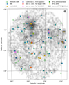 |
Fig. 1. Map of the region of the LMC reporting the known SNRs, 4FGL-DR4 sources, and the photon clusters found in the present work. Solid squares identify SNRs from Maggi et al. (2016). Green empty squares identify SNRs from Zangrandi et al. (2024). Blue diamonds identify confirmed clusters form Campana et al. (2016c), and red and purple diamonds identify clusters detected in the present analysis for bright and faint SNRs, respectively. Yellow crosses mark 4FGL-DR4 point-like sources, dashed circles represent the approximate size of the extended 4FGL sources, the thick circle is that containing the 30 Dor complex, and green stars mark their centers. |
5.3. Properties of the cluster associated with DEM L316A/B
One of the new clusters detected at energies higher than 4 GeV is spatially close to the peculiar object DEM L316A/B, which can be considered a likely counterpart. This source appears to be composed of two overlapping remnants (indicated by the letters A and B) and was investigated in the radio and optical by Williams et al. (1997). However, the possibility that the two remnants are actually interacting has not been confirmed by X-ray data analyses (Williams & Chu 2005; Toledo-Roy et al. 2009). The two remnants are different in size, but both have rather large diameters (2′and 3′, corresponding to about 30 and 40 pc) and are relatively evolved, with estimated ages of 27 kyr and 39 kyr. The centroid coordinates of the cluster given in Table 2 are closer to the remnant A, but it is reasonable that both of these objects can contribute to the photon cluster because Rmax is equal to 6 7 and the angular distance between the centers of the remnants is around 2
 4, thus lower than the instrumental PSF at 4 GeV. The spectra of the two remnants are remarkably different, particularly for the Fe abundance, which indicates that the A shell had a Ia supernova origin, whereas the B originated from a CC supernova (Nishiuchi et al. 2001). Their X-ray luminosities in the Maggi et al. (2016) catalog are remarkably similar.
The γ-ray cluster is not very significant in the MST search in large fields and an acceptable value of M is obtained only when using a narrow field excluding the 30 Dor region. Similar analyses at energies higher than 6 or 10 GeV gave clusters with lower M values below the threshold. Thus, spectrum of this cluster should be very steep or exhibit a rather sharp cutoff just above 4 GeV.
5.4. Properties of the cluster associated with DEM L241
The source P3 in the early paper by Ackermann et al. (2016) was reported as “unassociated” since DEM L241, as well other possible counterparts, were at a distance from the best-fit position of about 11′ at the 2σ limit. However, its spectrum was found to be quite soft, with an estimated photon index equal to 2.8. The corresponding source in the most recent Fermi-LAT catalog, 4FGL J0535.2-6736, is at an angular distance of about 5′ from the remnant, and the counterpart is the HMXB mentioned in Section 4. This association appears safe given that the γ-ray flux exhibits a very significant modulation with a period of 10.3 days, the same as the HMXB (Corbet et al. 2016). An X-ray source was discovered by Seward et al. (2012) inside the remnant in a Chandra image of DEM L241, and spectral data suggest it comprises an O-type star and a neutron star.
In Paper I, a cluster of only four photons above 10 GeV with a low g was found at an angular distance of 2 8 from the remnant. Further analysis at energies higher than 3 GeV showed evidence for a richer cluster, in agreement with the softness of its spectrum. In Paper II, we found that at energies higher than 6 GeV, the cluster MST (83.643, −67.326) was not close enough to the 4FGL-DR4 source for a safe association. At energies higher than 4 GeV, the present analysis provides a very significant cluster either with DBSCAN or DENCLUE and with MST (25 photons, M = 56.67) at a position fully consistent with the known source and the SNR. The search in the primary MST selection sample above 10 GeV gives a poorly significant cluster at (83.8996, −67.5959) with five photons and M = 9.6, which is again consistent with a soft spectral distribution. One can therefore conclude that high-energy photons are mostly emitted by the HMXB rather than the remnant, and consequently this source is not included in the sample of genuine γ-ray loud SNR.
6. Discussion and conclusions
This present analysis exploiting 15 years of Fermi-LAT observations confirms that the LMC region exhibits a significant clumpy structure in the γ-ray emission and has several photon clusters closely associated with SNRs. Our results confirm all previous detections and reveal positive indications for at least eight new clusters with a spatial correspondence with other SNRs, thus increasing the number of LMC candidate or detected remnants in the high-energy γ-rays to 16 sources, one of which was already found to be associated with an X-ray binary in the remnant DEM L241. The number of γ-ray-detected SNRs in the LMC above 4 GeV is now increased to 15 and represents approximately 25% of the Maggi et al. (2016) sample, or 19% of the eROSITA catalog.
The detected clusters provide valuable insights into the interplay between the intrinsic properties of SNRs and their γ-ray emission. A clear trend emerged that links higher X-ray luminosity in the 0.3 − 8 keV band (LX > 1036 erg s−1; a general indicator of the power output of a SNR) with a higher probability of γ-ray detection. Among the 12 brightest SNRs detected in X-rays, nine are present in our γ-ray cluster list. This correlation underscores the role of the environment, where shock interaction with dense interstellar material and particle acceleration processes produce detectable γ-ray signatures. The remaining six detected SNRs have X-ray luminosities in the range 0.5 − 4.7 × 1035 erg s−1, which is similar to other sources in the sample.
However, some challenges remain. (i) Three SNRs in the bright subsample (B0509−67.5, DEM L71, and N 23) are not associated with significant γ-ray clusters despite expectations of detectable emission. (ii) Six low-luminosity SNRs are detected in γ-rays with different degrees of significance, while several other sources of comparable luminosity remain undetected.
Concerning the first point, the properties of the three remnants suggest plausible explanations for their lack of γ-ray detection. Both B0509−67.5 and DEM L71 exhibit low cosmic-ray acceleration efficiencies. The remnant DEM L71 exhibits enhanced Fe emission and is classified as a Type Ia SNR; its age is estimated to be approximately 6700 years (Frank et al. 2019; Alan & Bilir 2022). According to Rakowski et al. (2003) and Ghavamian et al. (2003), the absence of a non-thermal X-ray component and the low radio flux suggest that the blast wave energy loss to cosmic-ray acceleration is minimal at the current epoch, reducing the probability of detecting high-energy γ-ray emission. The remnant B0509−67.5, on the other hand, is a very young Type Ia SNR originating from an explosion about 400 years ago (Yamaguchi et al. 2014; Kosenko et al. 2014). Based on optical spectroscopic studies, Hovey et al. (2018) determined that this SNR also has a low efficiency for cosmic-ray acceleration. This inefficiency likely explains its lack of significant γ-ray emission despite its young age and high-energy potential. From these observational findings, we conclude that the low cosmic-ray acceleration efficiencies of these remnants can be responsible for their weak or absent high-energy γ-ray signatures.
The case of N 23 is more complex. This object is classified as a CC SNR and contains a candidate PWN identified as the point-like X-ray source CXOU J050552.3−680141 (Hayato et al. 2006). Despite its classification and the potential PWN contribution, N 23 exhibits only faint nebular X-ray emission, and its γ-ray emission remains undetected. This suggests that other factors, such as the properties of the surrounding medium or a lack of sufficient particle acceleration mechanisms, could be suppressing its high-energy output. Further multi-wavelength studies, particularly in the radio and X-ray bands, are needed to clarify the mechanisms limiting γ-ray production in N 23.
Interestingly, these three SNRs are located in a relatively compact region of the LMC, distinct from the high-activity 30 Dor region. The angular separation between DEM L71 and N 23 is only 9′.2, corresponding to a projected distance of approximately 134 pc, while B0509−67.5 lies about 37′ away, or ∼540 pc. This spatial clustering raises the possibility of a shared local environment or regional conditions affecting their γ-ray emission, which merits further exploration.
For what concerns the low-luminosity SNRs associated with γ-ray clusters, the disparity in γ-ray detection between these six remnants and the remaining low-luminosity SNRs of the sample may stem from environmental or intrinsic factors. These include variations in shock efficiency, differences in the density and structure of the surrounding medium, or the strength and configuration of magnetic fields. Such factors significantly affect the ability of remnants to accelerate particles to relativistic energies and produce detectable γ-ray emission. Further investigation is essential to clarify why only six out of about 40 remnants in this category exhibit detectable γ-ray emission. Finding the answer could potentially shed light on the mechanisms driving their high-energy output.
The properties of three of these six SNRs were already discussed in Paper II. N 44 is a complex nebular system that includes three components, one of which is the SNR 0523−679. The source B0528−692, now confirmed as an SNR through our new analysis, shows increased significance and a reduced angular distance between the cluster centroid and the SNR coordinates. However, its position within the brightest region of the LMC raises the possibility of contamination from nearby sources. For the third remnant, N 186D, the photon count remains consistent with Paper II, but its lower M-value results in no significant improvement in detection confidence. Despite this, the association between the cluster and this remnant remains robust.
Three low-luminosity SNRs are detected above 4 GeV. The case of one, DEM L316A/B, is discussed in Sect. 5.3, while literature data on the other two remnants are rather poor. An X-ray image, showing a central bright emission, and a spectral analysis of [HP99]1139 was reported by Whelan et al. (2014), who classified it as Ia type with an age around 19 kyr and a large size, which makes it one of the most extended remnants in the LMC. The detection of a middle-aged SNR below 10 GeV is somehow in line with what happens in our Galaxy, where evolved SNRs are typically characterized by a soft (likely hadronic) γ-ray emission barely extending beyond 10 GeV, while the spectral energy distribution of younger SNRs peaks at higher energies (e.g., Funk 2015). B0532−675 has been investigated by Li et al. (2022), who did not observe an optical shell pattern, but its extension can be derived from the non-thermal radio emission. The OB association LH75 (NGC 2011) is projected within the remnant boundaries, and prevoius authors propose that the supernova progenitor was a star of about 15 solar masses in this association and exploded in an HI cavity. The presence of an OB association might provide a possibility to enhance high-energy emission as proposed by Kavanagh et al. (2019) and Aharonian et al. (2024) for TeV sources detected in the LMC, but in our case this requires more focused studies.
The results of our new cluster analyses of the photon field of the LMC region at TeV energies observed by the Fermi-LAT experiment during 15 years can be summarized as follows:
-
We detected photon clusters whose centroids are at angular separations of only a few arcminutes from 15 SNRs. More specifically, eight SNRs were found above 10 GeV and one above 6 GeV. The other six remnants are above 4 GeV.
-
One of these clusters corresponds to a very close pair of SNRs (DEM L316A and DEM L316B) that have a separation smaller than the PSF diameter, and therefore their γ-ray emission cannot be resolved.
-
There is robust evidence for a cluster corresponding to the SNR DEM L241, a source already detected and exhibiting a clear modulation with the period of an X-ray binary inside the remnant.
-
We also searched for clusters close to the position of the very young SNR 1987A but did not find any significant feature. We recall, however, that this source is close to the bright region of 30 Dor, and the local high spatial density of photons makes cluster extraction quite difficult.
-
The remnants previously reported in Paper II were all of the CC type, while in the present analysis we also found two Ia SNRs, although only at energies higher than 4 GeV. Their emission, therefore, appears generally softer than CC remnants. It is important to verify this trend with other sources, but such investigations require a much longer exposure to achieve sufficient photon statistics.
Given its proximity and particularly the low metallicity and intense star formation history, the LMC provides a unique laboratory with conditions similar to those of primeval galaxies in the early Universe. Our findings are therefore useful to help refine the understanding of young SNR evolution, particle acceleration, and progenitor-type differences, and they also emphasize the need for deeper high-energy observations to verify spectral trends and detect faint sources.
Acknowledgments
F.B., M.M., and S.O. acknowledge financial contribution from the PRIN 2022 (20224MNC5A) – “Life, death and after-death of massive stars” funded by European Union – Next Generation EU, and the INAF Theory Grant “Supernova remnants as probes for the structure and mass-loss history of the progenitor systems”.
References
- Abdo, A. A., Ackermann, M., Ajello, M., et al. 2010, A&A, 512, A7 [NASA ADS] [CrossRef] [EDP Sciences] [Google Scholar]
- Abdollahi, S., Acero, F., Ackermann, M., et al. 2020, ApJS, 247, 33 [Google Scholar]
- Ackermann, M., Ajello, M., Albert, A., et al. 2012, ApJS, 203, 4 [Google Scholar]
- Ackermann, M., Albert, A., Atwood, W. B., et al. 2016, A&A, 586, A71 [NASA ADS] [CrossRef] [EDP Sciences] [Google Scholar]
- Aharonian, F., Benkhali, F. A., Aschersleben, J., et al. 2024, ApJ, 970, L21 [Google Scholar]
- Ajello, M., Atwood, W. B., Baldini, L., et al. 2017, ApJS, 232, 18 [Google Scholar]
- Alan, N., & Bilir, S. 2022, MNRAS, 511, 5018 [Google Scholar]
- Ballet, J., Burnett, T. H., Digel, S. W., & Lott, B. 2020, arXiv e-prints [arXiv:2005.11208] [Google Scholar]
- Bernieri, E., Campana, R., Massaro, E., Paggi, A., & Tramacere, A. 2013, A&A, 551, L5 [EDP Sciences] [Google Scholar]
- Bozzetto, L. M., Filipović, M. D., Vukotić, B., et al. 2017, ApJS, 230, 2 [NASA ADS] [CrossRef] [Google Scholar]
- Campana, R., & Massaro, E. 2021, A&A, 652, A6 [Google Scholar]
- Campana, R., Massaro, E., Gasparrini, D., Cutini, S., & Tramacere, A. 2008, MNRAS, 383, 1166 [Google Scholar]
- Campana, R., Bernieri, E., Massaro, E., Tinebra, F., & Tosti, G. 2013, Ap&SS, 347, 169 [Google Scholar]
- Campana, R., Massaro, E., Bernieri, E., & D’Amato, Q. 2015, Ap&SS, 360, 19 [Google Scholar]
- Campana, R., Massaro, E., & Bernieri, E. 2016a, Ap&SS, 361, 367 [Google Scholar]
- Campana, R., Massaro, E., & Bernieri, E. 2016b, Ap&SS, 361, 185 [Google Scholar]
- Campana, R., Massaro, E., & Bernieri, E. 2016c, Ap&SS, 361, 183 [Google Scholar]
- Campana, R., Maselli, A., Bernieri, E., & Massaro, E. 2017, MNRAS, 465, 2784 [Google Scholar]
- Campana, R., Massaro, E., & Bernieri, E. 2018a, A&A, 619, A23 [NASA ADS] [CrossRef] [EDP Sciences] [Google Scholar]
- Campana, R., Massaro, E., & Bernieri, E. 2018b, Ap&SS, 363, 144 [Google Scholar]
- Campana, R., Massaro, E., Bocchino, F., et al. 2022, MNRAS, 515, 1676 [Google Scholar]
- Corbet, R. H. D., Chomiuk, L., Coe, M. J., et al. 2016, ApJ, 829, 105 [Google Scholar]
- Cormen, T., Leiserson, C., Rivest, R., & Stein, C. 2009, Introduction to Algorithms, 3rd edn. (Cambridge, USA: MIT Press) [Google Scholar]
- Cusumano, G., Maccarone, M. C., Mineo, T., et al. 1998, A&A, 333, L55 [NASA ADS] [Google Scholar]
- Dickel, J. R., Milne, D. K., Junkes, N., & Klein, U. 1993, A&A, 275, 265 [NASA ADS] [Google Scholar]
- Eagle, J., Castro, D., Mahhov, P., et al. 2023, ApJ, 945, 4 [Google Scholar]
- Fermi LAT Collaboration (Ackermann, M., et al.) 2015, Science, 350, 801 [Google Scholar]
- Frank, K. A., Dwarkadas, V., Panfichi, A., Crum, R. M., & Burrows, D. N. 2019, ApJ, 875, 14 [Google Scholar]
- Funk, S. 2015, Ann. Rev. Nucl. Part. Sci., 65, 245 [Google Scholar]
- Ghavamian, P., Rakowski, C. E., Hughes, J. P., & Williams, T. B. 2003, ApJ, 590, 833 [Google Scholar]
- H.E.S.S. Collaboration (Abramowski, A., et al.) 2012, A&A, 545, L2 [NASA ADS] [CrossRef] [EDP Sciences] [Google Scholar]
- H.E.S.S. Collaboration (Abramowski, A., et al.) 2015, Science, 347, 406 [NASA ADS] [CrossRef] [Google Scholar]
- Hayato, A., Bamba, A., Tamagawa, T., & Kawabata, K. 2006, ApJ, 653, 280 [Google Scholar]
- Hinneburg, A., & Gabriel, H.-H. 2007, in Proceedings of the 7th International Conference on Intelligent Data Analysis, IDA’07 (Berlin, Heidelberg: Springer-Verlag), 70 [Google Scholar]
- Hinneburg, A., & Keim, D. A. 1998, in Proceedings of the Fourth International Conference on Knowledge Discovery and Data Mining, KDD’98 (AAAI Press), 58 [Google Scholar]
- Hovey, L., Hughes, J. P., McCully, C., Pandya, V., & Eriksen, K. 2018, ApJ, 862, 148 [Google Scholar]
- Kavanagh, P. J., Vink, J., Sasaki, M., et al. 2019, A&A, 621, A138 [NASA ADS] [CrossRef] [EDP Sciences] [Google Scholar]
- Kosenko, D., Ferrand, G., & Decourchelle, A. 2014, MNRAS, 443, 1390 [Google Scholar]
- Li, T. P., & Ma, Y. Q. 1983, ApJ, 272, 317 [CrossRef] [Google Scholar]
- Li, C.-J., Chu, Y.-H., Chuang, C.-Y., & Li, G.-H. 2022, AJ, 163, 30 [Google Scholar]
- Maggi, P., Haberl, F., Kavanagh, P. J., et al. 2016, A&A, 585, A162 [NASA ADS] [CrossRef] [EDP Sciences] [Google Scholar]
- Marshall, F. E., Gotthelf, E. V., Zhang, W., Middleditch, J., & Wang, Q. D. 1998, ApJ, 499, L179 [Google Scholar]
- Mattox, J. R., Bertsch, D. L., Chiang, J., et al. 1996, ApJ, 461, 396 [Google Scholar]
- Nishiuchi, M., Yokogawa, J., Koyama, K., & Hughes, J. P. 2001, PASJ, 53, 99 [Google Scholar]
- Rakowski, C. E., Ghavamian, P., & Hughes, J. P. 2003, ApJ, 590, 846 [Google Scholar]
- Seward, F. D., Charles, P. A., Foster, D. L., et al. 2012, ApJ, 759, 123 [Google Scholar]
- Sreekumar, P., Bertsch, D. L., Dingus, B. L., et al. 1992, ApJ, 400, L67 [NASA ADS] [CrossRef] [Google Scholar]
- Toledo-Roy, J. C., Velázquez, P. F., de Colle, F., et al. 2009, MNRAS, 395, 351 [Google Scholar]
- Tramacere, A., & Vecchio, C. 2013, A&A, 549, A138 [NASA ADS] [CrossRef] [EDP Sciences] [Google Scholar]
- Tramacere, A., Paraficz, D., Dubath, P., Kneib, J. P., & Courbin, F. 2016, MNRAS, 463, 2939 [Google Scholar]
- Westerlund, B. E., & Mathewson, D. S., 1966, MNRAS, 131, 371 [Google Scholar]
- Whelan, E., Kavanagh, P., Sasaki, M., et al. 2014, in The X-ray Universe 2014, ed. J. U. Ness, 333 [Google Scholar]
- Williams, R. M., & Chu, Y. H. 2005, ApJ, 635, 1077 [Google Scholar]
- Williams, R. M., Chu, Y.-H., Dickel, J. R., et al. 1997, ApJ, 480, 618 [Google Scholar]
- Yamaguchi, H., Badenes, C., Petre, R., et al. 2014, ApJ, 785, L27 [NASA ADS] [CrossRef] [Google Scholar]
- Yew, M., Filipović, M. D., Stupar, M., et al. 2021, MNRAS, 500, 2336 [Google Scholar]
- Zangrandi, F., Jurk, K., Sasaki, M., et al. 2024, A&A, 692, A237 [NASA ADS] [CrossRef] [EDP Sciences] [Google Scholar]
Appendix A: DENCLUE
The DENCLUE algorithm relies on the localization of local maxima in datasets, using a kernel density estimator. Assume that we have a set of instances in a given data space, D = {p1, ..,pn}, and each instance pj ∈ D is a point whose coordinates are represented by the vector qj, with dimensionality d = 2, then the probability density function at a position p in the data space, f(p), can be expressed in terms of a kernel function G as
where h is the kernel bandwidth. The function G represents the influence of the point pi ∈ D with coordinates qi at the position p with coordinates p, hence, the probability density function represents the sum of the influence of all the data points on the point p. The DENCLUE algorithm is designed to find for each point pj ∈ D the corresponding density attractor point pj*, that is, a local maximum of f. To find the attractors, rather than using a computationally expensive gradient ascent approach, we use the fast hill climbing technique presented in int Hinneburg & Gabriel (2007) that is an iterative update rule with the formula:
where the t is the current iteration, t + 1 the updated value, and q(t = 0) ≡ qj represent the coordinate vector of the point pj. The fast hill-climbing starts at each point with coordinate vector qj, and iterates until ∥q(t) − q(t + 1)∥≤εd. The coordinate vector q(t + 1) identifies the position of the density attractorpj* for the point pj. All the attractor points are then clustered using the DBSCAN algorithm, to eventually deblend the confused sources, in a way that can be summarized by the following steps:
-
each cluster Cm, detected by the DBSCAN, is defined by a set of points {pj ∈ Cm}, corresponding to the coordinates of the photons in the cluster
-
for each point pj ∈ Cm we compute the density attractor. It means that ∀pj ∈ Cm, ∃pm*, i.e. the two sets {pm} and {pm*}, map biunivocally Ccls to Cm*.
-
all the attractors points in Cm* are clustered using the DBSCAN, in clusters of density attractors producing a list of clusters of attractors {CA1, ..., CAn}.
-
The set of points pj whose density attractors belong to the same cluster of attractors ACn, i.e. {pj : pj* ∈ CAn}, defines a new sub-cluster CDn
All Tables
Supernova remnants already detected at energies higher than 4 and 10 GeV and confirmed by the present analysis.
All Figures
|
Fig. 1. Map of the region of the LMC reporting the known SNRs, 4FGL-DR4 sources, and the photon clusters found in the present work. Solid squares identify SNRs from Maggi et al. (2016). Green empty squares identify SNRs from Zangrandi et al. (2024). Blue diamonds identify confirmed clusters form Campana et al. (2016c), and red and purple diamonds identify clusters detected in the present analysis for bright and faint SNRs, respectively. Yellow crosses mark 4FGL-DR4 point-like sources, dashed circles represent the approximate size of the extended 4FGL sources, the thick circle is that containing the 30 Dor complex, and green stars mark their centers. |
| In the text | |
Current usage metrics show cumulative count of Article Views (full-text article views including HTML views, PDF and ePub downloads, according to the available data) and Abstracts Views on Vision4Press platform.
Data correspond to usage on the plateform after 2015. The current usage metrics is available 48-96 hours after online publication and is updated daily on week days.
Initial download of the metrics may take a while.