| Issue |
A&A
Volume 697, May 2025
|
|
|---|---|---|
| Article Number | A26 | |
| Number of page(s) | 13 | |
| Section | Planets, planetary systems, and small bodies | |
| DOI | https://doi.org/10.1051/0004-6361/202452842 | |
| Published online | 05 May 2025 | |
Cosmic ray ionisation of a post-impact early Earth atmosphere
Solar cosmic ray ionisation must be considered in origin-of-life scenarios
1
Astronomy & Astrophysics Section, School of Cosmic Physics, Dublin Institute for Advanced Studies,
31 Fitzwilliam Place,
Dublin
D02 XF86,
Ireland
2
School of Physics, Trinity College Dublin, The University of Dublin, College Green,
Dublin 2,
Ireland
3
Cavendish Laboratory, University of Cambridge,
JJ Thomson Ave,
Cambridge
CB3 0HE,
UK
★ Corresponding author; shaunarose@cp.dias.ie
Received:
1
November
2024
Accepted:
2
April
2025
Context. Cosmic rays, both solar and Galactic, have an ionising effect on the Earth’s atmosphere and are thought to be important in the production of prebiotic molecules. In particular, the H2-dominated atmosphere that follows an ocean-vaporising impact is considered favourable to prebiotic molecule formation. As a first step in determining the role that cosmic rays might have played in the origin of life, we need to understand the significance of their ionising effect.
Aims. We model the transport of solar and Galactic cosmic rays through a post-impact early Earth atmosphere at 200 Myr. We aim to identify the differences in the resulting ionisation rates – particularly at the Earth’s surface during a period when the Sun was very active.
Methods. We used a Monte Carlo model for describing cosmic ray transport through the early Earth atmosphere, giving the cosmic ray spectra as a function of atmospheric height. Using these spectra, we calculated the ionisation and ion-pair production rates as a function of height due to Galactic and solar cosmic rays. The Galactic and solar cosmic ray spectra are both affected by the Sun’s rotation rate, Ω, because the solar wind velocity and magnetic field strength both depend on Ω and influence cosmic ray transport. We considered a range of input spectra resulting from the range of possible rotation rates of the young Sun – from 3.5–15Ω⊙. To account for the possibility that the Galactic cosmic ray spectrum outside the Solar System is not constant over gigayear timescales, we compared the ionisation rate at the top of the Earth’s atmosphere resulting from two different scenarios. We also considered the suppression of the cosmic ray spectra by a planetary magnetic field.
Results. We find that the ionisation and ion-pair production rates due to cosmic rays are dominated by solar cosmic rays in the early Earth atmosphere for most cases. The corresponding ionisation rate at the surface of the early Earth ranges from 5 × 10⁻²¹ s−1 for Ω = 3.5Ω⊙ to 1 × 10⁻¹⁶ s−1 for Ω = 15Ω⊙. Thus if the young Sun was a fast rotator (Ω = 15Ω⊙), it is likely that solar cosmic rays had a significant effect on the chemistry at the Earth’s surface at the time when life is likely to have formed.
Conclusions. Cosmic rays, particularly solar cosmic rays, are a source of ionisation that should be taken into account in chemical modelling of the post-impact early Earth atmosphere. Modelling of cosmic ray transport and effects on chemistry will also be of interest for the characterisation of H2-dominated exoplanet atmospheres.
Key words: methods: numerical / Sun: particle emission / Earth / planets and satellites: atmospheres / cosmic rays
© The Authors 2025
 Open Access article, published by EDP Sciences, under the terms of the Creative Commons Attribution License (https://creativecommons.org/licenses/by/4.0), which permits unrestricted use, distribution, and reproduction in any medium, provided the original work is properly cited.
This article is published in open access under the Subscribe to Open model. Subscribe to A&A to support open access publication.
1 Introduction
The origin of life depends on many factors including the presence of a number of key molecules, such as hydrogen cyanide (HCN) and formaldehyde (HCHO), that act as ‘building blocks’ for life and are known as prebiotic molecules (Gargaud et al. 2013; Benner et al. 2020). Cosmic rays – energetic charged particles – are thought to be important in creating the conditions necessary to form these prebiotic molecules in a planetary atmosphere (e.g. Airapetian et al. 2016).
Solar cosmic rays (i.e. particles accelerated by flares and in coronal mass ejections, also known as solar energetic particles) and Galactic cosmic rays, which are collectively referred to as ‘cosmic rays’ throughout, contribute to ionisation in the Earth’s atmosphere (e.g. Sinnhuber et al. 2012). If the rate of cosmic rays impacting the atmosphere is large enough, this ionisation will significantly alter the chemical species present.
Molecules such as HCN (Benner et al. 2019) are described as prebiotic molecules because they are needed to produce the amino acids and RNA bases that go on to form cells – the basic unit of life (Gargaud et al. 2013). The production of many of these molecules appears to require an oxygen-poor environment (Benner et al. 2019). Experiments such as those described in Miller & Schlesinger (1983) highlight the need for an oxygenpoor atmosphere with large amounts of molecular hydrogen (H2). Zahnle et al. (2020) describe how a transient oxygen-poor, H2-rich atmosphere could have been produced on Earth as a result of a large impact early in Earth’s lifetime. Zahnle et al. (2020) present this post-impact early Earth atmosphere scenario as an explanation for the observed excess of metals in the Earth’s mantle which are typically dissolved in iron and would otherwise be expected to be in the core. A single impactor large enough to deliver all of the excess of these metals would be comparable in size (~2300 km diameter) to Pluto (Zahnle et al. 2020). An impact of this size would likely melt and ‘reset’ the crystals used for radiogenic dating of rock in Earth’s crust (Benner et al. 2020). The existence of material in the Earth’s crust which has been dated to >4.35 Gyr ago implies that the transient post-impact atmosphere would have been present when Earth was only a few hundreds of millions of years old (Brasser et al. 2016; Benner et al. 2020).
The properties of the young Sun produce differences in the intensity and energy of cosmic rays reaching Earth compared with the present day. From photometric observations of Sun-like stars (Gallet & Bouvier 2013), which show faster rotation rates at younger ages, we can assume that the Sun’s rotation rate was faster at earlier epochs than at present. The observed scaling of the large-scale magnetic field strength with the rotation rate of low-mass stars (Vidotto et al. 2014) indicates that the young Sun also had a stronger magnetic field than today. This stronger magnetic field and the increased flaring rates of fast rotating lowmass stars (Günther et al. 2020) lead to increased acceleration of solar cosmic rays (Rodgers-Lee et al. 2021) and likely increased the suppression of Galactic cosmic rays by the solar wind at earlier ages (Rodgers-Lee et al. 2020).
Some of the first origin of life studies investigated possible energy sources leading to the synthesis of prebiotic molecules. Miller & Urey (1959) designed experiments to simulate early Earth atmospheres and investigate the efficacy of lightning and solar UV radiation as energy sources for amino acid production. Miller & Urey (1959) suggested that Galactic cosmic rays were unlikely to have a large effect on the atmosphere’s chemistry because the cosmic ray energy density was likely to be negligible in the past. However, they did not consider solar cosmic rays, which are likely to have been present at Earth in greater numbers in the past. More recent experiments (Kobayashi et al. 2023) revisit the question of cosmic rays’ role in forming prebiotic molecules in an early Earth atmosphere, taking into account both Galactic and solar cosmic rays. The results of these experiments point toward solar cosmic rays as the most promising energy sources for prebiotic molecule production.
More broadly, since it is not possible to observe the early Earth atmosphere, spectroscopic observations of exoplanets with different atmospheres in a variety of cosmic ray environments can provide insight into the conditions which promote the production of prebiotic molecules (Rimmer 2023). Cosmic rays can also negatively impact on the likelihood of life on exoplanets – Herbst et al. (2024) model the effect of cosmic rays on Earth-like exoplanet atmospheres, finding that cosmic rays can destroy biosignature molecules, such as ozone, which suggest the presence of life. Rodgers-Lee et al. (2023) model cosmic ray transport in the atmosphere of GJ436b, an exoplanet with an atmosphere comparable to the early Earth which was observed with NIRCam in JWST Cycle 1. Transmission spectroscopy observations of such exoplanets will improve our understanding of origin-of-life scenarios.
Rimmer & Helling (2013) found that cosmic ray ionisation is important to consider in chemical modelling of brown dwarf and free-floating exoplanet atmospheres. Rimmer & Helling (2016) model cosmic ray transport through exoplanet atmospheres including a hydrogen-dominated gas giant. Chemical models such as that presented in Rimmer & Helling (2016) use the cosmic ray ionisation rate as an important input for modelling atmospheric chemistry, including prebiotic molecule production. As a starting point, Rimmer & Helling (2016) use the same top-of-atmosphere cosmic ray spectra for each scenario. Here, our cosmic ray spectra depend on the solar rotation rate and reflect the effects of transport through the solar wind on the spectra. Rodgers-Lee et al. (2021) investigate the cosmic ray intensity at the top of the Earth’s atmosphere at an age of 600 Myr.
Here, we investigate the transport and ionising effect of cosmic rays through the Earth’s atmosphere at 200 Myr, when the oxygen-poor atmosphere required for prebiotic chemistry is thought to have been present. We consider two different scenarios for the Galactic cosmic ray spectrum outside the Solar System which may not be constant on gigayear timescales. We also modify our cosmic ray spectra for the post-impact early Earth atmosphere to account for deflection by a planetary magnetic field. The paper is structured as follows: Section 2 introduces the models that are used for the cosmic ray transport and in Section 3 our results are presented. The discussion and conclusions are given in Sections 4 and 5.
2 Methodology
Here we describe how we have modelled the cosmic ray transport through the early Earth’s atmosphere. Section 2.1 presents the model properties of the atmosphere. Section 2.2 presents the solar wind properties for the early Earth scenario. Section 2.3 details the role of the solar wind in determining the cosmic ray spectra reaching the top of the atmosphere, which are then presented in Section 2.4. Section 2.5 introduces the model used for cosmic ray transport.
2.1 Post-impact early Earth atmosphere model
In this paper, we consider the early Earth’s atmosphere at 200 Myr, after the impact of a Pluto-sized dwarf planet rich in iron. In this scenario, the impactor vaporises the Earth’s oceans, based on the ‘maximum late veneer’ scenario described in Zahnle et al. (2020). The water from the vaporised oceans reacts with the iron from the impactor, producing H2 and FeO through the reaction Fe + H2O → H2 + FeO. The resulting atmosphere is hydrogen-dominated and has a significantly higher pressure at the surface than the present-day, ranging from several tens of bars (Zahnle et al. 2020) to ~120 bar (Itcovitz et al. 2022). We use the terms ‘post-impact early Earth’ and ‘early Earth’ interchangeably to refer to this scenario, except where stated otherwise.
The temperature-pressure profile we used for the post-impact early Earth atmosphere is shown in Fig. 1. This temperature-pressure profile was produced by extrapolating the model temperature-pressure profile of Earth’s atmosphere at ~800 Myr (Fig. 1 from Tian et al. 2011) to a pressure, P = 100 bar. The temperature at the surface is higher than at the present day, exceeding 500 K. The scale height of the atmosphere, H, is calculated as H = kBTatm/gμmp, where Tatm is the atmosphere temperature, g is acceleration due to gravity, μ is the atmosphere’s mean molecular weight and mp is the mass of a proton. For simplicity in our cosmic ray transport simulations we assumed that the atmosphere is 100% H2. Using μ = 2 and assuming a representative Tatm = 530K and constant g, then H = 210 km for the post-impact early Earth atmosphere. For comparison, for Earth’s present-day atmosphere H = 8 km. In Fig. 1, the dashed line represents the temperature-pressure profile for present-day Earth (A. M. Taylor, priv. comm.). For the present-day Earth, the temperature increases with increasing altitude for P < 10−6 bar due to absorption of short-wavelength radiation by N2 and O2, and for 10−3 < P < 10−1 bar due to absorption of solar UV radiation by O3. This level of complexity is not included in our model at present.
Using the ideal gas law, we calculated the number density, n, throughout the atmosphere. The solid line in Fig. 2 shows n as a function of P for the post-impact early Earth atmosphere. The present-day density profile is shown for comparison by the dashed line, showing the difference in number density at the surface (1 bar for the present day Earth, 100 bar for the early Earth) of ~2 orders of magnitude. By assuming hydrostatic equilibrium (dP/dz = −gμmpn), we calculated the height, z, corresponding to each P. The pressure-altitude profile for the early Earth is shown in Fig. A.1. The density profile uses a logarithmically spaced z grid with 250 points. The early Earth atmosphere density profile is required for the cosmic ray transport model, discussed further in Section 2.5.
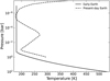 |
Fig. 1 Temperature-pressure profile for a post-impact early Earth atmosphere, with the present-day temperature-pressure profile for comparison. See Section 2.1 for details. |
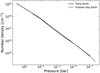 |
Fig. 2 Number density of the atmosphere at 200 Myr (solid line) as a function of pressure, calculated using the ideal gas law and adopted temperature-pressure profile for comparison. The number density for the present-day Earth is shown with the dashed line. |
2.2 Solar wind properties
The motion of cosmic rays in the Solar System is affected by cosmic ray interactions with the magnetised solar wind. The solar wind properties which influence cosmic ray transport in the Solar System (e.g. the diffusion coefficient calculated using the solar wind magnetic field strength, B(r), and radial velocity, vr(r)~v(r)) vary with Ω. For the Sun at 200 Myr, Ω is unknown. At an age of ~200 Myr, for low-mass stars (with M = 0.25–1.1 M⊙) in young clusters the observed rotation rates from photometric observations of stellar surface spots range from 1–100Ω⊙ (Gallet & Bouvier 2013).
Johnstone et al. (2021) fit a rotational evolution model to stellar rotation period measurements for M = 0.9–1.1 M⊙. Johnstone et al. (2021) present rotational evolution tracks for slow, medium, and fast rotator cases fit to the 5th (Ω = 3.5Ω⊙), 50th (Ω = 6 Ω⊙), and 95th (Ω = 15Ω⊙) percentile of the Ω measurements, respectively. We used these three different possible rotation rates for the Sun at 200 Myr and modelled the subsequent effect on cosmic ray transport through the solar wind. However, it is important to note that modelling of losses of sodium and potassium from the Moon’s soil due to solar activity (Saxena et al. 2019), comparing to measured abundances in the Moon’s soil, suggest that the Sun has evolved as a slow or medium rotator, rather than a fast rotator.
Using the magneto-rotator stellar wind model presented in Johnstone et al. (2015) and Carolan et al. (2019), based on the Versatile Advection Code (VAC Tóth 1996), we obtained B(r) and v(r) along with the solar wind mass loss rate, ![$\[\dot{M}\]$](/articles/aa/full_html/2025/05/aa52842-24/aa52842-24-eq1.png) , for a given Ω. Similar to Rodgers-Lee et al. (2020), we calculated the magnetic field strength (B⋆), temperature (T⋆), and density (n⋆) at the base of the solar wind as a function of Ω at 200 Myr which are the necessary inputs for the stellar wind model.
, for a given Ω. Similar to Rodgers-Lee et al. (2020), we calculated the magnetic field strength (B⋆), temperature (T⋆), and density (n⋆) at the base of the solar wind as a function of Ω at 200 Myr which are the necessary inputs for the stellar wind model.
For B⋆, we used the large-scale magnetic field strength of the Sun. This large-scale magnetic field strength is related to Ω by the empirical relation for low-mass stars presented in Vidotto et al. (2014):
![$\[B_{\star}(\Omega)=1.3\left(\frac{\Omega}{\Omega_{\odot}}\right)^{1.32 \pm 0.14} ~\text{G}.\]$](/articles/aa/full_html/2025/05/aa52842-24/aa52842-24-eq2.png) (1)
(1)
We used the relationship for T⋆ as a function of Ω from Ó Fionnagáin & Vidotto (2018):
![$\[T_{\star}= \begin{cases}1.50\left(\frac{\Omega}{\Omega_{\odot}}\right)^{1.2} ~\mathrm{MK} & \text { for } \Omega<1.4 \Omega_{\odot} \\ 1.98\left(\frac{\Omega}{\Omega_{\odot}}\right)^{0.37} ~\mathrm{MK} & \text { for } \Omega \geq 1.4 \Omega_{\odot}\end{cases}\]$](/articles/aa/full_html/2025/05/aa52842-24/aa52842-24-eq3.png) (2)
(2)
and calculated n⋆ using n⋆ = 108(Ω/Ω⊙)0.6 cm−3 from Ivanova & Taam (2003). For 200 Myr, B⋆ ranges from 7–46 G and v at 1 au ranges from 820–1200 km s−1. In comparison, at the present day B⋆ = 1.3 G, in agreement with the observed magnetic field strength of the dipolar component of the Sun averaged over solar cycles 21–23 (see Fig. 1 in Johnstone et al. 2015), and v at 1au ranges from 400–600km s−1 (McComas et al. 2008). These values are also given in Table 1, along with the rotation period.
The radius of the heliosphere (i.e. the heliopause distance), Rh, is the outer boundary for our modelling of cosmic ray propagation through the solar wind. The heliosphere is the cavity in the interstellar medium (ISM) carved out by the solar wind. Table 2 presents vlau, ![$\[\dot{M}\]$](/articles/aa/full_html/2025/05/aa52842-24/aa52842-24-eq9.png) , and Rh at 200 Myr for the slow, medium, and fast solar rotation rates. Rh is determined by the radial distance from the Sun where the solar wind ram pressure (
, and Rh at 200 Myr for the slow, medium, and fast solar rotation rates. Rh is determined by the radial distance from the Sun where the solar wind ram pressure (![$\[\dot{M}\]$](/articles/aa/full_html/2025/05/aa52842-24/aa52842-24-eq10.png) v/r) is balanced with the ambient ISM pressure (PISM). Following Svensmark (2006) in assuming spherical symmetry and that PISM is constant as a function of time, we calculated Rh as
v/r) is balanced with the ambient ISM pressure (PISM). Following Svensmark (2006) in assuming spherical symmetry and that PISM is constant as a function of time, we calculated Rh as
![$\[R_{\mathrm{h}}(\Omega)=R_{\mathrm{h}, \odot} \sqrt{\frac{\dot{M}(\Omega) v(\Omega)}{\dot{M}_{\odot} v_{\odot}}},\]$](/articles/aa/full_html/2025/05/aa52842-24/aa52842-24-eq11.png) (3)
(3)
where Rh,⊙ is the present-day Sun’s heliospheric radius, taken to be 122 au (Vos & Potgieter 2015). We find that at 200 Myr Rh = 1650–4700 au for Ω = 3.5–15Ω⊙. It is possible to use 3D stellar wind modelling of the astrospheres of other stars (see e.g. Herbst et al. 2020; Engelbrecht et al. 2024; Scherer et al. 2025) to perform more detailed calculations of the astrospheric distance, if the ISM properties are known. However, given that little is known about the ISM properties during the post-impact early Earth scenario Eq. (3) currently appears sufficient. The inner boundary for our model is r = 0.005 au (~R⊙).
Three different rotation rates of the Sun at 200 Myr are presented with the associated solar properties used for the solar wind model and cosmic ray transport simulations.
Solar wind model output properties are presented with the cosmic ray ionisation rates for the post-impact early Earth atmosphere at 200 Myr.
2.3 Cosmic ray transport in the Solar System
To obtain cosmic ray spectra at the top of the early Earth atmosphere, we modelled the transport of solar and Galactic cosmic rays through the solar wind at 200 Myr. For this, as a first approach, we solved the 1D Parker diffusion-advection transport equation (Parker 1965) as presented in Rodgers-Lee et al. (2021):
![$\[\frac{\partial f}{\partial t}=\nabla \cdot(\kappa \nabla f)-v \cdot \nabla f+\frac{1}{3}(\nabla \cdot v) \frac{\partial f}{\partial \ln p}+Q_{\mathrm{inj}},\]$](/articles/aa/full_html/2025/05/aa52842-24/aa52842-24-eq12.png) (4)
(4)
where f(r, p, t) is the cosmic ray phase space density, κ(r, p, Ω) is the spatial diffusion coefficient, v(r, Ω) is the radial velocity of the stellar wind, and p is the momentum of the cosmic rays with p = 0.1–300 GeV/c. The injection of solar cosmic rays accelerated by solar flares is represented by Qinj and varies as a function of Ω which is discussed further in Section 2.4. The cosmic ray differential intensity (i.e. the number of cosmic rays per unit area, steradian, time, and kinetic energy) is related to the phase space density by j(T) = p2f(p), where T is the cosmic ray kinetic energy.
For a given level of turbulence in the solar wind, the solar wind magnetic field strength, B, determines the diffusion coefficient of cosmic rays: for larger values of κ, cosmic rays travel further before being scattered. Similar to Rodgers-Lee et al. (2020), we assumed a level of turbulence which is constant with Ω. This means that κ can be expressed as κ/βc = rL, where β is the ratio of particle speed relative to the speed of light and rL = p/eB is the cosmic ray’s Larmor radius. The diffusion coefficient decreases with increasing B and Ω.
The momentum advection of cosmic rays depends on the divergence of the solar wind as cosmic rays lose energy through doing work against the expanding solar wind (Parker 1965). Spatial advection is determined by the solar wind velocity and affects Galactic and solar cosmic rays differently due to the source location: for Galactic cosmic rays advection out of the Solar System suppresses the cosmic ray fluxes entering the Solar System, while solar cosmic rays are simply advected out from the Sun through the Solar System by the solar wind.
It is important to note that 3D stellar wind and Galactic cosmic ray transport models have been applied to a number of exoplanetary systems (Engelbrecht et al. 2024; Scherer et al. 2025; Light et al. 2025) and include 3D Galactic cosmic ray transport effects that are not captured by 1D models, such as anisotropic diffusion and 3D particle drifts. However, applying the same methodology to the young Sun remains challenging. For instance, it is difficult to construct a 3D stellar wind model given that we do not have a magnetic map for the young Sun (as are available for other low-mass stars, e.g. Bellotti et al. 2023) which is an important input for any 3D solar/stellar wind models. The solar wind properties presented in Table 2 are used to model the cosmic ray transport through the Solar System and produce a range of top-of-atmosphere spectra at 1 au at 200 Myr that are presented next.
2.4 Top-of-atmosphere cosmic ray spectra
Modelling the cosmic ray transport within the atmosphere requires initial spectra at the top of the atmosphere. As a starting point, we do not account for the effect of a planetary magnetic field, which would deflect lower-energy cosmic rays toward the poles. This effect is discussed further in Appendix B.
For Galactic cosmic rays, the top-of-atmosphere spectra are acquired by modelling cosmic ray transport through the Solar System, starting with the Galactic cosmic ray spectrum outside of the heliosphere. The local interstellar spectrum (LIS) refers to the Galactic cosmic ray spectrum containing contributions from sources within thousands of au from the Sun which may be excluded from average Galactic spectra (Potgieter 2013). There are numerous LIS models based on Voyager 1 and 2 data at different distances as they moved through and out of the heliosphere (e.g. Vos & Potgieter 2015; Corti et al. 2016; Herbst et al. 2017; Engelbrecht & Moloto 2021). The LIS we used is derived from Voyager 1 data taken at the edge of the heliosphere, given by Eq. (1) of Vos & Potgieter (2015):
![$\[j_{\mathrm{LIS}}=2.70 \frac{T^{1.12}}{\beta^2}\left(\frac{T+0.67}{1.67}\right)^{-3.93} \mathrm{MeV}^{-1} \mathrm{~s}^{-1} \mathrm{~m}^{-2} \mathrm{sr}^{-1}.\]$](/articles/aa/full_html/2025/05/aa52842-24/aa52842-24-eq13.png) (5)
(5)
The solid grey line in Fig. 3a shows the LIS, which we assumed to be constant over gigayear timescales. An enhanced LIS is shown by the dot-dashed grey line and will be discussed in Section 4. The dotted black, dashed red, and dot-dashed blue lines represent the calculated spectra at Earth at 200 Myr for the slow, medium, and fast rotator cases, respectively. The spectrum for the fast rotation rate has been multiplied by 102 to allow all of the spectra to be shown within a reasonable range on the same axes. The Galactic cosmic ray flux is lower at Earth at 200 Myr than in the local ISM, with a larger difference at lower energies. The reduction in j between the ISM and Earth is greater for higher solar rotation rates. For all values of Ω considered here, j at 1 au is also significantly lower than the present-day values (e.g. Fig. 3 from Vos & Potgieter 2015), particularly at low energies.
Engelbrecht et al. (2024) present 3D Galactic cosmic ray transport modelling for the astrosphere of Prox Cen, and find that Ω additionally influences the 3D transport effects not captured in 1D modelling. For Prox Cen, Engelbrecht et al. (2024) find that the underwound stellar wind magnetic field leads to the Galactic cosmic ray transport dominated by diffusion parallel to the magnetic field. The diffusion coefficient is larger for parallel than for perpendicular diffusion, which leads to increased Galactic cosmic ray flux in this slow rotation scenario. For the early Earth, with a faster rotation rate than the present day, we would expect the solar wind’s magnetic field to be more tightly wound and for inward Galactic cosmic ray transport to be hindered even more than is shown in Fig. 3a by the increased contribution of diffusion perpendicular to the magnetic field.
The solar cosmic ray spectra at the top of Earth’s atmosphere at 200 Myr are shown in Fig. 3b for the slow (dotted black line), medium (dashed red line), and fast (dot-dashed blue line) rotator cases. In the case of solar cosmic rays, j is higher over the entire energy range for a faster solar rotation rate, in contrast to Galactic cosmic rays (Fig. 3a, note the different y axis scales).
The changes in the solar cosmic ray spectrum with Ω are mainly due to the initial spectra close to the solar surface being different. Using the same approach as Rodgers-Lee et al. (2021), the initial solar cosmic ray spectra depend on the solar wind properties and B⋆. The spectrum is such that ![$\[\frac{d \dot{N}}{d p} \propto p^{-\alpha} e^{-p / p_{\text {max }}}\]$](/articles/aa/full_html/2025/05/aa52842-24/aa52842-24-eq14.png) where
where ![$\[\dot{N}\]$](/articles/aa/full_html/2025/05/aa52842-24/aa52842-24-eq15.png) is the number of particles injected per unit time and pmax is the maximum momentum that the Sun accelerates particles to. We used α = 2, compatible with diffusive shock acceleration (e.g. Bell 1978) or acceleration due to magnetic reconnection. We determined pmax using B⋆ and the Hillas criterion (Hillas 1984), given by Eq. (7) in Rodgers-Lee et al. (2021). We find pmax ranges from pmax = 1.1 GeV/c in the slow rotator case to pmax = 7.1 GeV/c in the fast rotator case. Finally, to normalise the spectrum, we assumed that LCR ~ 0.1PSW where
is the number of particles injected per unit time and pmax is the maximum momentum that the Sun accelerates particles to. We used α = 2, compatible with diffusive shock acceleration (e.g. Bell 1978) or acceleration due to magnetic reconnection. We determined pmax using B⋆ and the Hillas criterion (Hillas 1984), given by Eq. (7) in Rodgers-Lee et al. (2021). We find pmax ranges from pmax = 1.1 GeV/c in the slow rotator case to pmax = 7.1 GeV/c in the fast rotator case. Finally, to normalise the spectrum, we assumed that LCR ~ 0.1PSW where ![$\[P_{\text {SW }}=\dot{M}(\Omega) v_{1 \mathrm{au}}(\Omega)^{2} / 2\]$](/articles/aa/full_html/2025/05/aa52842-24/aa52842-24-eq16.png) is the kinetic power in the solar wind and LCR is the total injected kinetic power in solar cosmic rays such that
is the kinetic power in the solar wind and LCR is the total injected kinetic power in solar cosmic rays such that
![$\[L_{\mathrm{CR}}=\int_{0.1 \mathrm{GeV} / c}^{300 \mathrm{GeV} / c} \frac{d \dot{N}}{d p} T(p) d p.\]$](/articles/aa/full_html/2025/05/aa52842-24/aa52842-24-eq17.png) (6)
(6)
Overall, this means that as Ω increases, the corresponding increase in B⋆ and PSW lead to higher solar cosmic ray fluxes and higher maximum solar cosmic ray energies.
In Fig. 3b, we include a comparison to a significant solar event with measured solar energetic particle fluxes (green line). It represents the fit by Reeves et al. (1992) to observations of proton fluxes at geosynchronous orbit during a significant solar energetic particle event in October 1989 (Day 293 in Fig. 5 of Reeves et al. 1992). For 2 × 10⁻¹ < T < 5 × 10⁻¹ GeV, j for the October 1989 event is slightly greater than for our top-of-atmosphere spectrum in the slow rotator scenario. However, at T = 1 GeV, j for the October 1989 event is over 1 order of magnitude less than for our slow rotator scenario and approximately 4 orders of magnitude less than for our fast rotator scenario.
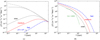 |
Fig. 3 (a) Top-of-atmosphere Galactic cosmic ray spectrum at 1 au at 200 Myr. Spectra for a slow (dotted black line), medium (dashed red line), and fast (dot-dashed blue line) solar rotation rate. The LIS is shown by the solid grey line. The enhanced LIS shown by the dot-dashed grey line is discussed in Section 4. The spectrum for the fast rotation rate has been multiplied by 102 to allow all of the spectra to be shown within a reasonable range on the same axes. (b) Top-of-atmosphere solar cosmic ray spectrum at 1 au at 200 Myr for a slow, medium, and fast solar rotation rate. The linestyles represent the same scenarios as in the Galactic cosmic ray spectra. The green line represents the fit of the observed spectrum Reeves et al. (1992) of the solar energetic particle event measured at Earth in October 1989. |
2.5 Cosmic ray transport in the atmosphere
To model the transport of cosmic rays through the early Earth atmosphere, we used the Monte Carlo model presented in Rimmer et al. (2012). With the top-of-atmosphere input cosmic ray spectra (Fig. 3) and atmospheric density profile (Fig. 2), the cosmic ray transport model distributes a number of cosmic rays, N, according to the input cosmic ray spectrum before calculating the energy losses of each cosmic ray over each increment in height above the surface, dz, down through the atmosphere. This model is based on the continuous slowing down approximation (Padovani et al. 2009) which describes the loss of energy by cosmic rays passing through a column density, n(z)dz, of a medium – in this case, the atmosphere of the early Earth. The energy lost by each cosmic ray over dz depends on the cosmic ray ‘optical depth’, τ = σ(T)ndz, over dz, where σ(T) is the ionisation cross section. For this hydrogen-dominated atmosphere, the H2 ionisation cross section described in Eqs. (5) and (6) of Padovani et al. (2009), from the fitting of experimental data presented in Rudd et al. (1985), is the dominant σ. The ionisation cross section of H2 is the only cross section we considered in our simulation setup. For the cosmic ray proton energy range considered here, 6.9 × 10⁻³ ≤ T ≤ 262 GeV, σ is larger for lower-energy cosmic rays (see Padovani et al. 2009, Fig. 1).
We use W to refer to the average cosmic ray energy loss in an ionising collision with H2 taken from Eq. (3) of Rimmer et al. (2012):
![$\[W=7.92 T^{0.82}+4.76,\]$](/articles/aa/full_html/2025/05/aa52842-24/aa52842-24-eq18.png) (7)
(7)
with T in eV. The energy loss of each cosmic ray proton is calculated by assigning a random number, A, between 0 and 1 to each cosmic ray and comparing τ with both the energy of the proton and A as follows:
If A < τ < 1, the cosmic ray loses energy W.
If
![$\[1 \leq \tau<\frac{T}{W}\]$](/articles/aa/full_html/2025/05/aa52842-24/aa52842-24-eq19.png) , the cosmic ray loses a random amount of kinetic energy between 0 and τW.
, the cosmic ray loses a random amount of kinetic energy between 0 and τW.If
![$\[\tau \geq \frac{T}{W}\]$](/articles/aa/full_html/2025/05/aa52842-24/aa52842-24-eq20.png) , the cosmic ray loses all of its kinetic energy and does not contribute to the cosmic ray flux at the next dz.
, the cosmic ray loses all of its kinetic energy and does not contribute to the cosmic ray flux at the next dz.
In our modelling of cosmic rays in the early Earth atmosphere, we used N = 500 000 and 10−3 km ≤ z ≤ 2700 km, with a logarithmically spaced z grid. The result of these calculations is a set of values of j at each energy value for each of the 250 heights in the atmosphere.
We used j(T, z) to calculate the important quantities for chemical modelling of the early Earth atmosphere – the ionisation rate of H2 and the ion-pair production rate, Q(z), discussed in Section 3.2. We calculate the ionisation rate of H2, ζ, using:
![$\[\zeta(z)=4 \pi \int_{I\left(\mathrm{H}_2\right)}^{T_{\max }} j(T, z)[1+\phi(T)] \sigma(T) d T,\]$](/articles/aa/full_html/2025/05/aa52842-24/aa52842-24-eq21.png) (8)
(8)
where I(H2) is the ionisation potential of H2 and ϕ(T) is an energy-dependent correction factor to account for ionisation by secondary electrons (e.g. Rodgers-Lee et al. 2023). Our results for j(T, z) and ζ(z) as a function of height in the early Earth atmosphere are presented in Section 3.
3 Results
In Sections 3.1 and 3.2, we present results for cosmic ray transport and the ionisation rate and ion-pair production rate of H2 by cosmic rays in the early Earth atmosphere, respectively.
3.1 Cosmic ray differential intensity
Fig. 4 shows j(T, z) for Galactic and solar cosmic rays for a range of heights in the early Earth atmosphere, for Ω = 6Ω⊙ (medium rotator case). Here we define the surface where P = 100 bar, corresponding to z = 10−3 km. The maximum height in our model is z = 2700 km (P = 10−7 bar), which we refer to as the top of the atmosphere. The cosmic ray spectra would be the same at any higher heights in the atmosphere not considered here. The values of j(T, z) at different heights are shown in grey for Galactic cosmic rays, and in red for solar cosmic rays. In the upper part of the atmosphere (z ≳ 1000 km, corresponding to P ≲ 10−1 bar) where n is low, only the lowest-energy solar cosmic rays show a decrease in j(T, z).
The energy lost by cosmic rays with kinetic energy, T, over a given dz in the atmosphere depends on σ and n. Because σ varies with T, j(T, z) changes differently with height in the atmosphere for lower and higher energy cosmic rays such that lower-energy cosmic rays (~MeV) lose larger amounts of energy due to ionising collisions than higher-energy cosmic rays (~GeV). This results in large decreases in j(T, z) with decreasing height above the surface at low values of T, given a high enough n. For solar cosmic rays at z ≤ 1000 km, there are clear decreases in j(T, z) with decreasing height, particularly at low energies (T < 1 GeV). For T > 10 GeV, j(T, z) remains approximately constant until a height of 500 km. The decreases in j(T, z) with increasing column depth for solar cosmic rays are greater when Ω is slower, due to the lower top-of-atmosphere values of j(T, z) at high energies. For example, in Fig. 3b at T = 10 GeV, there is a difference of over 105 m−2 s−1 sr−1 MeV−1 between j(T, z) for Ω = 3.5Ω⊙ and Ω = 15Ω⊙. For solar cosmic rays, there are two artificial sharp drop-offs in Fig. 4 – one above 26 GeV at z = 500 km (dashed red line), and another above 19 GeV at the surface (dot-dashed red line). At these heights, the cosmic ray flux is so low that the number of cosmic rays in the higher energy bins goes to zero due to small sample statistics.
The values of j(T, z) for Galactic cosmic rays (grey lines in Fig. 4), which have maximum top-of-atmosphere values at T > 10 GeV, remain approximately constant for z ≥ 500 km. From 500 km (dashed grey line in Fig. 4) to the surface (dot-dashed grey line) there is a small decrease in the values of j(T, z) for Galactic cosmic rays. The small change between the top-of-atmosphere and surface j(T, z) of Galactic cosmic rays is due to the fact that we only include cosmic ray energy losses due to ionisation. Since the Galactic cosmic ray spectrum peaks at high energies, where σ is smaller than at lower energies, the ionisation energy losses are small and the spectrum remains approximately constant with height. A larger change in j(T, z) between the top of the atmosphere and the surface would be expected if additional energy loss mechanisms such as those due to pion production were included (see e.g. Fig. 7 Padovani et al. 2009). For Ω = 3.5Ω⊙ and Ω = 15Ω⊙, not shown here, the results for j(T, z) show similar behaviour for Galactic cosmic rays.
The relevant quantities for chemical modelling to account for cosmic ray effects on the early Earth atmosphere are ζ (Eq. (8)) and the ion-pair production rate, Q(z) = n(z) ζ(z). In Section 3.2 we present ζ(z) and Q(z) using j(T, z).
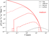 |
Fig. 4 Differential intensity, j(T, z), of solar cosmic rays (red lines) and Galactic cosmic rays (grey lines) in the early Earth atmosphere for Ω = 6Ω⊙, plotted at different heights above and at the surface as a function of T. The linestyles represent these heights (solid: top of atmosphere (TOA); dotted: 1000 km; dashed: 500 km; dot-dashed: surface). Here the surface is defined as z = 0.001 km. |
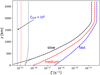 |
Fig. 5 Ionisation rate, ζ, as a function of height in the early Earth atmosphere at 200 Myr due to Galactic and solar cosmic rays. Dotted lines show ζ due to Galactic cosmic rays only, dashed lines show ζ due to solar cosmic rays only, solid lines show the total ζ from Galactic cosmic rays and solar cosmic rays combined. The ζ values for the slow, medium, and fast solar rotation rates are shown by black, red, and blue lines, respectively. For the fast solar rotation rate, ζGCR has been multiplied by 102 to allow ζGCR and ζSCR for all rotation rates to be shown within a reasonable range on the same axes. |
3.2 H2 ionisation and ion-pair production rates
Fig. 5 shows ζ (using Eq. (8)) for Galactic (ζGCR, dotted lines) and solar cosmic rays (ζSCR, dashed lines) as a function of height in the post-impact early Earth atmosphere at 200 Myr, for the three values of Ω given in Table 1. The total ζ = ζGCR + ζSCR is represented by thin solid lines. For each type of cosmic ray, the values of ζ for the slow, medium, and fast rotator cases are shown by the black, red, and blue lines, respectively.
We focus on ζ at the surface, ζsurf, to understand the effects of cosmic rays where life emerged. For the fast rotator case, taking 10−18 s−1 as an estimate for an ionisation rate high enough to have an effect on the chemistry, ζsurf ~ 10−16 s−1 resulting from solar cosmic rays is likely high enough. In the slow or medium rotator cases, ζsurf (given in Table 2) is not high enough to be important for chemistry at the surface. Thus, we find that for solar cosmic rays to be important for chemistry at the surface of the post-impact early Earth, the Sun must have been a fast rotator. We consider the suppression of the top-of-atmosphere cosmic ray spectra by a planetary magnetic field in Appendix B. We find that the suppression does not result in changes to ζsurf at 200 Myr.
On the other hand, it is possible that prebiotic molecules produced in the early Earth atmosphere could have been dissolved in atmospheric water droplets and precipitated to the surface (Benner et al. 2020). In this case, it is useful to consider ζ throughout the early Earth atmosphere. The total values of ζ at the top of the early Earth atmosphere, ζTOA, are given in Table 2. At the top of the atmosphere, ζSCR > ζGCR for all values of Ω such that ζ ≃ ζSCR. For example, for Ω = 6Ω⊙, ζSCR = 8 × 10⁻¹¹ s−1 at the top of the atmosphere, over 10 orders of magnitude higher than ζGCR = 10−21 s−1.
The top-of-atmosphere values of both ζSCR and ζGCR vary greatly depending on the value of Ω used. In the fast rotator case, ζSCR = 2 × 10⁻¹⁰ s−1 at the top of the atmosphere, nearly an order of magnitude greater than ζSCR = 3 × 10⁻¹¹ s−1 for the slow rotator. This reflects the top-of-atmosphere solar cosmic ray spectra which show higher j(T, z) for the fast rotator than for the slow rotator. The changes in ζ as a function of height are similar to the changes in j(T, z) described in Section 3.1: ζGCR is almost constant with height and ζSCR (dashed lines in Fig. 5) is large and constant in the upper atmosphere, but decreases rapidly below z = 1700 km. The decrease in ζSCR for z < 1700 km is not as rapid in the fast rotator case (dashed blue line in Fig. 5) as it is in the medium (dashed red line) and slow rotator (dashed black line) cases. This is because pmax is greater and the decrease in j(T, z) with decreasing z at low energies is more gradual for faster Ω. For the fast rotator, ![$\[\zeta_{\mathrm{SCR}}^{\text {surf}}\]$](/articles/aa/full_html/2025/05/aa52842-24/aa52842-24-eq22.png) = 1 × 10⁻¹⁶ s−1. For the slow rotator,
= 1 × 10⁻¹⁶ s−1. For the slow rotator, ![$\[\zeta_{\mathrm{SCR}}^{\text {surf}}\]$](/articles/aa/full_html/2025/05/aa52842-24/aa52842-24-eq23.png) = 2 × 10⁻²³ s−1 is lower than ζGCR = 5 × 10⁻²¹ s−1 · ζ is indistinguishable from ζSCR in Fig. 5, except for z ≲ 300 km for the slow rotator, where ζSCR < ζGCR. This suggests that solar cosmic rays have a greater effect on chemistry throughout the early Earth atmosphere than Galactic cosmic rays.
= 2 × 10⁻²³ s−1 is lower than ζGCR = 5 × 10⁻²¹ s−1 · ζ is indistinguishable from ζSCR in Fig. 5, except for z ≲ 300 km for the slow rotator, where ζSCR < ζGCR. This suggests that solar cosmic rays have a greater effect on chemistry throughout the early Earth atmosphere than Galactic cosmic rays.
Fig. 6 shows Q(z) in the early Earth atmosphere for both Galactic (QGCR, dotted red line) and solar (QSCR, dashed red line) cosmic rays for Ω = 6Ω⊙ (medium rotator case). The total Q = QGCR + QSCR as a function of height is shown by the solid black line. For comparison, for the present-day Earth, balloon measurements by Neher (1971) for 16th April 1965 covering 6 km < z < 32 km showed a maximum of Q = 37.48 cm−3 s−1 at z = 14 km. Similar to ζ, QSCR ≫ QGCR for Ω = 6Ω⊙ at all heights and the total Q is indistinguishable from QSCR. The maximum value of QSCR is at z = 150 km (P = 50 bar). If additional energy losses such as those due to pion production were included, ζGCR would decrease with decreasing height and lead to the maximum of QGCR occurring at some z in the atmosphere and not in the soil as our results currently suggest. Air shower models such as AtRIS (Banjac et al. 2019) can be used in the future to include these additional energy losses.
The values of QSCR and QGCR presented in Fig. 6 indicate that solar cosmic rays are more important for chemistry than Galactic cosmic rays at all heights in the early Earth atmosphere for Ω = 6Ω⊙. Similarly, QSCR > QGCR throughout the atmosphere for Ω = 15Ω⊙. For Ω = 3.5Ω⊙, QGCR > QSCR for z ≤ 300 km (P ≥ 20 bar), where ζ < 1019s−1 appears too low to have a significant effect on the atmospheric chemistry.
4 Discussion
4.1 Variations of the Galactic cosmic ray spectrum
The Galactic cosmic ray results in Sections 3.1–3.2 are based on the assumption that the LIS is approximately constant on gigayear timescales (ignoring short-term effects related to the solar cycle, Potgieter 2013). However, there are a number of factors that can change the Galactic cosmic ray spectrum both spatially and temporally in the Galaxy. Firstly, the Galactic cosmic ray spectrum is different inside and outside the Galaxy’s spiral arms. The model presented by Büsching & Potgieter (2008) showed approximately a factor of 2 increase in cosmic ray fluxes inside the spiral arms compared to the inter-arm regions due to cosmic ray sources, assumed to be supernova remnants, in the spiral arms. This is in agreement with γ-ray observations – Aharonian et al. (2020) find an increase by a factor of 2–4 in the flux of cosmic rays with energies >10 GeV within 100 pc of supernova remnants, compared to the homogeneous ‘sea’ of cosmic rays observed throughout the Galaxy. The rate of supernova remnants, which is dependent on the star formation rate in the Galaxy, would also have influenced the Galactic cosmic ray spectrum on gigayear timescales. Assuming that the Galactic cosmic ray flux is proportional to the star formation rate in the Galaxy, Svensmark (2006) indicated a factor of 1.4 increase in the Galactic cosmic ray flux at 200 Myr compared to the present day due to the increased supernova remnant/star formation rate.
The presence of young low-mass stars in star-forming regions will also influence the Galactic cosmic ray spectrum, mainly at ~MeV energies. Here we investigate the effect of varying the LIS to reflect this influence on the top-of-atmosphere values of j(T) and ζGCR(z) for the early Earth. Because the majority of stars form within star clusters (Arakawa & Kokubo 2023), it is likely that there were many young low-mass stars close to the Sun at 200 Myr. Taking cosmic rays accelerated at these young low-mass stars into account (e.g. Padovani et al. 2016), j(T) in the LIS was likely higher than at present, particularly at ~MeV energies (shown by the dot-dashed grey line in Fig. 3a as ![$\[j_{\text {LIS }}^{\text {high}}\]$](/articles/aa/full_html/2025/05/aa52842-24/aa52842-24-eq24.png) Padovani et al. 2018).
Padovani et al. 2018). ![$\[j_{\text {LIS }}^{\text {high}}\]$](/articles/aa/full_html/2025/05/aa52842-24/aa52842-24-eq25.png) (T) has higher values than jLIS (Eq. (5)) at low energies to reproduce the cosmic ray ionisation rates observed in molecular clouds, that cannot be explained by a simple extrapolation of Voyager 1 data to low energies and are likely due to increased cosmic ray production from nearby young lowmass stars. This spectrum, labelled ℋ in Padovani et al. (2018), is given by:
(T) has higher values than jLIS (Eq. (5)) at low energies to reproduce the cosmic ray ionisation rates observed in molecular clouds, that cannot be explained by a simple extrapolation of Voyager 1 data to low energies and are likely due to increased cosmic ray production from nearby young lowmass stars. This spectrum, labelled ℋ in Padovani et al. (2018), is given by:
![$\[j_{\mathrm{LIS}}^{\text {high }}(T)=2.4 \times 10^{15} \frac{T^{-0.8}}{\left(T+T_0\right)^{1.9}} \mathrm{eV}^{-1} \mathrm{s}^{-1} \mathrm{cm}^{-2} \mathrm{sr}^{-1},\]$](/articles/aa/full_html/2025/05/aa52842-24/aa52842-24-eq26.png) (9)
(9)
where T0 = 6.50 × 10⁸ eV and T is in units of eV.
Using the same solar wind properties (Table 2) and cosmic ray transport model as in Section 2.3, we have produced new Galactic cosmic ray spectra at different orbital distances using ![$\[j_{\text {LIS }}^{\text {high}}\]$](/articles/aa/full_html/2025/05/aa52842-24/aa52842-24-eq27.png) (T). Ignoring the effect of a planetary magnetic field, these spectra would be the hypothetical top-of-atmosphere spectra at these orbital distances. Fig. 7 shows ζGCR at the top of the early Earth atmosphere,
(T). Ignoring the effect of a planetary magnetic field, these spectra would be the hypothetical top-of-atmosphere spectra at these orbital distances. Fig. 7 shows ζGCR at the top of the early Earth atmosphere, ![$\[\zeta_{\mathrm{GCR}}^{\mathrm{TOA}}\]$](/articles/aa/full_html/2025/05/aa52842-24/aa52842-24-eq28.png) , as a function of orbital distance, r, calculated using the hypothetical top-of-atmosphere spectra. We compare
, as a function of orbital distance, r, calculated using the hypothetical top-of-atmosphere spectra. We compare ![$\[\zeta_{\mathrm{GCR}}^{\mathrm{TOA}}\]$](/articles/aa/full_html/2025/05/aa52842-24/aa52842-24-eq29.png) resulting from jLIS (circles) and
resulting from jLIS (circles) and ![$\[j_{\text {LIS }}^{\text {high}}\]$](/articles/aa/full_html/2025/05/aa52842-24/aa52842-24-eq30.png) (crosses), for the medium rotator case as an example.
(crosses), for the medium rotator case as an example.
We find at 1 au, where the low-energy part of the Galactic cosmic ray spectrum is suppressed due to the solar wind, that the spectrum is unchanged by varying the LIS. Thus, ![$\[\zeta_{\mathrm{GCR}}^{\mathrm{TOA}}\]$](/articles/aa/full_html/2025/05/aa52842-24/aa52842-24-eq34.png) for the medium rotation rate is the same (
for the medium rotation rate is the same (![$\[\zeta_{\mathrm{GCR}}^{\mathrm{TOA}}\]$](/articles/aa/full_html/2025/05/aa52842-24/aa52842-24-eq35.png) = 10−21 s−1) for both
= 10−21 s−1) for both ![$\[j_{\text {LIS }}^{\text {high}}\]$](/articles/aa/full_html/2025/05/aa52842-24/aa52842-24-eq36.png) and jLIS, indicating that an increase in jLIS at low energies would not have a significant effect on ζGCR in Earth’s atmosphere at 200 Myr for the scenario considered here. The low-energy Galactic cosmic rays at 1 au are not in fact related to the low-energy LIS cosmic rays. Instead, j at low energies at 1 au depends on j in the LIS at higher energies. The high-energy Galactic cosmic rays propagating through the Solar System experience energy losses when doing work against the solar wind and contribute to j at lower energies at 1 au.
and jLIS, indicating that an increase in jLIS at low energies would not have a significant effect on ζGCR in Earth’s atmosphere at 200 Myr for the scenario considered here. The low-energy Galactic cosmic rays at 1 au are not in fact related to the low-energy LIS cosmic rays. Instead, j at low energies at 1 au depends on j in the LIS at higher energies. The high-energy Galactic cosmic rays propagating through the Solar System experience energy losses when doing work against the solar wind and contribute to j at lower energies at 1 au.
More generally, for r < 1300au, the top-of-atmosphere spectra resulting from jLIS and ![$\[j_{\text {LIS }}^{\text {high}}\]$](/articles/aa/full_html/2025/05/aa52842-24/aa52842-24-eq37.png) are similar – the difference between
are similar – the difference between ![$\[\zeta_{\mathrm{GCR}}^{\mathrm{TOA}}\]$](/articles/aa/full_html/2025/05/aa52842-24/aa52842-24-eq38.png) calculated using the two top-of-atmosphere spectra does not exceed 10%. However, Fig. 7 shows that
calculated using the two top-of-atmosphere spectra does not exceed 10%. However, Fig. 7 shows that ![$\[\zeta_{\mathrm{GCR}}^{\mathrm{TOA}}\]$](/articles/aa/full_html/2025/05/aa52842-24/aa52842-24-eq39.png) derived from jLIS(T) is slightly greater than
derived from jLIS(T) is slightly greater than ![$\[\zeta_{\mathrm{GCR}}^{\mathrm{TOA}}\]$](/articles/aa/full_html/2025/05/aa52842-24/aa52842-24-eq40.png) derived from
derived from ![$\[j_{\text {LIS }}^{\text {high }}\]$](/articles/aa/full_html/2025/05/aa52842-24/aa52842-24-eq41.png) (T) for r < 1300 au. The small differences are due to the slightly lower values of
(T) for r < 1300 au. The small differences are due to the slightly lower values of ![$\[j_{\text {LIS }}^{\text {high }}\]$](/articles/aa/full_html/2025/05/aa52842-24/aa52842-24-eq42.png) (T) compared to jLIS(T) at high energies, visible for T > 5 GeV in Fig. 3a.
(T) compared to jLIS(T) at high energies, visible for T > 5 GeV in Fig. 3a.
However, for hypothetical planets orbiting at r ⩾ 1300 au, the effect on ![$\[\zeta_{\mathrm{GCR}}^{\mathrm{TOA}}\]$](/articles/aa/full_html/2025/05/aa52842-24/aa52842-24-eq43.png) of varying the LIS of Galactic cosmic rays is greater. Compared to jLIS,
of varying the LIS of Galactic cosmic rays is greater. Compared to jLIS, ![$\[j_{\text {LIS }}^{\text {high }}\]$](/articles/aa/full_html/2025/05/aa52842-24/aa52842-24-eq44.png) (T) is larger for low-energy Galactic cosmic rays. At large values of r, the suppression of Galactic cosmic rays is not extreme enough to make this difference insignificant in the modelled top-of-atmosphere spectra. The higher intensity of low-energy cosmic rays with large ionisation cross-sections results in a higher
(T) is larger for low-energy Galactic cosmic rays. At large values of r, the suppression of Galactic cosmic rays is not extreme enough to make this difference insignificant in the modelled top-of-atmosphere spectra. The higher intensity of low-energy cosmic rays with large ionisation cross-sections results in a higher ![$\[\zeta_{\mathrm{GCR}}^{\mathrm{TOA}}\]$](/articles/aa/full_html/2025/05/aa52842-24/aa52842-24-eq45.png) · At 2300 au,
· At 2300 au, ![$\[\zeta_{\mathrm{GCR}}^{\mathrm{TOA}}\]$](/articles/aa/full_html/2025/05/aa52842-24/aa52842-24-eq46.png) calculated using the top-of-atmosphere spectrum resulting from
calculated using the top-of-atmosphere spectrum resulting from ![$\[j_{\text {LIS }}^{\text {high}}\]$](/articles/aa/full_html/2025/05/aa52842-24/aa52842-24-eq47.png) (T) is a factor of 3 larger than the value calculated using the spectrum resulting from jLIS. Outside of the Solar System,
(T) is a factor of 3 larger than the value calculated using the spectrum resulting from jLIS. Outside of the Solar System, ![$\[j_{\text {LIS }}^{\text {high }}\]$](/articles/aa/full_html/2025/05/aa52842-24/aa52842-24-eq48.png) = 10−16 s−1, which is an order of magnitude greater than ζLIS = 10−17 s−1. For the slow rotator case, the effect of changing the LIS is seen at smaller orbital distances. For r < 400 au,
= 10−16 s−1, which is an order of magnitude greater than ζLIS = 10−17 s−1. For the slow rotator case, the effect of changing the LIS is seen at smaller orbital distances. For r < 400 au, ![$\[\zeta_{\mathrm{GCR}}^{\mathrm{TOA}}\]$](/articles/aa/full_html/2025/05/aa52842-24/aa52842-24-eq49.png) calculated using both top-of-atmosphere spectra are similar. The factor of 3 increase in
calculated using both top-of-atmosphere spectra are similar. The factor of 3 increase in ![$\[\zeta_{\mathrm{GCR}}^{\mathrm{TOA}}\]$](/articles/aa/full_html/2025/05/aa52842-24/aa52842-24-eq50.png) when using
when using ![$\[j_{\text {LIS }}^{\text {high}}\]$](/articles/aa/full_html/2025/05/aa52842-24/aa52842-24-eq51.png) (T) seen at 2300 au for the medium rotator case occurs at ~1400 au for the slow rotator case.
(T) seen at 2300 au for the medium rotator case occurs at ~1400 au for the slow rotator case.
We find that assuming a LIS which changes at lower energies over gigayear timescales has a minimal impact on the calculated ionisation rate at 1 au. To affect ![$\[\zeta_{\mathrm{GCR}}^{\mathrm{TOA}}\]$](/articles/aa/full_html/2025/05/aa52842-24/aa52842-24-eq52.png) at 1 au, the LIS would need to have higher j values compared to jLIS at higher energies (T > 1 GeV). This could be caused by the acceleration of Galactic cosmic rays by a nearby supernova remnant. At larger orbital distances, where Galactic cosmic rays are subject to less extreme suppression, the LIS used has a greater effect on the resulting ionisation rate at the top of the atmosphere. When comparing ζGCR and ζSCR for exoplanets orbiting at large distances from their host stars, it will be important to consider the Galactic cosmic ray spectra resulting from different possible LIS. The stellar wind properties of the host star will also play an important role in determining the suppression of the Galactic cosmic ray spectrum and the orbital distance at which a change in the LIS affects
at 1 au, the LIS would need to have higher j values compared to jLIS at higher energies (T > 1 GeV). This could be caused by the acceleration of Galactic cosmic rays by a nearby supernova remnant. At larger orbital distances, where Galactic cosmic rays are subject to less extreme suppression, the LIS used has a greater effect on the resulting ionisation rate at the top of the atmosphere. When comparing ζGCR and ζSCR for exoplanets orbiting at large distances from their host stars, it will be important to consider the Galactic cosmic ray spectra resulting from different possible LIS. The stellar wind properties of the host star will also play an important role in determining the suppression of the Galactic cosmic ray spectrum and the orbital distance at which a change in the LIS affects ![$\[\zeta_{\mathrm{GCR}}^{\mathrm{TOA}}\]$](/articles/aa/full_html/2025/05/aa52842-24/aa52842-24-eq53.png) . For example, keeping the level of turbulence constant, an increased stellar wind velocity increases the suppression of the Galactic cosmic ray spectrum and a change in the LIS produces a change in
. For example, keeping the level of turbulence constant, an increased stellar wind velocity increases the suppression of the Galactic cosmic ray spectrum and a change in the LIS produces a change in ![$\[\zeta_{\mathrm{GCR}}^{\mathrm{TOA}}\]$](/articles/aa/full_html/2025/05/aa52842-24/aa52842-24-eq54.png) at a greater orbital distance. Investigating ionisation due to cosmic rays in exoplanet atmospheres orbiting at large distances from a host star with a stellar wind similar to the young Sun requires knowledge of the LIS.
at a greater orbital distance. Investigating ionisation due to cosmic rays in exoplanet atmospheres orbiting at large distances from a host star with a stellar wind similar to the young Sun requires knowledge of the LIS.
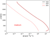 |
Fig. 6 Ion-pair production rate, Q, as a function of height in the early Earth atmosphere at 200 Myr for Ω = 6Ω⊙. The solid black line shows the total Q value: the sum of Q for Galactic cosmic rays (‘GCR’, dotted red line) and for solar cosmic rays (‘SCR’, dashed red line). |
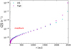 |
Fig. 7
|
![$\[\zeta_{\mathrm{GCR}}^{\mathrm{TOA}}\]$](/articles/aa/full_html/2025/05/aa52842-24/aa52842-24-eq31.png)
![$\[\zeta_{\mathrm{GCR}}^{\mathrm{TOA}}\]$](/articles/aa/full_html/2025/05/aa52842-24/aa52842-24-eq32.png)
![$\[j_{\text {LIS }}^{\text {high }}\]$](/articles/aa/full_html/2025/05/aa52842-24/aa52842-24-eq33.png)
4.2 Importance for chemistry and exoplanet atmospheres
The influence of cosmic rays on the chemistry of (exo)planetary atmospheres is relevant both for the search for signatures of life on exoplanets and the study of the origin of life on Earth. Rodgers-Lee et al. (2023) model the transport of stellar and Galactic cosmic rays through the H2-dominated atmosphere of a gas giant with an M dwarf host star. The result shown in Fig. 6 of Rodgers-Lee et al. (2023) is that stellar cosmic rays dominate until the atmospheric pressure exceeds 10 bar, and QGCR (P = 100 bar) ≃ 1 cm−3 s−1. This result is similar to the slow rotator case for the early Earth atmosphere discussed here, where QSCR > QGCR for P < 20 bar and QGCR (P = 100 bar = 10 cm−3 s−1. Modelling of M dwarf exoplanet systems (e.g. Herbst et al. 2020; Mesquita et al. 2021, 2022) has focused on the 1D transport and role of cosmic rays in these systems. Studying exoplanets observable with JWST transmission spectroscopy can provide more information on the cosmic ray effects on atmospheres similar to the early Earth atmosphere and improve our understanding of the origin of life.
Rimmer & Helling (2016) present an ion-neutral chemical model, used to study the chemical reactions in a selection of atmospheres including an early Earth atmosphere dominated by CO2 and N2. Along with chemistry driven by UV light and lightning, this model takes into account chemistry driven by cosmic ray ionisation. The cosmic ray ionisation rate in the atmosphere is therefore an important input. Chemical modelling (e.g. Helling & Rimmer 2019) shows that cosmic ray ionisation is important for producing molecules such as H3O+ and enhancing prebiotic molecule production (Barth et al. 2021). Our results can be used in chemical models to improve our understanding of prebiotic chemistry in the post-impact early Earth scenario investigated here. In the future, to use our results for ζ in chemical modelling, it would be important for the chemical models to include all of the relevant molecular abundances in the atmosphere, such as those given in Table 1 of Zahnle et al. (2020) for CO2, CH4 and NH3 in addition to the H2 included here in the cosmic ray model.
The effects of cosmic rays on the chemistry of H2-dominated atmospheres are relevant in the search for the chemical signatures of life on exoplanets (see e.g. Herbst et al. 2022, for a recent review). The upper atmosphere becomes relevant when considering the applications of cosmic ray transport modelling beyond Earth. Exoplanets observable by JWST (Dyrek et al. 2024; Gardner et al. 2006; Rigby et al. 2023) include warm Neptune planets with H2-dominated atmospheres (e.g. Rodgers-Lee et al. 2023). The effects of cosmic rays on the chemistry of the upper atmospheres of these exoplanets are important for interpreting transmission spectroscopy observations probing low pressures (Welbanks & Madhusudhan 2019). Hycean worlds – planets with potentially habitable ocean surfaces underneath H2-rich atmospheres – are promising candidates for the detection of biosignatures using JWST NIRSpec and NIRISS transmission spectroscopy (Madhusudhan et al. 2021). There has been much interest in JWST observations of the exoplanet K2-18 b, which has been interpreted as a Hycean world (Madhusudhan et al. 2023) and later as a gas giant with no habitable surface (Wogan et al. 2024). The interpretation of observations of exoplanets orbiting active stars using chemical models may be affected by the high stellar cosmic ray ionisation expected in the exoplanet atmospheres.
Additionally, the H2-dominated atmospheres of exoplanets in diverse environments act as ‘laboratories’ to search for prebiotic chemistry (Rimmer & Helling 2016) where observations of the early Earth atmosphere itself are not possible. Claringbold et al. (2023) find that prebiotic molecules such as cyanoacetylene and formaldehyde are well suited for detection in H2-rich exoplanet atmospheres, such as Hycean worlds and post-impact planets, using the JWST NIRSpec and NIRISS instruments. The results presented by Claringbold et al. (2023) emphasise the strong capabilities of JWST transmission spectroscopy observations of H2-dominated exoplanet atmospheres to advance the study of the origin of life.
4.3 Additional cosmic ray effects
The transport model described in this paper takes into account the energy lost by cosmic rays through ionising collisions. For the energy range (10−2 GeV ≲ T ≲ 102 GeV) discussed in this paper, the ionisation cross section is larger for lower-energy cosmic rays and the higher-energy cosmic rays reach deeper into the atmosphere before losing energy to ionisation collisions. The model adopted here does not take into account the additional energy lost to pion production by cosmic ray protons with energies above ~1 GeV (see Fig. 7 of Padovani et al. 2009). Pion production is only a first step in a cascade or air shower, where secondary particles are produced and go on to have additional effects on the chemistry in the atmosphere. The particle transport model presented by Herbst et al. (2019) includes secondary particle effects on chemistry in the present-day Earth’s atmosphere. Above ~1 GeV the energy lost to pion production increases with increasing cosmic ray proton energy (e.g. Padovani et al. 2009), suggesting that the differential intensity in the post-impact early Earth atmosphere presented here may be an overestimation for higher-energy cosmic rays reaching the surface. However, experiments studying different early Earth atmosphere compositions including CO, CO2, N2, and H2O show that the secondary electrons produced by these high-energy cosmic rays are also interesting because they can break N2 bonds and lead to increased production of HCN (Airapetian et al. 2020).
Other secondary cosmic ray particles such as muons interact with prebiotic molecules and can produce additional changes to these molecules. Globus & Blandford (2020) suggest that interactions between spin-polarised cosmic ray muons and biological molecules is one explanation for the chirality of DNA and RNA helices. Future calculations of the secondary particle fluxes associated with our cosmic ray proton spectra in the early Earth atmosphere would provide further insight into the role of cosmic rays in the origin of life.
5 Conclusions
In this paper, we model the transport of Galactic and solar cosmic rays in a transient H2-dominated atmosphere after an oceanvaporising impact, known as the post-impact early Earth atmosphere. This atmosphere, low in oxygen, presents a favourable environment for the formation of prebiotic molecules, if a source of ionisation is also present. Our aim is to compare ionisation by Galactic and solar cosmic rays in the early Earth atmosphere, particularly at the surface where life likely formed. To achieve this, we calculated the differential intensity of Galactic and solar cosmic rays separately as a function of height in the atmosphere. We calculated the resulting H2 ionisation rates as a function of atmospheric height. The Galactic and solar cosmic ray spectra arriving at the Earth are determined by the properties of the Sun and solar wind, which both depend on the Sun’s rotation rate. For the post-impact early Earth scenario at 200 Myr, the Sun’s rotation rate is unknown. To represent the range of possible rotation rates of the young Sun, we modelled the cosmic ray spectra in three scenarios – slow (Ω = 3.5Ω⊙), medium (Ω = 6Ω⊙), and fast (Ω = 15Ω⊙) rotator cases, spanning the range of observed rotation rates for low-mass stars.
For each of the three assumed solar rotation rates, the differential intensity of Galactic cosmic rays at the top of the early Earth atmosphere is at its maximum at high energies (T > 1 GeV). These high-energy cosmic rays lose little energy to ionisation in the atmosphere, resulting in Galactic cosmic ray spectra at the surface which are similar to the top-of-atmosphere spectra. In contrast, solar cosmic rays have maximum top-of-atmosphere differential intensities at low energies (T < 1 GeV). At low energies, the differential intensity decreases with decreasing height, producing solar cosmic ray spectra which differ in both overall differential intensity and shape compared to the top-of-atmosphere spectra.
We find that for each of the three solar rotation rates, the ionisation rate throughout the atmosphere, except for z ≲ 300 km for the slow rotator case, is dominated by solar cosmic rays. However, only in the fast rotator case is the ionisation rate at the surface (ζsurf~10−16 s−1) high enough to be of interest for chemistry. The ion-pair production rate reaches its maximum in the lower part of atmosphere, ~100–300 km above the surface. For all three solar rotation rates, the ion-pair production rate at its maximum is also dominated by solar cosmic rays. Galactic cosmic rays become dominant – but not of interest for chemistry – only for the slow rotator case, for z < 300 km.
We consider the effect of the Earth’s magnetic field on the top-of-atmosphere cosmic ray spectra. Low-energy cosmic rays are affected by Earth’s magnetic field and are deflected towards the poles. This deflection particularly affects lower-energy cosmic rays below a cutoff energy. We calculated the cutoff energy imposed on the top-of-atmosphere cosmic ray spectra by the early Earth’s magnetic field to be TC = 2.56 GeV. We modified the top-of atmosphere spectra to account for the deflection of cosmic rays with energies below this cutoff. High-energy (T > 2.5 GeV) cosmic rays are not deflected. At the surface, the ionisation rate is not related to the low-energy part of the top-of-atmosphere spectrum, and is not affected by the suppression of this spectrum at low energies.
These results assume that the spectrum of Galactic cosmic rays outside the Solar System is constant over gigayear timescales. To account for the possibility of young low-mass stars near the Solar System at 200 Myr increasing the flux of low-energy (T < 1 GeV) cosmic rays compared to today, we compared the top-of-atmosphere ionisation rate by Galactic cosmic rays using the present-day local interstellar spectrum and a spectrum which has increased cosmic ray flux at low energies (more than a factor of 10 larger at 10−2 GeV). Interestingly, at 1 au this change to the low-energy end of the LIS has no effect on the Galactic cosmic ray ionisation rate. At larger orbital distances, where the suppression of the LIS by the solar wind is less severe, the difference becomes more significant – for Ω = 6Ω⊙ at 2300 au the ionisation rate is a factor of 3 larger when using the higher LIS. For applications of cosmic ray transport modelling to exoplanet systems with a stellar wind similar to the young Sun and a fixed level of turbulence, the use of a different LIS is likely to affect the resulting top-of-atmosphere cosmic ray spectra only at large orbital distances.
The fact that the top-of-atmosphere Galactic cosmic ray spectra at 1 au resulted in extremely low ionisation rates depends on the turbulence and ISM properties adopted. 3D particle drift effects that are not captured in our 1D transport model could lead to an increase in the top-of-atmosphere Galactic cosmic ray fluxes and warrants further 3D transport modelling in the future. At the same time, we find that in the post-impact early Earth atmosphere, solar cosmic rays are an important source of ionisation that should be taken into account for planetary chemical modelling in the future. Solar cosmic rays dominate the ionisation rate throughout the planet’s atmosphere. Depending on the rotation rate of the young Sun, we find that this ionisation can be high enough to significantly alter the chemistry down on the Earth’s surface.
Acknowledgements
We thank the anonymous reviewer for their constructive comments which improved the paper. SRR and DRL would like to acknowledge that this publication has emanated from research conducted with the financial support of Taighde Éireann – Research Ireland under Grant number 21/PATHS/9339. SRR would like to thank Andrew Taylor and Tom Ray for helpful discussions which improved the paper.
Appendix A Pressure-altitude plot
Fig. A.1 shows pressure as a function of altitude for the postimpact early Earth atmosphere (solid line) and for the present-day Earth atmosphere (dashed line). The steeper decrease in P with increasing z for the present-day Earth atmosphere compared to the early Earth atmosphere is related to the scale height in each case as described in Section 2.1.
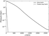 |
Fig. A.1 Pressure-altitude plot for a post-impact early Earth atmosphere (solid line) and for the present-day Earth (dashed line). |
Appendix B Impact of planetary magnetic field on cosmic ray spectra
Because cosmic rays are charged particles, they are deflected while moving in magnetic fields. There have been numerous studies on the trajectory of cosmic rays in planetary magnetic fields, since Størmer’s work on trajectories of charged particles which are either reflected or penetrate Earth’s atmosphere (Størmer 1955). Computing the trajectories of particles with a given rigidity, R = p/q (where p is the particle’s momentum and q its charge), through a model of the Earth’s magnetic field is used to explain the number of reflected or penetrating cosmic rays (Shea et al. 1987). Above a cutoff rigidity, RC, at a given location, there are no more reflected trajectories. Below RC, j(T) becomes more suppressed with decreasing R as the number of reflected trajectories increases. To approximate RC at a given geomagnetic latitude, λ, we use the Størmer cutoff rigidity (Størmer 1955), given by:
![$\[R_{\mathrm{C}}=\frac{M \cos ^4 \lambda}{4 r_{\oplus}^2},\]$](/articles/aa/full_html/2025/05/aa52842-24/aa52842-24-eq55.png) (B.1)
(B.1)
where M (G · cm3) is the Earth’s magnetic dipole moment, r⊕ (cm) is the Earth’s radius, and RC is in statvolts. This approximation is only valid for λ > 60° (Pilchowski et al. 2010). We calculate RC at λ = 60° as the extreme limit for this approximation to illustrate the greatest level of suppression. At higher latitudes, as λ → 90°, RC → 0 and the unsuppressed spectrum is recovered.
More complex models using trajectory tracing (e.g. Smart et al. 2000; Herbst et al. 2013) have been used to investigate the effect of the planetary magnetic field on cosmic ray propagation in the present-day Earth atmosphere, including at low latitudes. These studies use models of Earth’s magnetic field to calculate RC throughout the atmosphere. As a first step, for Earth at 200 Myr, we used Eq. (B.1) to give an indication of the possible effect of a planetary magnetic field on the cosmic ray spectra in the early Earth atmosphere. We used a value of the Earth’s surface magnetic field strength in the equatorial region of B⊕ = 0.13G for the early Earth1 (Tarduno et al. 2020). For comparison, at present in the equatorial region B⊕ ~ 0.3G (Finlay et al. 2010; Varela et al. 2023). From Eq. (B.1) and M = B⊕r⊕3, we obtained RC = 0.74 GV for λ = 60°. For protons this corresponds to a cutoff energy, TC = 0.74GeV.
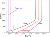 |
Fig. B.1 Ionisation rate, ζ, as a function of height in the early Earth atmosphere at 200 Myr due to Galactic and solar cosmic rays, with TC = 0.74GeV. The linestyles are the same as in Fig. 5. We use the same axes as Fig. 5 for the purpose of comparison. |
For T < TC, j(T) is suppressed but not zero. The suppression of the cosmic ray spectra for T < TC depends on both T and λ. This can be seen in the AMS-01 measurements of cosmic rays taken at different latitudes for z ~ 320–390 km, presented in Fig. 4.9 from Aguilar et al. (2002). To approximate the suppression of the cosmic ray spectra for T < TC shown in Aguilar et al. (2002), we used the suppression function:
![$\[j_{\text {supp }}(T)=\frac{j(T)}{2}\left(1-\tanh \left(a \frac{T_{\mathrm{C}}}{T}-b\right)\right),\]$](/articles/aa/full_html/2025/05/aa52842-24/aa52842-24-eq56.png) (B.2)
(B.2)
where a = 3.7–2.5Θ, b = 2, and Θ (radians) is the geomagnetic latitude. We then modelled the propagation of the cosmic rays through the post-impact early Earth atmosphere and calculated ζ(z) as previously described in Section 2.5.
Figure B.1 shows ζ(z) in the post-impact early Earth atmosphere at 200 Myr for solar and Galactic cosmic rays suppressed by a planetary magnetic field with B⊕ = 0.13G and TC = 0.74GeV. The linestyles are the same as in Fig. 5.
For solar cosmic rays in the upper atmosphere, the high ζSCR shown in Fig. 5 due to the high j(T, z) at low energies is decreased by several orders of magnitude in the presence of the planetary magnetic field. For Ω = 15Ω⊙ at the top of the atmosphere, ζSCR = 2 × 10⁻¹⁰ s−1, decreasing to ζSCR = 2 × 10⁻¹² s−1 when the spectrum is suppressed by the planetary magnetic field. Additionally, ζSCR remains constant deeper into the atmosphere (until z < 1000km). For comparison, ζSCR shown in Fig. 5 begins to decrease with decreasing z when z < 1700 km. Closer to the surface (z < 1000km), ζSCR is determined by j(T, z) of the higher-energy (T > TC) cosmic rays. At these higher energies T > TC and ζSCR is unchanged compared to the results presented in Section 3.2.
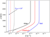 |
Fig. B.2 Ionisation rate, ζ, as a function of height in the early Earth atmosphere at 200 Myr due to Galactic and solar cosmic rays, with TC = 2.56GeV. The linestyles are the same as in Fig. 5. We use the same axes as Fig. 5 for the purpose of comparison. |
To account for the possibility of a stronger planetary magnetic field for the early Earth we used a value of the Earth’s surface magnetic field strength in the equatorial region of B⊕ = 0.45G (Varela et al. 2023). For λ = 60° for protons this corresponds to a cutoff energy, TC = 2.56GeV.
Figure B.2 shows ζ(z) in the post-impact early Earth atmosphere at 200 Myr for solar and Galactic cosmic rays suppressed by a planetary magnetic field with B⊕ = 0.45G and TC = 2.56GeV. The linestyles are the same as in Fig. 5.
For solar cosmic rays in the upper atmosphere, the high ζSCR shown in Fig. 5 due to the high j(T, z) at low energies is decreased by several orders of magnitude in the presence of the planetary magnetic field. For Ω = 15Ω⊙ at the top of the atmosphere, ζSCR = 2 × 10⁻¹⁰ s−1, decreasing to ζSCR = 1 × 10⁻¹² s−1 when the spectrum is suppressed by the planetary magnetic field. Additionally, ζSCR remains constant deeper into the atmosphere (until z < 1000km). For comparison, ζSCR shown in Fig. 5 begins to decrease with decreasing z when z < 1700 km. Closer to the surface (z < 1000km), ζSCR is determined by j(T, z) of the higher-energy (T > TC) cosmic rays. At these higher energies, T > TC and ζSCR is unchanged compared to the results presented in Section 3.2. Similar to the TC = 0.74GeV scenario, ζSCR at the top of the atmosphere is decreased by several orders of magnitude for TC = 2.56GeV. For Ω = 15Ω⊙ at the top of the atmosphere, ζSCR = 2 × 10⁻¹⁰ s−1, decreasing to ζSCR = 3 × 10⁻¹³ s−1 when TC = 2.56GeV. At the surface, ζSCR is unchanged compared to the results presented in Section 3.2.
For Galactic cosmic rays for both TC = 0.74GeV and TC = 2.56GeV, compared to the results presented in Section 3.2, ζGCR is unchanged by the planetary magnetic field. The Galactic cosmic ray spectra have maximum j(T, z) at high energies (T > TC) and low j(T, z) for T ≲ TC.
Overall, we find that the suppression of the top-of-atmosphere cosmic ray spectra at 200 Myr by B⊕ does not result in a decreased ζ near the surface compared to the results described in Section 3.2.
References
- Aguilar, M., Alcaraz, J., Allaby, J., et al. 2002, Phys. Rep., 366, 331 [NASA ADS] [CrossRef] [Google Scholar]
- Aharonian, F., Peron, G., Yang, R., Casanova, S., & Zanin, R. 2020, Phys. Rev. D, 101, 083018 [NASA ADS] [CrossRef] [Google Scholar]
- Airapetian, V. S., Glocer, A., Gronoff, G., Hébrard, E., & Danchi, W. 2016, Nat. Geosci., 9, 452 [Google Scholar]
- Airapetian, V. S., Barnes, R., Cohen, O., et al. 2020, Int. J. Astrobiol., 19, 136 [NASA ADS] [CrossRef] [Google Scholar]
- Arakawa, S., & Kokubo, E. 2023, A&A, 670, A105 [NASA ADS] [CrossRef] [EDP Sciences] [Google Scholar]
- Banjac, S., Herbst, K., & Heber, B. 2019, J. Geophys. Res. (Space Phys.), 124, 50 [Google Scholar]
- Barth, P., Helling, C., Stüeken, E. E., et al. 2021, MNRAS, 502, 6201 [Google Scholar]
- Bell, A. R. 1978, MNRAS, 182, 147 [Google Scholar]
- Bellotti, S., Fares, R., Vidotto, A. A., et al. 2023, A&A, 676, A139 [NASA ADS] [CrossRef] [EDP Sciences] [Google Scholar]
- Benner, S. A., Kim, H.-J., & Biondi, E. 2019, Life, 9, 84 [Google Scholar]
- Benner, S. A., Bell, E. A., Biondi, E., et al. 2020, ChemSystemsChem, 2, e1900035 [NASA ADS] [CrossRef] [Google Scholar]
- Brasser, R., Mojzsis, S., Werner, S., Matsumura, S., & Ida, S. 2016, Earth Planet. Sci. Lett., 455, 85 [Google Scholar]
- Büsching, I., & Potgieter, M. S. 2008, Adv. Space Res., 42, 504 [Google Scholar]
- Carolan, S., Vidotto, A. A., Loesch, C., & Coogan, P. 2019, MNRAS, 489, 5784 [NASA ADS] [CrossRef] [Google Scholar]
- Claringbold, A. B., Rimmer, P. B., Rugheimer, S., & Shorttle, O. 2023, AJ, 166, 39 [Google Scholar]
- Corti, C., Bindi, V., Consolandi, C., & Whitman, K. 2016, ApJ, 829, 8 [Google Scholar]
- Dyrek, A., Min, M., Decin, L., et al. 2024, Nature, 625, 51 [Google Scholar]
- Engelbrecht, N. E., & Moloto, K. D. 2021, ApJ, 908, 167 [Google Scholar]
- Engelbrecht, N. E., Herbst, K., Strauss, R. D. T., et al. 2024, ApJ, 964, 89 [NASA ADS] [CrossRef] [Google Scholar]
- Finlay, C. C., Maus, S., Beggan, C. D., et al. 2010, Geophys. J. Int., 183, 1216 [Google Scholar]
- Gallet, F., & Bouvier, J. 2013, A&A, 556, A36 [NASA ADS] [CrossRef] [EDP Sciences] [Google Scholar]
- Gardner, J. P., Mather, J. C., Clampin, M., et al. 2006, Space Sci. Rev., 123, 485 [Google Scholar]
- Gargaud, M., Martin, H., Lopez-Garcia, P., Montmerle, T., & Pascal, R. 2013, Young Sun, Early Earth and the Origins of Life, 299 [Google Scholar]
- Globus, N., & Blandford, R. D. 2020, ApJ, 895, L11 [Google Scholar]
- Günther, M. N., Zhan, Z., Seager, S., et al. 2020, AJ, 159, 60 [Google Scholar]
- Helling, C., & Rimmer, P. B. 2019, Philos. Trans. Roy. Soc. Lond. Ser. A, 377, 20180398 [Google Scholar]
- Herbst, K., Kopp, A., & Heber, B. 2013, Ann. Geophys., 31, 1637 [Google Scholar]
- Herbst, K., Muscheler, R., & Heber, B. 2017, J. Geophys. Res. (Space Phys.), 122, 23 [Google Scholar]
- Herbst, K., Grenfell, J. L., Sinnhuber, M., et al. 2019, A&A, 631, A101 [NASA ADS] [CrossRef] [EDP Sciences] [Google Scholar]
- Herbst, K., Scherer, K., Ferreira, S. E. S., et al. 2020, ApJ, 897, L27 [NASA ADS] [CrossRef] [Google Scholar]
- Herbst, K., Baalmann, L. R., Bykov, A., et al. 2022, Space Sci. Rev., 218, 29 [NASA ADS] [CrossRef] [Google Scholar]
- Herbst, K., Bartenschlager, A., Grenfell, J. L., et al. 2024, ApJ, 961, 164 [NASA ADS] [CrossRef] [Google Scholar]
- Hillas, A. M. 1984, ARA&A, 22, 425 [Google Scholar]
- Itcovitz, J. P., Rae, A. S. P., Citron, R. I., et al. 2022, Planet. Sci. J., 3, 115 [Google Scholar]
- Ivanova, N., & Taam, R. E. 2003, ApJ, 599, 516 [Google Scholar]
- Johnstone, C. P., Güdel, M., Brott, I., & Lüftinger, T. 2015, A&A, 577, A28 [NASA ADS] [CrossRef] [EDP Sciences] [Google Scholar]
- Johnstone, C. P., Bartel, M., & Güdel, M. 2021, A&A, 649, A96 [EDP Sciences] [Google Scholar]
- Kobayashi, K., Ise, J.-i., Aoki, R., et al. 2023, Life, 13, 1103 [Google Scholar]
- Light, J., Engelbrecht, N. E., Herbst, K., & Scherer, K. D. 2025, MNRAS, 537, 2097 [Google Scholar]
- Madhusudhan, N., Piette, A. A. A., & Constantinou, S. 2021, ApJ, 918, 1 [NASA ADS] [CrossRef] [Google Scholar]
- Madhusudhan, N., Sarkar, S., Constantinou, S., et al. 2023, ApJ, 956, L13 [NASA ADS] [CrossRef] [Google Scholar]
- McComas, D. J., Ebert, R. W., Elliott, H. A., et al. 2008, Geophys. Res. Lett., 35, L18103 [NASA ADS] [CrossRef] [Google Scholar]
- Mesquita, A. L., Rodgers-Lee, D., & Vidotto, A. A. 2021, MNRAS, 505, 1817 [NASA ADS] [CrossRef] [Google Scholar]
- Mesquita, A. L., Rodgers-Lee, D., Vidotto, A. A., & Kavanagh, R. D. 2022, MNRAS, 515, 1218 [NASA ADS] [CrossRef] [Google Scholar]
- Miller, S. L., & Urey, H. C. 1959, Science, 130, 245 [NASA ADS] [CrossRef] [Google Scholar]
- Miller, S. L., & Schlesinger, G. 1983, Adv. Space Res., 3, 47 [NASA ADS] [CrossRef] [Google Scholar]
- Neher, H. V. 1971, J. Geophys. Res., 76, 1637 [Google Scholar]
- Ó Fionnagáin, D., & Vidotto, A. A. 2018, MNRAS, 476, 2465 [CrossRef] [Google Scholar]
- Padovani, M., Galli, D., & Glassgold, A. E. 2009, A&A, 501, 619 [NASA ADS] [CrossRef] [EDP Sciences] [Google Scholar]
- Padovani, M., Marcowith, A., Hennebelle, P., & Ferrière, K. 2016, A&A, 590, A8 [NASA ADS] [CrossRef] [EDP Sciences] [Google Scholar]
- Padovani, M., Ivlev, A. V., Galli, D., & Caselli, P. 2018, A&A, 614, A111 [NASA ADS] [CrossRef] [EDP Sciences] [Google Scholar]
- Parker, E. N. 1965, Planet. Space Sci., 13, 9 [Google Scholar]
- Pilchowski, J., A, K., Herbst, K., & Heber, B. 2010, Astrophys. Space Sci. Trans., 6, 9 [Google Scholar]
- Potgieter, M. S. 2013, Liv. Rev. Sol. Phys., 10, 3 [Google Scholar]
- Reeves, G. D., Cayton, T. E., Gary, S. P., & Belian, R. D. 1992, J. Geophys. Res., 97, 6219 [Google Scholar]
- Rigby, J., Perrin, M., McElwain, M., et al. 2023, PASP, 135, 048001 [NASA ADS] [CrossRef] [Google Scholar]
- Rimmer, P. B. 2023, Origins of Life on Exoplanets (John Wiley & Sons, Ltd), 407 [Google Scholar]
- Rimmer, P. B., & Helling, C. 2013, ApJ, 774, 108 [NASA ADS] [CrossRef] [Google Scholar]
- Rimmer, P. B., & Helling, C. 2016, ApJS, 224, 9 [NASA ADS] [CrossRef] [Google Scholar]
- Rimmer, P. B., Herbst, E., Morata, O., & Roueff, E. 2012, A&A, 537, A7 [NASA ADS] [CrossRef] [EDP Sciences] [Google Scholar]
- Rodgers-Lee, D., Vidotto, A. A., Taylor, A. M., Rimmer, P. B., & Downes, T. P. 2020, MNRAS, 499, 2124 [Google Scholar]
- Rodgers-Lee, D., Taylor, A. M., Vidotto, A. A., & Downes, T. P. 2021, MNRAS, 504, 1519 [CrossRef] [Google Scholar]
- Rodgers-Lee, D., Rimmer, P. B., Vidotto, A. A., et al. 2023, MNRAS, 521, 5880 [NASA ADS] [CrossRef] [Google Scholar]
- Rudd, M. E., Kim, Y. K., Madison, D. H., & Gallagher, J. W. 1985, Rev. Mod. Phys., 57, 965 [CrossRef] [Google Scholar]
- Saxena, P., Killen, R. M., Airapetian, V., et al. 2019, ApJ, 876, L16 [Google Scholar]
- Scherer, K., Herbst, K., Engelbrecht, N. E., et al. 2025, A&A, 694, A106 [NASA ADS] [CrossRef] [EDP Sciences] [Google Scholar]
- Shea, M., Smart, D., & Gentile, L. 1987, Phys. Earth Planet. Interiors, 48, 200 [Google Scholar]
- Sinnhuber, M., Nieder, H., & Wieters, N. 2012, Surv. Geophys., 33, 1281 [Google Scholar]
- Smart, D. F., Shea, M. A., & Flückiger, E. O. 2000, Space Sci. Rev., 93, 305 [Google Scholar]
- Størmer, C. 1955, The Polar Aurora, International Monographs on Radio (Clarendon Press) [Google Scholar]
- Svensmark, H. 2006, Astron. Nachr., 327, 871 [Google Scholar]
- Tarduno, J. A., Cottrell, R. D., Bono, R. K., et al. 2020, PNAS, 117, 2309 [Google Scholar]
- Tian, F., Kasting, J. F., & Zahnle, K. 2011, Earth Planet. Sci. Lett., 308, 417 [CrossRef] [Google Scholar]
- Tóth, G. 1996, Astrophys. Lett. Commun., 34, 245 [NASA ADS] [Google Scholar]
- Varela, J., Brun, A. S., Strugarek, A., et al. 2023, MNRAS, 525, 4008 [NASA ADS] [CrossRef] [Google Scholar]
- Vidotto, A. A., Gregory, S. G., Jardine, M., et al. 2014, MNRAS, 441, 2361 [Google Scholar]
- Vos, E. E., & Potgieter, M. S. 2015, ApJ, 815, 119 [NASA ADS] [CrossRef] [Google Scholar]
- Welbanks, L., & Madhusudhan, N. 2019, AJ, 157, 206 [NASA ADS] [CrossRef] [Google Scholar]
- Wogan, N. F., Batalha, N. E., Zahnle, K. J., et al. 2024, ApJ, 963, L7 [NASA ADS] [CrossRef] [Google Scholar]
- Zahnle, K. J., Lupu, R., Catling, D. C., & Wogan, N. 2020, Planet. Sci. J., 1, 11 [NASA ADS] [CrossRef] [Google Scholar]
All Tables
Three different rotation rates of the Sun at 200 Myr are presented with the associated solar properties used for the solar wind model and cosmic ray transport simulations.
Solar wind model output properties are presented with the cosmic ray ionisation rates for the post-impact early Earth atmosphere at 200 Myr.
All Figures
|
Fig. 1 Temperature-pressure profile for a post-impact early Earth atmosphere, with the present-day temperature-pressure profile for comparison. See Section 2.1 for details. |
| In the text | |
|
Fig. 2 Number density of the atmosphere at 200 Myr (solid line) as a function of pressure, calculated using the ideal gas law and adopted temperature-pressure profile for comparison. The number density for the present-day Earth is shown with the dashed line. |
| In the text | |
|
Fig. 3 (a) Top-of-atmosphere Galactic cosmic ray spectrum at 1 au at 200 Myr. Spectra for a slow (dotted black line), medium (dashed red line), and fast (dot-dashed blue line) solar rotation rate. The LIS is shown by the solid grey line. The enhanced LIS shown by the dot-dashed grey line is discussed in Section 4. The spectrum for the fast rotation rate has been multiplied by 102 to allow all of the spectra to be shown within a reasonable range on the same axes. (b) Top-of-atmosphere solar cosmic ray spectrum at 1 au at 200 Myr for a slow, medium, and fast solar rotation rate. The linestyles represent the same scenarios as in the Galactic cosmic ray spectra. The green line represents the fit of the observed spectrum Reeves et al. (1992) of the solar energetic particle event measured at Earth in October 1989. |
| In the text | |
|
Fig. 4 Differential intensity, j(T, z), of solar cosmic rays (red lines) and Galactic cosmic rays (grey lines) in the early Earth atmosphere for Ω = 6Ω⊙, plotted at different heights above and at the surface as a function of T. The linestyles represent these heights (solid: top of atmosphere (TOA); dotted: 1000 km; dashed: 500 km; dot-dashed: surface). Here the surface is defined as z = 0.001 km. |
| In the text | |
|
Fig. 5 Ionisation rate, ζ, as a function of height in the early Earth atmosphere at 200 Myr due to Galactic and solar cosmic rays. Dotted lines show ζ due to Galactic cosmic rays only, dashed lines show ζ due to solar cosmic rays only, solid lines show the total ζ from Galactic cosmic rays and solar cosmic rays combined. The ζ values for the slow, medium, and fast solar rotation rates are shown by black, red, and blue lines, respectively. For the fast solar rotation rate, ζGCR has been multiplied by 102 to allow ζGCR and ζSCR for all rotation rates to be shown within a reasonable range on the same axes. |
| In the text | |
|
Fig. 6 Ion-pair production rate, Q, as a function of height in the early Earth atmosphere at 200 Myr for Ω = 6Ω⊙. The solid black line shows the total Q value: the sum of Q for Galactic cosmic rays (‘GCR’, dotted red line) and for solar cosmic rays (‘SCR’, dashed red line). |
| In the text | |
|
Fig. 7
|
| In the text | |
|
Fig. A.1 Pressure-altitude plot for a post-impact early Earth atmosphere (solid line) and for the present-day Earth (dashed line). |
| In the text | |
|
Fig. B.1 Ionisation rate, ζ, as a function of height in the early Earth atmosphere at 200 Myr due to Galactic and solar cosmic rays, with TC = 0.74GeV. The linestyles are the same as in Fig. 5. We use the same axes as Fig. 5 for the purpose of comparison. |
| In the text | |
|
Fig. B.2 Ionisation rate, ζ, as a function of height in the early Earth atmosphere at 200 Myr due to Galactic and solar cosmic rays, with TC = 2.56GeV. The linestyles are the same as in Fig. 5. We use the same axes as Fig. 5 for the purpose of comparison. |
| In the text | |
Current usage metrics show cumulative count of Article Views (full-text article views including HTML views, PDF and ePub downloads, according to the available data) and Abstracts Views on Vision4Press platform.
Data correspond to usage on the plateform after 2015. The current usage metrics is available 48-96 hours after online publication and is updated daily on week days.
Initial download of the metrics may take a while.