| Issue |
A&A
Volume 697, May 2025
|
|
|---|---|---|
| Article Number | A73 | |
| Number of page(s) | 13 | |
| Section | Astronomical instrumentation | |
| DOI | https://doi.org/10.1051/0004-6361/202450759 | |
| Published online | 12 May 2025 | |
In-flight radiometric calibration of the Metis UV H I Ly-α channel and comparison with UVCS data
1
Max-Planck-Institut für Sonnensystemforschung,
Justus-von-Liebig-Weg 3,
37077
Göttingen,
Germany
2
INAF – Catania Astrophysical Observatory,
Via Santa Sofia 78,
95123,
Catania,
Italy
3
Institute of Physics, University of Graz,
Universitätsplatz 5,
8010
Graz,
Austria
4
University of Florence – Physics and Astronomy Department,
Via Sansone 1,
50019
Sesto Fiorentino (FI),
Italy
5
INAF – Turin Astrophysical Observatory,
Via Osservatorio 20,
10025
Pino Torinese (TO),
Italy
6
INAF – Arcetri Astrophysical Observatory,
Largo Enrico Fermi 5,
50125
Florence,
Italy
7
INAF – Capodimonte Astronomical Observatory,
Salita Moiariello 16,
80131
Naples,
Italy
8
INAF – Istituto di Astrofisica Spaziale e Fisica Cosmica,
Via Alfonso Corti 12,
20133
Milan,
Italy
9
CNR – Institute for Photonics and Nanotechnologies,
Via Trasea 7,
35131
Padua,
Italy
10
University of Catania – Physics and Astronomy Department “Ettore Majorana”,
Via Santa Sofia 64,
95123
Catania,
Italy
11
Institute for Microelectronics and Microsystems (CNR-IMM),
Catania,
Italy
12
CISAS – Center of Studies and Activities for Space “Giuseppe Colombo”,
Via Venezia 15,
35131
Padua,
Italy
13
The Catholic University of America at NASA Goddard Space Flight Center,
Greenbelt,
MD
20771,
USA
14
INAF – Padua Astrophysical Observatory,
Vicolo Osservatorio 5,
35122
Padua,
Italy
15
University of Urbino – Dipartimento di Scienze Pure e Applicate,
Via Santa Chiara 27,
61029
Urbino,
Italy
16
INFN – Istituto Nazionale di Fisica Nucleare, Section in Florence,
Via G. Sansone 1,
50019
Sesto Fiorentino,
Italy
17
Astronomical Institute of the Czech Academy of Sciences,
Fričova 28,
25165
Ondřejov,
Czech Republic
18
University of Wrocław, Center of Scientific Excellence – Solar and Stellar Activity,
Kopernika 11,
51-622
Wrocław,
Poland
19
INAF – Trieste Astronomical Observatory,
Via G.B. Tiepolo 11,
34143
Trieste,
Italy
20
Jet Propulsion Laboratory, California Institute of Technology,
Pasadena,
CA-91109,
USA
21
Politecnico di Torino,
Corso Duca degli Abruzzi 24,
10129
Torino,
Italy
22
NASA Headquarters,
Washington,
DC
20546-0001,
USA
23
University of Padova – Physics and Astronomy Department “Galileo Galilei”,
Via F. Marzolo 8,
35131
Padua,
Italy
24
University of Padova – Department of Information Engineering,
Via Gradenigo 6/B,
35131
Padova,
Italy
25
Italian Space Agency, Via del Politecnico,
00133
Rome,
Italy
★ Corresponding author.
Received:
17
May
2024
Accepted:
6
February
2025
Abstract
Context. We present the results of the in-flight radiometric calibration performed for the ultraviolet (UV) H I Ly-α channel of the Metis coronagraph on board Solar Orbiter.
Aims. The radiometric calibration is a fundamental procedure required to produce data in physical units. The quantity that allows us to pass from raw data into calibrated data is the radiometric calibration factor, ϵUV.
Methods. To obtain the ϵUV results, we used observations of stellar targets transiting the Metis field of view. We derived ϵUV by determining the signal of each calibration star by means of the aperture photometry and evaluating its expected flux in the Metis narrow bandpass (121.6 ± 10 nm). The analyzed data cover a time range from the beginning of the Cruise Phase in June 2020, up until August 2021.
Results. We find that the UV channel requires a significant additional correction of the response across the field of view, compared to that provided by the vignetting function measured on the ground and refined in flight, specifically tailored to the UV channel. This correction is provided by the ratio of images of the back-illumination of the closed door. Here, we use the stellar measurements to refine and improve such a correction map. After correcting for the spatial disuniformity, a radiometric calibration factor ϵ̅UV = 0.20 ± 0.03 DN/photon was found. No significant changes in the UV channel throughput were observed during the period from June 2020 to August 2021. In addition, the analysis of a smaller number of stars observed in 2022 and 2023 enabled us to extend the validity of the radiometric calibration to that period, after considering a suitable scaling factor due to the change of operating voltages occurred in April 2022. From this second analysis, the value of the radiometric calibration factor is ϵ̅UV = 0.11 ± 0.03 DN/photon. In order to support the radiometric calibration results, we performed a comparison between average radial profiles of the H I Ly-α intensity obtained from Metis UV images acquired in 2020–2021 and those measured with the Ultra-Violet Coronagraph Spectrometer (UVCS) on board the Solar and Heliospheric Observatory (SOHO) during the period of the activity minimum of solar cycle 22 in 1996. We found that intensity profiles of these instruments are consistent with each other.
Key words: Sun: corona
© The Authors 2025
 Open Access article, published by EDP Sciences, under the terms of the Creative Commons Attribution License (https://creativecommons.org/licenses/by/4.0), which permits unrestricted use, distribution, and reproduction in any medium, provided the original work is properly cited.
This article is published in open access under the Subscribe to Open model.
Open Access funding provided by Max Planck Society.
1 Introduction
Metis is the coronagraph on board the ESA/NASA Solar Orbiter mission (Müller et al. 2020), designed to perform simultaneous imaging of the off-limb solar corona in two channels: the ultraviolet (UV) channel in a 20 nm pass band centered on the H I Ly-α line at 121.6 nm and the visibile light (VL) channel in the broadband between 580 and 640 nm (Antonucci et al. 2020b; Fineschi et al. 2020).
Thanks to its simultaneous acquisition capability, by combining Metis VL and UV data, it is possible to trace the global dynamics and evolution of the hydrogen component in the solar atmosphere from 1.7 R⊙ to 9 R⊙. The images in polarized brightness (pB) trace the radiation caused by electron scattering (K-corona) and (in a negligible way) by dust particle scattering (F-corona), whose effect is prevalent with increasing heliocentric distances (Blackwell & Petford 1966). Using the VL data, it is possible to compute the coronal electron density by means of an inversion technique (see e.g., van de Hulst 1950). Afterward, we can then simulate the UV emission of the static corona (Romoli et al. 2021). In fact, the coronal emission at 121.6 nm originates through the neutral hydrogen resonant scattering of the chromospheric H I Lyman-α photons (Gabriel 1971). Thus, from the UV data we can derive the maps of the solar wind velocity by means of the Doppler dimming effect; namely, the decrease of the UV emission from the expanding corona relative to a static one (Noci et al. 1987; Withbroe et al. 1982).
This work is focused on the radiometric calibration of the UV channel. The radiometric calibration is a necessary procedure for obtaining the absolute brightness data of the solar corona from the images acquired with the UV channel during the mission.
The in-flight radiometric calibration presented here is based on the observation of stellar targets as they transit the field of view (FoV) of Metis and it is aimed at inferring the radiometric calibration factor, ϵUV. Stars with known and stable fluxes are ideal targets to verify the radiometric response of the instrument and monitor it over time. Moreover, stars, as point sources, are very useful in characterizing the instrumental spatial resolution by gaining information on its point spread function (PSF). Very often, stars have been used for the in-flight calibration of space-based instruments; thus, the heritage knowledge on this topic is significant. The calibration campaigns of the following coronagraphs exploited the same methodology: Large Angle Spectrometric COronagraph C2 (LASCO-C2, Brueckner et al. 1995; Colaninno & Howard 2015) on board the Solar and Heliospheric Observatory (SOHO, Domingo et al. 1995), LASCO-C3/SOHO (Thernisien et al. 2006), (SECCHI)-COR2 (for details, see STEREO/SECCHI Calibration and Measurement Algorithms Documents1) on board the Solar Terrestrial Relations Observatory (STEREO, Kaiser et al. 2008), and Ultra-Violet Coronagraph Spectrometer/SOHO (UVCS, Kohl et al. 1995; Romoli et al. 2002). The obtained radiometric calibration is then used to convert the observed Digital Numbers (DNs) per pixel into photons and to express the calibrated frames in radiance (photons cm−2 sr−1 s−1). In addition, repeated stellar observations allow us to monitor the UV channel response, starting from the Cruise Phase of Solar Orbiter mission.
We also compared the calibrated data of the Metis UV channel with that of UVCS. The operations of the latter started at the end of January 1996 (during the solar minimum of cycle 22) and covered more than one entire solar cycle with daily observations of the solar corona (Kohl et al. 1995). Among other UV spectral lines in the range from 50 to 135 nm, UVCS measured the H I Ly-α radiation from coronal heights, generally from 1.4 to 3.0 R⊙ (often extendable out to ~6 R⊙). The observations of UVCS and LASCO carried out in 1996–1997 showed that during the minimum phase of solar cycle 22 the solar corona has persistent and rather extended coronal holes at the polar regions and a very stable streamer belt in the equatorial regions, modulated only by the rotation of long-lived structures (see Schwenn et al. 1997, Giordano & Mancuso 2008, and also Antonucci et al. 2020a for detailed review). The UVCS data acquired in the declining phase of cycle 23, although providing a statistically less significant sample, confirmed the intensities observed during the previous solar minimum. They also show that during maximum activity the coronal intensity of H I Ly-α increases by almost an order of magnitude (Giordano, in prep.).The observations of coronal structures, which are rather stable during the minima of solar activity, allow us to estimate the characteristic intensities at different coronal heights and heliographic latitudes on a statistical basis. We thus compared the H I Ly-α line intensity obtained with UVCS with that measured with the Metis UV channel at the beginning of its operation, when solar cycle 24 was in a minimum phase comparable with that of solar cycle 22 in 1996 – although it is fair to note that the physical properties of the solar corona can be in principle different during the considered periods.
On January 04, 2022, Metis suffered an automatic switchoff due to a threshold overrun of the UVD current limit. The instrument underwent a failure investigation and while the VL channel was turned on again on February 21, the complete recovery and recommissioning of UVDA was performed successfully only about three months later, on April 14. To increase safely margins in operating the UVD after the recovery, the values of the applied high voltage (HV) to the camera were lowered. Although a change of voltage produces a change of response predictable from the ground calibration activities at the camera level (Schühle et al. 2018, Uslenghi et al. 2017), it is still necessary to verify the overall response of the UV channel. This includes confirming the radiometric calibration factor ϵUV through additional in-flight calibration campaigns.
The aim of this work is to describe in detail the process leading to the radiometric calibration of the UV channel of Metis. The in-flight calibration is described in Sect. 2, the comparison of the Metis data with those of UVCS is reported in Sect. 3. The main results and conclusions are summarized in Sect. 4.
2 The Metis UV channel radiometric calibration
This section presents an in-depth description of the method used to infer the value of the radiometric calibration factor ϵUV (in DN/photon). The results from the performed analysis are currently included in the sequence of operations applied to the images obtained onboard Solar Orbiter, referred to as the Metis “pipeline.” These operations are performed on the decoded telemetry, which is saved as level 0 (L0) data. The purpose of the pipeline is to process the data and generate calibrated data, referred to as level 2 (L2) data, for both channels of Metis2.
The approach described here is similar to that used for the calibration of the Metis VL channel which is introduced in De Leo et al. (2023). First, the dark and bias signal (measured in-flight) is removed, as described in detail in Sect. 2.2. Additionally, the images are corrected for the flat-field pattern (measured on ground)3. Then the signal is transformed into count rates by dividing for the exposure time and corrected for the vignetting pattern (also measured on ground). After these processes, the count rates from calibration stars should remain constant across the entire field of view (as it is the case for the VL channel). Instead, the observations reveal a response disuniformity across the FoV. We thus derived a further spatial correction to be applied before inverting the star data, which is described in Sect. 2.6. Finally, we optimized the correction by performing a statistical analysis on the star data set, as explained in Sect. 2.7.
The application of the radiometric calibration factor is the final passage that transforms the count rates (DN/s) into physical units (photons cm−2 sr−1 s−1). The produced L2 data also contain the uncertainty matrix derived by multiplying the uncertainty in the obtained radiometric calibration coefficient to the vignetting function and the additional spatial correction map that accounts for the spatial response of the UV channel, as described in Sect. 2.7.
The data used for this analysis cover a time range from June 2020 (observations of α and ρ Leonis) to August 2021 (observation of 121 Tauri), as reported in Table 1. In addition, the analysis of a smaller sample of stars allows us to extend the validity of the radiometric calibration to 2022 and 2023.
Stellar targets used for the radiometric calibration of the UV channel.
2.1 Availability of the stellar targets
The in-flight radiometric calibration of the two channels of Metis uses observations of stellar targets transiting the FoV. An accurate study on the availability of calibrating stars was performed before the launch of Solar Orbiter, on 10 February 2020. We made use of the ESA/NASA Spacecraft, Planet, Instrument, C-matrix pointing, and Events (SPICE) toolkit considering the peculiar orbit of Solar Orbiter and the instrument characteristics (Focardi et al. 2014). This analysis needs to be periodically refined, particularly after any orbital corrections, such as gravity-assisted maneuvers, to ensure accurate and up-to-date results. Furthermore, as Metis does not acquire images at all times due to the telemetry constraints of an interplanetary mission, the choice of the available targets was driven by the overall needs of the radiometric calibration campaigns, which prioritizes the observation of stars suitable for the calibration of the UV channel (as those are in most of the cases also suitable for the calibration of the VL channel).
Having a band pass of 121.6 ± 10 nm, Metis UV channel is expected to detect sufficient signal from bright stars of early spectral types, such as O and B stars. These stars have very stable UV spectra (Mihalas & Binney 1981) and, hence, are suitable for the calibration of UV instruments such as the Metis UV channel. Therefore calibration campaigns have been scheduled to cover the transits of these targets.
The recognition of possible stellar objects, the expected stellar track on the FoV, along with the retrieval of useful quantities (stellar type, magnitude) was performed by a tool developed by the Metis team, via queries of the Set of Identifications, Measurements, and Bibliography for Astronomical Data (SIMBAD).The tool uses Metis square FoV (±2.9° in width) and the boresight coordinates (RA and Dec) to query the SIMBAD4 catalog (Wenger et al. 2000). It then returns the star coordinates in the sensor frame (1024 × 1024 pixels). The stellar targets used for the calibration of the UV channel are listed in Table 1, while their tracks within the FoV are shown in Fig. 1.
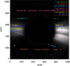 |
Fig. 1 Map of the tracks along the Metis UV field of view of the stellar targets used to infer the radiometric calibration factor ϵUV. The background UV image was acquired on January 16, 2021, at 12:31 UT. Image is in detector coordinates (in pixels). |
2.2 UVDA dark optimization
At the time of the radiometric calibration observations used in this work, the UV detector was subject to a “transient” effect that reduced the signal level of the images acquired in the first ~90 seconds after the command initiating the acquisition sequence. A description of this effect can be found in Andretta et al. (2021), Russano et al. (2024) and Uslenghi et al. (2024).
If single frames are acquired without the on-board co-adding step, the transient only affects the first few frames (which can be discarded during analysis). However, when on-board co-adding is employed to limit the data rate, the transient affects each group of images, leading to a complex alteration in the signal level of the resulting averaged image. This variation is dependent on several parameters, such as integration time, cadence, and the number of images averaged. Therefore, the acquisition of dark frames has been planned for each set of parameters used during science and calibration observations. Nevertheless, the transient also impacts the light signal, albeit to a lesser extent, introducing an additional uncertainty in photometric measurements. Thus, during the second part of the Cruise Phase, the on-board co-adding of frames was avoided.
In addition to the variations in the dark level caused by the transient issue, we observed small but significant (tens of DN) variations that appeared randomly, even over time scales of just a few hours. This resulted in dark frames acquired just a few hours later potentially failing to properly correct the science and/or calibration images. A detailed analysis revealed that these fluctuations are not consistent with pure offset or pure gain variations but rather with a linear combination of the two. Hence, if we have a dark frame (DF) measured at time t0, the dark frame at time t will be:
![Mathematical equation: $\[D F(t)=a(t) \cdot D F\left(t_0\right)+b(t).\]$](/articles/aa/full_html/2025/05/aa50759-24/aa50759-24-eq3.png) (1)
(1)
This is a purely empirical approach based on the study of dark frame sets acquired over long timescales. For dark images, the parameters a(t) and b(t) can be derived through a linear fit. To determine a(t) and b(t) for each non-dark image to be corrected, we utilized information contained within the images themselves; specifically, from the areas that are not illuminated by photons. In addition to the area behind the occulter, there are four corners not illuminated by the round fiber optics taper that connects the intensifier to the sensor (for a detailed description of the UV detector, see Antonucci et al. 2020b). By using the average values of boxes located in the non-illuminated areas of the detector, it was possible to compute the optimal dark subtraction for each calibration image. This was necessary due to the high nonuniformity of the sensor dark current, as these areas exhibit very different dark values. This allowed us to perform a fit with the Eq. (1) over five points. This algorithm has been validated on pairs of dark images.
The origin of these problems was identified and largely resolved through an upgrade to the on board software (OBSW) in April 2022.
2.3 Aperture photometry
Once the frames from the radiometric calibration observations were acquired and pre-processed with the steps described above, it was then possible to evaluate the star signal using the aperture photometry method, as previously done for the VL channel of Metis (De Leo et al. 2023). Briefly, the method consists in computing the signal measured over a circle of radius, r1, centered on the star after subtracting from it the corresponding background, proportionally calculated over an annular region with the same center, inner radius, r1 and outer radius, r2, as described by the equation:
![Mathematical equation: $\[C_{U V}=\sum_{i, j}^n S_{i j}-\frac{n}{m} \cdot \sum_{k, l}^m B_{k l}\]$](/articles/aa/full_html/2025/05/aa50759-24/aa50759-24-eq4.png) (2)
(2)
where Sij represents the signal per pixel within the circular area, Bkl is the background signal per pixel within the annular region, and n and m are the total number of pixels for the circle and the annulus, respectively. The conditions for {i, j} and {k, l} are given as: ![Mathematical equation: $\[\left\{i, j \mid \sqrt{\left(i-i_{0}\right)^{2}+\left(j-j_{0}\right)^{2}} \leq r_{1}\right\}\]$](/articles/aa/full_html/2025/05/aa50759-24/aa50759-24-eq5.png) and
and ![Mathematical equation: $\[\\left\{k, l \mid r_{1} \leq \sqrt{\left(k-i_{0}\right)^{2}+\left(l-j_{0}\right)^{2}} \leq r_{2}\right\}\]$](/articles/aa/full_html/2025/05/aa50759-24/aa50759-24-eq6.png) .
.
The best choice for the aperture radii r1 and r2 used for the background subtraction took into account the PSF of the instrument and the binning factor of the considered frame (when applicable). Considering that the full width half maximum (FWHM) of the Metis PSF ranges from 4 to 6.5 pixels throughout the FoV in the UV channel (Da Deppo et al. 2021), for our measurements, we chose a radius r1 of 12 pixels and r2 of 16 pixels. In case of data binned aboard, r1 and r2 have been divided by the binning factor of the frame. Fig. 2 shows the stellar flux growth as a function of the photometry aperture radius, r1. The variation in the star signal is about few percent for aperture radii larger than 10 pixels. We determined the error bars by propagating the error with the equation:
![Mathematical equation: $\[\sigma_{C_{U V}}=\sqrt{\sigma_S^2+2\left(n \cdot \sigma_B\right)^2}\]$](/articles/aa/full_html/2025/05/aa50759-24/aa50759-24-eq7.png) (3)
(3)
where σS is the statistical error associated with the star signal ![Mathematical equation: $\[\(\sim \sqrt{S})\]$](/articles/aa/full_html/2025/05/aa50759-24/aa50759-24-eq8.png) , n is the number of pixels of the circular area (depending on the value of r1), and σB is the standard deviation of the background signal values evaluated on the annular region. The count rate, NUV, differs from the integrated counts, CUV, only by the time exposure normalization of the frame in exam.
, n is the number of pixels of the circular area (depending on the value of r1), and σB is the standard deviation of the background signal values evaluated on the annular region. The count rate, NUV, differs from the integrated counts, CUV, only by the time exposure normalization of the frame in exam.
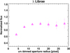 |
Fig. 2 Measured stellar flux of λ Librae as a function of the aperture radius r1 in pixels. The image was acquired on November 19, 2021, at 19:32 UT. |
2.4 Vignetting function correction
After the aperture photometry, we carried out another important step in the frame processing before proceeding with the calibration, which is the vignetting function (VF) correction. The FoVs of externally occulted coronagraphs are highly vignetted (see Fig. 3). Thus, a correction for the VF is required, to remove the artificial variation in the stellar flux along its track on the FoV. To this goal, for each frame used in this analysis, we divided the count rate, NUV, by the value of the vignetting function corresponding to the x and y-coordinates of the star centroid, VF (xstar, ystar). Considering that the VF values can vary over the pixel radius of the aperture photometry circle, we checked the difference of the count rate on one target, β 01 Scorpii, by performing the aperture photometry before and after the vignetting removal. The difference was found to be irrelevant.
The VF map used for the UV channel is the one measured for the VL channel during the on ground calibration campaign of the instrument (Antonucci et al. 2020b) and then corrected after the in-flight adjustment of the internal occulter (Liberatore et al. 2021). The VF map was also shifted to align its center with the in-flight center of the internal occulter (IO) and its size is rebinned in order to match that of the UV frame.
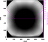 |
Fig. 3 Map of the VL vignetting function measured on-ground and adapted to the UV channel characteristics. The solid magenta line is the trend along the equatorial direction. Image is depicted in detector coordinates (in pixels). |
2.5 Metis UV photometric response
The Metis UV detector assembly (UVDA) consists of three main elements: (a) an intensifier, consisting of a micro channel plate (MCP) with KBr photocatode and a phosphor output screen, in optical contact with (b) a fiber optics 2:1 de-magnifying coupler connected to (c) a CMOS APS STAR1000 (1k × 1k format, 15 μm square pixel). The UVDA is installed at the end of the optical train consisting of the occulting sub-system, the telescope and the interferential filter assembly (IFA, Antonucci et al. 2020b; Fineschi et al. 2020). The IFA is an interferential Al/MgF2 multilayer filter deposited on a MgF2 crystal flat window. This element has the double purpose of selectively trans-mitting the H I Ly-α radiation to be detected by the UVDA, and of reflecting the visible light into the Metis VL channel. A High Voltage Unit (HVU) provides the high voltages required by the intensifier.
To determine the fluxes, f*, of the radiometric stellar targets in the UV narrow band, we calculated the results of the convolution of the UV spectra with the transmission curve of the interferential filter and the spectral response of the detector. In fact, the count rate, NUV, for each star is given via the equation:
![Mathematical equation: $\[\begin{aligned}N_{U V} & =\left[\int f_{*, \lambda} \cdot \epsilon_{F, \lambda} \cdot \epsilon_{U V D, \lambda} d \lambda\right] \cdot \epsilon_M{}^2 \cdot A_{p u p} \cdot V F~(\mathrm{FoV}) \\& =\left[\int f_{*, \lambda} \cdot \phi_F(\lambda) \cdot \phi_{U V D}(\lambda) ~d \lambda\right] \cdot \epsilon_{F, 121.6} \cdot \epsilon_{U V D, 121.6}. \\& \cdot \epsilon_M^2 \cdot A_{pup} \cdot V F~(\mathrm{FoV}) \\& =f_* \cdot \epsilon_{U V} \cdot A_{pup} \cdot V F~(\mathrm{FoV})\end{aligned}\]$](/articles/aa/full_html/2025/05/aa50759-24/aa50759-24-eq9.png) (4)
(4)
where f*,λ is the star spectrum, ϵF,λ = ϵF,121.6 · ϕF(λ) is the spectral profile of the filter transmission and ϕF(λ) the spectral profile normalized to the filter transmission at H I Ly-α121.6 nm, ϵUVD,λ = ϵUVD,121.6 · ϕUVD(λ) is the MCP spectral response and ϕUVD(λ) is the spectral profile normalized to the UVD quantum efficiency at H I Ly-α 121.6 nm (see Fig. 15 of Antonucci et al. 2020b), ϵM is the reflectivity of the telescope mirrors that can be assumed constant within the band pass, Apup is the telescope aperture, given by the external occulter stop, and VF (FoV) is the vignetting function, whose values depend on the position across the FoV.
The star spectra, f*,λ, in the UV band pass, can be observed only from space and come from the International Ultraviolet Explorer (IUE) experiment (Willis 2013), as well as from the SPectroscopy for the Investigation of the Characteristics of the Atmosphere of Mars (SPICAM) experiment (Bertaux et al. 2006). In Eq. (4), the Metis efficiency (or radiometric calibration factor) at H I Ly-α 121.6 nm is defined as
![Mathematical equation: $\[\epsilon_{U V}=\epsilon_{F, 121.6} \cdot \epsilon_{U V D, 121.6} \cdot \epsilon_M{}^2,\]$](/articles/aa/full_html/2025/05/aa50759-24/aa50759-24-eq10.png) (5)
(5)
and the star flux integrated in the UV pass band as
![Mathematical equation: $\[f_*=\int f_{*, \lambda} \cdot \phi_F(\lambda) \cdot \phi_{U V D}(\lambda) ~d \lambda.\]$](/articles/aa/full_html/2025/05/aa50759-24/aa50759-24-eq11.png) (6)
(6)
In Table 1, the values of the fluxes, f*, for each measured star, are reported with their errors dominated by the uncertainties on the stellar spectra, which (especially in the case of IUE data, in proximity of the H I Ly-α wavelength) can reach values of ~30%. The relative error on the detector response has a stable value of ~5% for the band pass and the relative error on the filter transmission is negligible. Fig. 4 shows some of the UV stellar spectra used in our analysis. Given the large and often unknown uncertainty in the stellar spectra data base we decided to uniformly weight the contribution of each star to the averaged ϵUV.
The radiometric calibration factor ϵUV (in DN/photon) is estimated by inverting the star signal NUV obtained from the aperture photometry, as follows:
![Mathematical equation: $\[\epsilon_{U V}(\mathrm{FoV})=\frac{N_{U V}~(\mathrm{FoV})}{f_* \cdot A_{p u p} \cdot V F~(\mathrm{FoV})}.\]$](/articles/aa/full_html/2025/05/aa50759-24/aa50759-24-eq12.png) (7)
(7)
In the ideal case (e.g., for the VL channel), the vignetting function correction removes completely the dependence of the star count rate on the position across the FoV, while the radiometric calibration factor maintains a constant value. As an example of our observations, Fig. 5 shows the signal of β 01 Scorpii along the FoV of the UV channel and the corresponding values of the vignetting function. The error bars in the figure are evaluated accordingly with the Eq. (3).
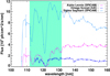 |
Fig. 4 Spectra of α Leonis, ω Scorpii and σ Sagittarii. The shaded area represents the UV narrow band of Metis, centered around 121.6 nm. Not all the spectra error bars are shown for clarity. |
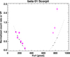 |
Fig. 5 Comparison between the normalized count rate (magenta diamonds) of β 01 Scorpii and the normalized VF (black dots). The VF is evaluated in the same positions of the star along the FoV. The black dashed line represents the continuous trend of VF. All trends have been normalized to the value of the first frame of this observation. In the figure, a discrepancy between the star signal and the VF trend is evident, on the east and the west sides of the UV FoV. The star signal error bars are multiplied by a factor 3 for clarity of the plot. The trend of the count rate corrected for the VF is shown in the first panel of Fig. 7. |
2.6 Correction for spatial disuniformity and data inversion
A discrepancy in the response is evident between the east side and the west side of the FoV. It reflects the fact that the radiometric factor remains dependent on the position across the FoV, after the vignetting function correction. This unexpected result has been extensively investigated and is present in all of the stars data analyzed. Thus, it is necessary to correct spatially the trend of the data to proceed with their inversion. By assuming that the ratio of brightness in the UV and VL closed-door frames is approximately constant across the FoV, the ratio between the images of both channels can provide an estimate of the map, MUV2VL (FoV), of the variation in the relative efficiency over the FoV. In the left panel of Fig. 6, we give an example of such a ratio. The procedure to derive the map MUV2VL (FoV), described in Appendix A. 2 of Andretta et al. (2021), is summarized in the following. A gradient in the azimuthal direction is evident in these ratios between UV and VL frames compared to the radial direction; some small-scale variations are nevertheless apparent which we believe are due to inhomogeneities in the reflectivity ratio of the door surface. To remove the effect of these small-scale inhomogeneities, we first averaged the UV-to-VL ratio maps over the radial direction; thus, we obtained a function of the azimuthal angle, which we then smoothed with a Gaussian filter with a standard deviation of 15 degrees. From this azimuthal, smoothed function, we then created the map MUV2VL (FoV) shown in the right panel of Fig. 6. This model is applied as an improvement of the standard UV vignetting function for every star of the data set. The map was normalized in a small square region of 65 × 65 pixels shown in Fig. 6. This area was originally selected for normalization because it is the region that was measured during the on ground calibration campaign and would make comparison between flight and ground calibration easier. The results from the ground calibration campaign are still under investigation and not discussed in this paper.
The four panels in Fig. 7 show a comparison between the count rates of β 01, ν, ω Scorpii, and 121 Tauri, corrected with the standard and spatially corrected VF. The error bars represent the propagated uncertainties, which account for the following factors: the uncertainty in the count rates, σNUV, in the vignetting function, σVF, and for spatially corrected data, the uncertainty in the spatial correction map, σMUV2VL. For the data that are not spatially corrected (blue triangles in Fig. 7), the uncertainty is calculated as:
![Mathematical equation: $\[\sigma_{\frac{N_{U V}}{V F}}=\frac{N_{U V}}{V F} \sqrt{\left(\frac{\sigma_{N_{U V}}}{N_{U V}}\right)^2+\left(\frac{\sigma_{V F}}{V F}\right)^2}.\]$](/articles/aa/full_html/2025/05/aa50759-24/aa50759-24-eq13.png) (8)
(8)
For the spatially corrected data (red triangles in Fig. 7), the uncertainty is determined as follows:
![Mathematical equation: $\[\sigma_{\frac{N_{U V}}{V F \cdot M_{U V2V L}}}=\frac{N_{U V}}{V F \cdot M_{U V 2 V L}} \sqrt{\left(\frac{\sigma_{N_{U V}}}{N_{U V}}\right)^2+\left(\frac{\sigma_{V F}}{V F}\right)^2+\left(\frac{\sigma_{M_{U V 2 V L}}}{M_{U V 2 V L}}\right)^2}.\]$](/articles/aa/full_html/2025/05/aa50759-24/aa50759-24-eq14.png) (9)
(9)
2.7 Refining the spatial correction across the FoV
With the goal of optimizing the spatial correction used above, we performed a statistical analysis of the obtained values of the radiometric calibration from each image of the star data set. First, we studied the spatial distribution of the absolute differences between the radiometric calibration factors (evaluated in the positions of each star within the detector frame) and the average radiometric calibration factor from the whole star data set. This distribution indicates a systematic trend. Then, to minimize it, we applied a linear correction to the UV-to-VL ratio map MUV2VL (FoV). Given the relatively few star points across the FoV, there are not enough constraints to attempt using a more complex surface. The linear correction was applied to the vertical direction only and was set to be equal to 1 in the region chosen for normalization. Thus, we simply wrote:
![Mathematical equation: $\[z=z_1+\frac{p \cdot\left(y-y_1\right)}{800}\]$](/articles/aa/full_html/2025/05/aa50759-24/aa50759-24-eq15.png) (10)
(10)
with z1 = 1.0 and y1 = 100 (the normalized box is centered on this y-coordinate). Eq. (10) depends on the p parameter, which represents how the fractionary correction of the plane applies to the stars count rates. Then we performed a least squares test on the differences between the values across the FoV and the average value. For every stellar target we summed the squared differences and we divided them for all the frames of that particular target, with the aim of finding the p parameter value that minimizes the test. This value is p = −0.24, that means the count rates with y-coordinate equal to 900 pixels have to be decreased by multiplying for a factor of 0.76.
Fig. 8 shows the least squares test results for the single stellar targets and for the entire data set (red squares) with respect to the p parameter. In the calculation of the global least squares test, we excluded four targets (β 01 Scorpii, θ Ophiuchi, τ Tauri, and 121 Tauri), whose data were affected by a large scatter from the beginning of the radiometric calibration procedure. Possible explanations of the data scatter are given in Appendix A.
Thus, we can write Eq. (7) as:
![Mathematical equation: $\[\epsilon_{U V}=\frac{N_{U V}~(\mathrm{FoV})}{f_* \cdot A_{p u p} \cdot V F~(\mathrm{FoV}) \cdot\left(M_{U V 2 V L}(\mathrm{FoV}) / z\right)}\]$](/articles/aa/full_html/2025/05/aa50759-24/aa50759-24-eq16.png) (11)
(11)
where MUV2VL (FoV) is the spatial correction map described in Sect. 2.6 and z the linear correction defined by Eq. (10). Fig. 9 shows the spatial correction map MUV2VL (FoV) divided by the linear correction z. With this additional linear correction, the spatial correction map MUV2VL (FoV)/z has now been optimized by removing a residual systematic spatial trend observed in the calibration coefficients of the individual stars.
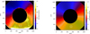 |
Fig. 6 Spatial correction map MUV2VL (FoV) modeled (right panel) by using the back-illuminated door frames (left panel). The white square indicates the normalization region. See the text for more details. The image is in detector (pixels) coordinates. |
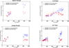 |
Fig. 7 Comparison between the star count rate corrected with the standard VF (blue triangles) and the count rates corrected with the spatially corrected VF (red triangles). The four stars of the panels are β 01, ν, ω Scorpii, and 121 Tauri. See the text for details. |
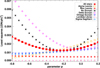 |
Fig. 8 Values of the least squares test with respect to the p parameter for each star and for the entire data set (red squares). See the text for details. |
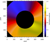 |
Fig. 9 UV-to-VL ratio after the application of the linear correction z: MUV2VL (FoV)/z. Image is in detector (pixels) coordinates. See the text for details. |
2.8 Final radiometric calibration results on the data set from June 2020 until December 2021
Figure 10 shows the results after performing all the corrections and the inversion of the data set, which consists of eleven stars. For each target we calculated the values of the radiometric calibration factor related to the position across the FoV, as a function of the radial distance from the center of the internal occulter. The error bars are derived from the error propagation on the Eq. (11), by taking into account all the sources of uncertainty involved in the inversion so far (e.g., errors on the count rate, on the star fluxes, on the VF and the spatial correction, etc.). Considering that the sample size is very different from one star to another, for each stellar target, we calculated the weighted average, to avoid the possibility that stars with larger number of frames could affect the estimate of the radiometric calibration coefficient. In Table 1 we reported the weighted average for each stellar target, without reporting the error which is affected mainly by the knowledge of the star flux. Therefore, in the final computation of the radiometric coefficient we consider each star contributing the same weight. The horizontal red solid line represents the ![Mathematical equation: $\[\bar{\epsilon}_{U V}\]$](/articles/aa/full_html/2025/05/aa50759-24/aa50759-24-eq17.png) value, estimated as the average of the star weighted averages from the whole data set. This value with the root mean square error (RMSE) 1σ is 0.20 ± 0.03.
value, estimated as the average of the star weighted averages from the whole data set. This value with the root mean square error (RMSE) 1σ is 0.20 ± 0.03.
The radiometric calibration presented here provides the average radiometric calibration factor, ![Mathematical equation: $\[\bar{\epsilon}_{U V}\]$](/articles/aa/full_html/2025/05/aa50759-24/aa50759-24-eq20.png) , and the refined spatial correction map, Mflight = MUV2VL (FoV)/z, to produce calibrated (L2) data.
, and the refined spatial correction map, Mflight = MUV2VL (FoV)/z, to produce calibrated (L2) data.
Finally, we checked if there was any trend of the radiometric calibration factor with time. The analyzed data set belongs to a time range, which spans through a year of the mission. For some targets, we have a double FoV transit; namely, 121 Tauri, with the first transit in January 2021 and the second one in August 2021, and θ Ophiuchi, with the first transit in March 2021 and the second one in December 2021. Fig. 11 shows the trend of the weighted average value, ϵUV,*, for every star with respect to time starting from June 2020 (the first month of the observations used for this work). The error bars are the weighted standard deviations, σ*, associated with the average value, ϵUV,*, for each stellar target. No changes in the average efficiency of the UV channel were observed until August 2021. The described analysis is extended until December 2021. In fact, there is no evidence of any degradation of the UV channel response; however, on the other hand, anomalies in the acquired frames were reported more frequently in the period between August and December 2021 (see the Appendix A).
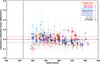 |
Fig. 10 Radiometric calibration factors as a function of the radial distance of the star images from the center of the occulter. The solid red line is the average value of |
![Mathematical equation: $\[\bar{\epsilon}_{U V}\]$](/articles/aa/full_html/2025/05/aa50759-24/aa50759-24-eq18.png)
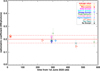 |
Fig. 11 Trend of the radiometric calibration factor ϵUV with respect to time, starting from June 2020 until August 2021. For every stellar target, the reported ϵUV is the weighted average value. The solid red line is the average value of |
![Mathematical equation: $\[\bar{\epsilon}_{U V}\]$](/articles/aa/full_html/2025/05/aa50759-24/aa50759-24-eq19.png)
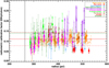 |
Fig. 12 Radiometric calibration factors as a function of the radial distance of the star images from the center of the occulter. The solid red line is the average value of |
![Mathematical equation: $\[\bar{\epsilon}_{U V}\]$](/articles/aa/full_html/2025/05/aa50759-24/aa50759-24-eq21.png)
2.9 State of the UV radiometric calibration after January 2022
As already mentioned, on January 2022 Metis suffered an automatic switch-off and the complete recovery of the instrument happened only three months later. The values of the applied high voltages (HV) to the camera were lowered, to increase safely margins in operating the UVD after the recovery. Thus, additional in-flight calibration campaigns are performed to verify that the overall response of the UV channel is in agreement with the prediction derived from the voltage change.
The calculation of ϵUV was carried out similarly to the procedure described in Sect. 2 of this work. We selected a data set of six stars, transiting the Metis FoV in the period July 2022 and July 2023: α and ρ Leonis, θ Ophiuchi, σ Sagittarii, π, and τ Scorpii. Only the latter two stars were observed for the first time, whereas all the other target observations were already used to perform the first evaluation of the radiometric calibration factor ϵUV (see Table 1).
As explained at the beginning of Sect. 2, the dark and bias signal is removed, then the images are corrected for the flat-field pattern. The star signal is retrieved by performing the aperture photometry (see Sect. 2.3) and transformed into count rates by dividing for the exposure time. After this, the count rates are divided by the VF value in the star centroid coordinates. To take into account the spatial disuniformity across the FoV, we applied the same correction described in Sect. 2.6, before inverting the star data. Figure 12 shows the results of the analysis just mentioned. For each stellar target, we determined the values of the radiometric calibration factor in the star positions across the FoV, as a function of the radial distance from the center of the internal occulter. Again, the error bars are obtained from the error propagation on the Eq. (11). The red solid line represents the average of the weighted averages of the stars and the red dashed lines depict the 1σ uncertainty evaluated as the RMSE of the data set. This value is 0.11 ± 0.03 and agrees within the error bars with the theoretical decrease of the radiometric calibration coefficient, due to the change in the voltages applied to the camera. During the radiometric campaign in 2020–2021 the MCP HV value was VMPC = 814 V, after the UVDA recovery is set to 900 V. The phosphor screen HV value passed from VS creen = 4545 V to 3484 V. Based on the HV change, the scaling factor of the UVDA response is about 68%, which produces a center value of 0.14 of the radiometric calibration coefficient (green solid line in Fig. 12). The UV data acquired after the recovery are calibrated with this preliminary value of the radiometric calibration factor, ϵUV, since January 2022 up to the time of writing. An analysis including a larger sample of stars and a thorough investigation of possible changes over time of the function, MUV2VL (FoV), is under way and will be the subject of a forthcoming publication.
3 Comparing radial UV profiles of Metis and UVCS
We compared the radial profiles of the H I Ly-α line intensity of Metis UV images obtained by applying the radiometric calibration described above with the profiles calculated using the archival data of UVCS. To perform this comparison, we analyzed the spectra obtained with UVCS and the images acquired with Metis, which were collected during the periods of minima of solar cycles 22 (in 1996) and 24 (in 2020–2021), respectively.
3.1 Radial profiles of UVCS
We considered a time interval of 6 months from April 1 to September 30, 1996 within the period of the solar minimum of cycle 22. For this period, we analyzed all the available observations (encompassing all heights) of the polar regions (±10° around the North and South Poles) and of the equatorial regions (±10° around the east and west limb). We selected the spectral region where the H I Ly-α was observed, and fit the spectrum with a function that corrects instrumental effects (Giordano, Ph.D. thesis, 1999) to determine the total intensity from each observed spectra. Then, analyzing for the same time interval all the observations of C III 977 and Si III 1206.5 spectral lines, which originate from the chromosphere and are not expected to be present in the hot corona, we removed the stray light contamination arising from the disk emission that may not have been completely suppressed by the occulters. Finally, we removed the H I Ly-α interplanetary (IP) contribution, estimated as ~3 × 10⁷ photons cm−2 s−1 sr−1, which is in agreement with values reported in previous studies (e.g., Kohl et al. 1997). As mentioned above, the emission in the polar regions is quite stable for a given heliocentric height, while in the equatorial regions, the modulation due to the passage of the active regions, which persist for more than one solar rotation, causes variations of almost an order of magnitude at some heights. Finally, by fitting the intensity as a function of distance with two different power-law functions, we obtained the equatorial and polar radial profiles shown in Fig. 13 (Giordano, in prep.) that can be compared with those observed with Metis.
3.2 Average radial profiles of Metis UV
Radial profiles of Metis images were extracted from level-2 data (L2, data release “V01”) by means of the following procedure. We first converted all images from Cartesian to polar (r, ϕ) coordinates determining a grid of polar coordinates. This grid had the axis of polar angle measured counterclockwise from the direction to the west solar equator with a step of 1° and the radial axis with a step, which depended on the distance of Metis to the Sun during different months and varied in the range from 0.02 to 0.09 R⊙. The H I Ly-α line intensity at each polar coordinate was estimated by means of a B-spline interpolation of order 1 (Briand & Monasse 2018) of the surrounding pixels of the original image. We calculated mean radial profiles for each polar angle ϕ using the data acquired with Metis during different months in 2020 and 2021 (see Table 2). Finally, we obtained equatorial and polar radial profiles of Metis averaging those of the polar regions (±10° around the northern and southern poles) and those of the equatorial regions (±10° around the western and eastern solar equators).
The resulting equatorial and polar radial profiles of Metis are shown in the top panels of Figs. 14 and 15, respectively. Bottom panels present the difference between the profiles obtained from Metis and UVCS observations. We also estimated the width of a distribution of the Metis data at each altitude, r, as its standard deviation. The obtained values are depicted by means of the shaded areas in Figs. 14 and 15 (bottom panels).
As Metis moves along its orbit, it performs observations from various distances to the Sun. This allows us to obtain and compare intensity profiles of the solar corona at various ranges of altitude; for instance, from 3.25–5.2 R⊙ on February 2021 to 5.6–9.4 R⊙ on November 2020. Even though the observations of UVCS have been carried out 25 years earlier than those of Metis, we found that equatorial intensity profiles of the two instruments are quite similar at heliocentric distances ≤ 6.5 R⊙. The difference of equatorial intensities between Metis and UVCS, which is typically lower than ~109 photons cm−2 s−1 sr−1, as well as the dispersion observed in the analyzed data can be caused by the activity level of the solar corona, the presence of bright stars in the field of view, and the occurence of coronal mass ejections (CMEs). At higher altitudes, average Metis profiles are also in a good agreement with that of UVCS extrapolated up to 9.4 R⊙.
During the solar minimum periods, there is a very low activity in the polar regions and the UV emission from the corona is low. At high heliocentric distances (>6 R⊙), where the density of coronal plasma is low and the wind speed is high, the H I Ly-α signal is expected to converge to the IP intensity. In these regions, the determination of the coronal signal is significantly challenged by the contamination of the IP background and the instrumental noise of Metis UV channel. We found that polar radial intensity profiles of Metis obtained for January, February, and August 2021 are consistent with UVCS profile at solar minimum and its extrapolation above 4.65 R⊙. The absolute difference of the corresponding intensities is typically lower than ~107 photons cm−2 s−1 sr−1. The intensity profiles calculated for November 2020, March and April 2021, which cover coronal heights from 4.5 to 9.4 R⊙, are a bit higher (by ~4 × 10⁷ photons cm−2 s−1 sr−1) than that obtained from the UVCS observations. Such a difference can be due to the presence of additional emission from the solar corona and/or a different level of IP emission observed during November 2020, March and April 2021. In fact, as measured with the Solar Wind ANisotropies (SWAN) experiment (Bertaux et al. 1995) on board SOHO, the IP intensity observed from ~1 au can range from 1.5 × 10⁷ to 8 × 10⁷ photons cm−2 s−1 sr−1, depending on the position of the instrument along the orbit around the Sun (see, e.g., Koutroumpa et al. 2017). However, we cannot exclude the presence of instrumental effects in the Metis UV channel (e.g., residual instrumental background or stray light) and/or UVCS data that can affect radiometric uncertainties in low coronal emission regions.
Finally, we would like to note that stars present in the FoV can alter the Metis profiles. For example, the pink profile in Fig. 15 has a peak at 4.7 R⊙ due to the passage of bright v and δ Scorpii on March 2021. In addition, stars passages increase a width of the distribution of the Metis data (see, e.g., pink profiles in the bottom panels of Figs. 14 and 15).
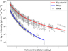 |
Fig. 13 H I Ly-α intensity profiles for polar and equatorial observations of UVCS at solar minimum. |
Metis UV data used for calculation of average radial profiles.
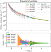 |
Fig. 14 Top panel: equatorial radial profiles of the H I Ly-α line intensity. Average Metis profiles obtained for different months are shown as green (November 2020), purple (January 2021), orange (February 2021), pink (March 2021), olive (April 2021) and cyan (August 2021) lines. UVCS data and intensity profile obtained for equatorial observations and summed with the contribution of the interplanetary H I Ly-α line intensity (IP, dotted line) are depicted as gray squares and red solid line, respectively. The dashed red line shows the extrapolation of the UVCS profile up to 9.5 R⊙ for comparison. Bottom panel: difference between the profiles of Metis and UVCS. The shaded areas represent the width of the distribution of Metis data (see text for details). |
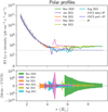 |
Fig. 15 Same as Fig. 14, but for polar radial profiles of Metis and UVCS. Top panel: UVCS data and intensity profile obtained for polar observations and summed with the contribution of the interplanetary H I Ly-α line intensity (IP, dotted line) are depicted as gray circles and blue solid line, respectively. The dashed blue line shows the extrapolation of the UVCS profile up to 9.5 R⊙ for comparison. Bottom panel: symmetrical logarithmic scale of the vertical axis for better visualization; i.e., it is logarithmic in both the negative and positive directions with a linear scale between −109 and 109 photons cm−2 s−1 sr−1. |
4 Conclusions
In this work, we present the results of the in-flight radiometric calibration of the UV channel of Metis coronagraph on board Solar Orbiter.
The radiometric calibration factor was obtained by using planned star observations in a time period from June 2020 until August 2021. After the vignetting function correction, it was necessary to perform additional corrections to address a significant non-uniformity in the spatial response across the FoV. This disuniformity was not adequately corrected by the VF determined during the on-ground characterization of the instrument visible light channel. The first correction corresponds to the spatial correction MUV2VL (FoV), obtained as the UV-to-VL ratio of the back-illuminated door frames, and the second one corresponds to a linear correction z, which optimizes such spatial correction by removing a residual systematic spatial trend observed in the calibration coefficients from the individual stars still remaining after multiplying VF by MUV2VL (FoV) (see Sects. 2.6 and 2.7). The value of the average radiometric calibration factor ![Mathematical equation: $\[\bar{\epsilon}_{U V}\]$](/articles/aa/full_html/2025/05/aa50759-24/aa50759-24-eq22.png) is equal to 0.20 ± 0.03 DN/photon. The radiometric calibration derived here (i.e., average calibration factor and refined spatial correction map Mflight = MUV2VL (FoV)/z) is used in the official pipeline of Metis, which produces calibrated (L2) data. We checked the trend with time of ϵUV, by exploiting repeated FoV transit of some stellar targets, and concluded that no degradation of the channel response has been observed (until August 2021). After the failure episode and the successful recovery of the UVDA, it was necessary to repeat the calculation of the radiometric calibration factor, ϵUV. Section 2.9 describes an up-to-date state of the UV channel radiometric calibration. An analysis of a larger sample of calibration stars that looks also at possible time variations of the MUV2VL (FoV) matrix is ongoing.
is equal to 0.20 ± 0.03 DN/photon. The radiometric calibration derived here (i.e., average calibration factor and refined spatial correction map Mflight = MUV2VL (FoV)/z) is used in the official pipeline of Metis, which produces calibrated (L2) data. We checked the trend with time of ϵUV, by exploiting repeated FoV transit of some stellar targets, and concluded that no degradation of the channel response has been observed (until August 2021). After the failure episode and the successful recovery of the UVDA, it was necessary to repeat the calculation of the radiometric calibration factor, ϵUV. Section 2.9 describes an up-to-date state of the UV channel radiometric calibration. An analysis of a larger sample of calibration stars that looks also at possible time variations of the MUV2VL (FoV) matrix is ongoing.
We compared average radial profiles of the H I Ly-α line intensity observed with UVCS and Metis during the periods of the activity minima of solar cycles 22 and 24, respectively. Although in our analysis we did not take into account systematic effects of solar origin (e.g. possible variability of the UV intensity from one solar cycle to another), we found that the resulting radial profiles are similar. The obtained agreement between the two instruments suggests that the contribution from the stray light and various anomalies (see Appendix A) to the UV data of Metis was (on average) quite moderate during the observations carried out up until August 2021. However, the 25-yr gap between the data sets of UVCS and Metis prevents us from deriving quantitative conclusions.
Acknowledgements
The authors thank the anonymous referee for the careful review, the constructive comments, and the support shown. Solar Orbiter is a space mission of international collaboration between ESA and NASA, operated by ESA. The Metis programme is supported by the Italian Space Agency (ASI) under the contracts to the cofinancing National Institute of Astrophysics (INAF): Accordi ASI-INAF No. I-043-10-0 and Addendum N. I-013-12-0/1, Accordo ASI-INAF No. 2018-30-HH.0 and under the contracts to the industrial partners OHB Italia SpA, Thales Alenia Space Italia SpA and ALTEC: ASI-TASI No. I-037-11-0 and ASI-ATI No. 2013-057-I.0. Metis was built with hardware contributions from Germany (Bundesministerium für Wirtschaft und Energie (BMWi) through the Deutsches Zentrum für Luft- und Raumfahrt e.V. (DLR)), from the Academy of Sciences of the Czech Republic (Czech PRODEX) and from ESA. Metis team thanks the former PI, Ester Antonucci, for leading the development of Metis until the final delivery to ESA. In this work we made use of the following open source and community-developed Python packages: Matplotlib (Hunter 2007), NumPy (Harris et al. 2020), SciPy (Virtanen et al. 2020), Astropy (Astropy Collaboration 2013, 2018, 2022) and SunPy (The SunPy Community 2020). Y.D.L. acknowledges support by Max-Planck-Institut für Sonnensystemforschung in Göttingen (Germany), the Università degli Studi di Catania (PIA.CE.RI. 2020–2022 Linea 2) and by the Italian MIUR-PRIN grant 2017APKP7T on “Circumterrestrial Environment: Impact of Sun-Earth Interaction”. P.H. was partially supported by the grant of the Czech Funding Agency No. 22-34841S and by the program “Excellence Initiative – Research University” for University of Wrocław, BPIDUB.4610.96.2021.KG.
Appendix A UVDA anomalies
Since the beginning of the analysis of the stars observations we noticed anomalies in the UVDA response, which made the in-flight radiometric calibration very challenging. The UV channel shows readout instabilities with non-linear variations both in the time and spatial domains.
The types of observed anomalies are different and in this section we summarize the ones which affect mostly the radiometric calibration frames. Other phenomenological descriptions of the anomalies can be found in Andretta et al. 2021, Russano et al. 2024, and Uslenghi et al. 2024. We already mentioned in Sect. 2.2 the problem related with the noticeable changes of the dark level from frame to frame at different time scales. As a consequence, calibration dark frames acquired with exactly the same detector parameters, do not always correct the UV frames. If appeared at short time scales, the effect is called “flickering.” This anomaly does not significantly affect the radiometric calibration results, because with the aperture photometry performed we subtract the image background to the star signal and thus the single image dark contribution is canceled. On the other hand, other images of Metis (i.e., the ones used for the comparison with UVCS data) are affected by this problem, thus the implemented procedure of dark normalization described in Sect. 2.2 was necessary.
We refer to another kind of anomaly as “flashes.” Episodically until August 2021, UV images of different data set showed an unexpected and sudden increase of the frame brightness. Left panel of Fig. 5 shows an example of this anomaly with the fourth and fifth values (magenta diamonds) of the count rate of β 01 Scorpii. These values are 50% larger than expected (black crosses), without any apparent explanation (i.e., changes in the acquisition parameters, transient events, etc.). These episodes are very rare in the frames of the data set and thus we decide to discard them.
Starting from August 2021, we noticed significant brightness variations in the UV Metis frames that are not consistent with the static background corona at the time of those observations. The behavior of the UVDA appeared to be bi-modal between two levels of brightness and affected entire data sets. We refer to these two values as “low state” and “high state” of the detector response. Fig. A.1 shows the λ Librae signal and the coronal background around the star with respect of time. Mostly from the background trend it is possible to see the bi-modal behavior of the UV channel response. The switch between the two levels was continuous and happened randomly. Furthermore, sometimes we noticed “halos” surrounding bright objects (i.e., stars, planets and prominences), when the detector was in a high state. The panels of Fig. A.2 show how the three conditions (low state, high state, high state with halos) of the detector response affect the frames of ζ 04 and λ Librae, observed in November 2021.
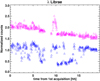 |
Fig. A.1 Star signal (magenta triangles) and coronal background (blue triangles) as a function of time for λ Librae. The star signal is shifted in the y-direction for clarity. The first image of the series was acquired on November 19, 2021, at 09:14 UT. |
The signal threshold variation affects also the data acquired after the UVDA recovery, but less severely. The origin of this effect is still under investigation.
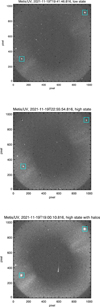 |
Fig. A.2 Three frames of the ζ 04 and λ Librae observation, happened in November 2021. ζ 04 Librae is the star on the top right of the detector, λ Librae is on the bottom left. The top panel depicts an example of “low state”, the middle panel depicts the “high state” and bottom panel a “high state” with “halos” surrounding the stars. The cyan squares highlight the area around the stars where the effect is visible. |
References
- Andretta, V., Bemporad, A., De Leo, Y., et al. 2021, A&A, 656, L14 [NASA ADS] [CrossRef] [EDP Sciences] [Google Scholar]
- Antonucci, E., Harra, L., Susino, R., & Telloni, D. 2020a, Space Sci. Rev., 216, 117 [CrossRef] [Google Scholar]
- Antonucci, E., Romoli, M., Andretta, V., et al. 2020b, A&A, 642, A10 [NASA ADS] [CrossRef] [EDP Sciences] [Google Scholar]
- Astropy Collaboration (Robitaille, T. P., et al.) 2013, A&A, 558, A33 [NASA ADS] [CrossRef] [EDP Sciences] [Google Scholar]
- Astropy Collaboration (Price-Whelan, A. M., et al.) 2018, AJ, 156, 123 [Google Scholar]
- Astropy Collaboration (Price-Whelan, A. M., et al.) 2022, ApJ, 935, 167 [NASA ADS] [CrossRef] [Google Scholar]
- Bertaux, J. L., Kyrölä, E., Quémerais, E., et al. 1995, Sol. Phys., 162, 403 [NASA ADS] [CrossRef] [Google Scholar]
- Bertaux, J.-L., Korablev, O., Perrier, S., et al. 2006, J. Geophys. Res. (Planets), 111, E10S90 [Google Scholar]
- Blackwell, D. E., & Petford, A. D. 1966, MNRAS, 131, 399 [NASA ADS] [CrossRef] [Google Scholar]
- Briand, T., & Monasse, P. 2018, Image Processing On Line, 8, 99 [CrossRef] [Google Scholar]
- Brueckner, G. E., Howard, R. A., Koomen, M. J., et al. 1995, Sol. Phys., 162, 357 [NASA ADS] [CrossRef] [Google Scholar]
- Colaninno, R. C., & Howard, R. A. 2015, Sol. Phys., 290, 997 [NASA ADS] [CrossRef] [Google Scholar]
- Da Deppo, V., Chioetto, P., Andretta, V., et al. 2021, SPIE Conf. Ser., 11852, 1185210 [Google Scholar]
- De Leo, Y., Burtovoi, A., Teriaca, L., et al. 2023, A&A, 676, A45 [NASA ADS] [CrossRef] [EDP Sciences] [Google Scholar]
- Domingo, V., Fleck, B., & Poland, A. I. 1995, Sol. Phys., 162, 1 [Google Scholar]
- Fineschi, S., Naletto, G., Romoli, M., et al. 2020, Exp. Astron., 49, 239 [Google Scholar]
- Focardi, M., Capobianco, G., Andretta, V., et al. 2014, SPIE Conf. Ser., 9144, 914409 [Google Scholar]
- Gabriel, A. H. 1971, Sol. Phys., 21, 392 [Google Scholar]
- Giordano, S., & Mancuso, S. 2008, ApJ, 688, 656 [NASA ADS] [CrossRef] [Google Scholar]
- Harris, C. R., Millman, K. J., van der Walt, S. J., et al. 2020, Nature, 585, 357 [NASA ADS] [CrossRef] [Google Scholar]
- Hunter, J. D. 2007, Comput. Sci. Eng., 9, 90 [NASA ADS] [CrossRef] [Google Scholar]
- Kaiser, M. L., Kucera, T. A., Davila, J. M., et al. 2008, Space Sci. Rev., 136, 5 [Google Scholar]
- Kohl, J. L., Esser, R., Gardner, L. D., et al. 1995, Sol. Phys., 162, 313 [Google Scholar]
- Kohl, J. L., Noci, G., Antonucci, E., et al. 1997, Sol. Phys., 175, 613 [Google Scholar]
- Koutroumpa, D., Quémerais, E., Katushkina, O., et al. 2017, A&A, 598, A12 [NASA ADS] [CrossRef] [EDP Sciences] [Google Scholar]
- Liberatore, A., Fineschi, S., Casti, M., et al. 2021, SPIE Conf. Ser., 11852, 1185248 [Google Scholar]
- Mihalas, D., & Binney, J. 1981, Galactic astronomy. Structure and kinematics (San Francisco: Freeman) [Google Scholar]
- Müller, D., St. Cyr, O. C., Zouganelis, I., et al. 2020, A&A, 642, A1 [Google Scholar]
- Noci, G., Kohl, J. L., & Withbroe, G. L. 1987, ApJ, 315, 706 [Google Scholar]
- Pence, W. D., Chiappetti, L., Page, C. G., Shaw, R. A., & Stobie, E. 2010, A&A, 524, A42 [NASA ADS] [CrossRef] [EDP Sciences] [Google Scholar]
- Romoli, M., Frazin, R. A., Kohl, J. L., et al. 2002, ISSI Sci. Rep. Ser., 2, 181 [NASA ADS] [Google Scholar]
- Romoli, M., Antonucci, E., Andretta, V., et al. 2021, A&A, 656, A32 [NASA ADS] [CrossRef] [EDP Sciences] [Google Scholar]
- Russano, G., Andretta, V., De Leo, Y., et al. 2024, A&A, 683, A191 [NASA ADS] [CrossRef] [EDP Sciences] [Google Scholar]
- Schühle, U., Teriaca, L., Aznar Cuadrado, R., et al. 2018, SPIE Conf. Ser., 10699, 1069934 [Google Scholar]
- Schwenn, R., Inhester, B., Plunkett, S. P., et al. 1997, Sol. Phys., 175, 667 [NASA ADS] [CrossRef] [Google Scholar]
- Thernisien, A. F., Morrill, J. S., Howard, R. A., & Wang, D. 2006, Sol. Phys., 233, 155 [NASA ADS] [CrossRef] [Google Scholar]
- The SunPy Community (Barnes, W. T., et al.) 2020, ApJ, 890, 68 [Google Scholar]
- Uslenghi, M., Schühle, U. H., Teriaca, L., Heerlein, K., & Werner, S. 2017, SPIE Conf. Ser., 10397, 103971K [NASA ADS] [Google Scholar]
- Uslenghi, M., Andretta, V., Teriaca, L., et al. 2024, SPIE Conf. Ser., 13103, 1310324 [Google Scholar]
- van de Hulst, H. C. 1950, Bull. Astron. Inst. Netherlands, 11, 135 [Google Scholar]
- Virtanen, P., Gommers, R., Oliphant, T. E., et al. 2020, Nat. Methods, 17, 261 [Google Scholar]
- Wenger, M., Ochsenbein, F., Egret, D., et al. 2000, A&AS, 143, 9 [NASA ADS] [CrossRef] [EDP Sciences] [Google Scholar]
- Willis, A. J. 2013, in Organizations, People and Strategies in Astronomy, 2, eds. A. Heck, 395 [Google Scholar]
- Withbroe, G. L., Kohl, J. L., Weiser, H., & Munro, R. H. 1982, Space Sci. Rev., 33, 17 [Google Scholar]
Level 1 (L1) data are uncalibrated (units of DN) and not corrected for any instrumental effect. On board binning (executed by averaging) is accounted for by storing in the data matrix the product of the counts to the number of binned pixels. In the case in which multiple frames are averaged on board, the data are also multiplied by the number of averaged frames.
The Flexible Image Transport System (FITS) header is updated to contain all the available orbital and attitude information, and image coordinates are given according to the FITS World Coordinate System (WCS, Pence et al. 2010, section 8). See also https://metis.oato. inaf.it/data_products.html
The flat-field matrices of Metis are 1024 × 1024 pixels arrays containing the normalized to unity small-scale (below 30 pixels in non-binned images) variations of the detector response. These variations are largely dominated by the gain pattern induced by the structure of the detector’s intensifier and, to a much smaller extent, by the pixel to pixel response variations of the Active Pixel Sensor (APS) coupled to it. The data used to build the flat-field matrix were acquired on ground with a quasi-flat illumination with a Ly-α source and a lens. There are 3 flat-field images, one for each possible binning of the Metis data (1×1, 2×2, 4×4).
All Tables
All Figures
|
Fig. 1 Map of the tracks along the Metis UV field of view of the stellar targets used to infer the radiometric calibration factor ϵUV. The background UV image was acquired on January 16, 2021, at 12:31 UT. Image is in detector coordinates (in pixels). |
| In the text | |
|
Fig. 2 Measured stellar flux of λ Librae as a function of the aperture radius r1 in pixels. The image was acquired on November 19, 2021, at 19:32 UT. |
| In the text | |
|
Fig. 3 Map of the VL vignetting function measured on-ground and adapted to the UV channel characteristics. The solid magenta line is the trend along the equatorial direction. Image is depicted in detector coordinates (in pixels). |
| In the text | |
|
Fig. 4 Spectra of α Leonis, ω Scorpii and σ Sagittarii. The shaded area represents the UV narrow band of Metis, centered around 121.6 nm. Not all the spectra error bars are shown for clarity. |
| In the text | |
|
Fig. 5 Comparison between the normalized count rate (magenta diamonds) of β 01 Scorpii and the normalized VF (black dots). The VF is evaluated in the same positions of the star along the FoV. The black dashed line represents the continuous trend of VF. All trends have been normalized to the value of the first frame of this observation. In the figure, a discrepancy between the star signal and the VF trend is evident, on the east and the west sides of the UV FoV. The star signal error bars are multiplied by a factor 3 for clarity of the plot. The trend of the count rate corrected for the VF is shown in the first panel of Fig. 7. |
| In the text | |
|
Fig. 6 Spatial correction map MUV2VL (FoV) modeled (right panel) by using the back-illuminated door frames (left panel). The white square indicates the normalization region. See the text for more details. The image is in detector (pixels) coordinates. |
| In the text | |
|
Fig. 7 Comparison between the star count rate corrected with the standard VF (blue triangles) and the count rates corrected with the spatially corrected VF (red triangles). The four stars of the panels are β 01, ν, ω Scorpii, and 121 Tauri. See the text for details. |
| In the text | |
|
Fig. 8 Values of the least squares test with respect to the p parameter for each star and for the entire data set (red squares). See the text for details. |
| In the text | |
|
Fig. 9 UV-to-VL ratio after the application of the linear correction z: MUV2VL (FoV)/z. Image is in detector (pixels) coordinates. See the text for details. |
| In the text | |
|
Fig. 10 Radiometric calibration factors as a function of the radial distance of the star images from the center of the occulter. The solid red line is the average value of |
| In the text | |
|
Fig. 11 Trend of the radiometric calibration factor ϵUV with respect to time, starting from June 2020 until August 2021. For every stellar target, the reported ϵUV is the weighted average value. The solid red line is the average value of |
| In the text | |
|
Fig. 12 Radiometric calibration factors as a function of the radial distance of the star images from the center of the occulter. The solid red line is the average value of |
| In the text | |
|
Fig. 13 H I Ly-α intensity profiles for polar and equatorial observations of UVCS at solar minimum. |
| In the text | |
|
Fig. 14 Top panel: equatorial radial profiles of the H I Ly-α line intensity. Average Metis profiles obtained for different months are shown as green (November 2020), purple (January 2021), orange (February 2021), pink (March 2021), olive (April 2021) and cyan (August 2021) lines. UVCS data and intensity profile obtained for equatorial observations and summed with the contribution of the interplanetary H I Ly-α line intensity (IP, dotted line) are depicted as gray squares and red solid line, respectively. The dashed red line shows the extrapolation of the UVCS profile up to 9.5 R⊙ for comparison. Bottom panel: difference between the profiles of Metis and UVCS. The shaded areas represent the width of the distribution of Metis data (see text for details). |
| In the text | |
|
Fig. 15 Same as Fig. 14, but for polar radial profiles of Metis and UVCS. Top panel: UVCS data and intensity profile obtained for polar observations and summed with the contribution of the interplanetary H I Ly-α line intensity (IP, dotted line) are depicted as gray circles and blue solid line, respectively. The dashed blue line shows the extrapolation of the UVCS profile up to 9.5 R⊙ for comparison. Bottom panel: symmetrical logarithmic scale of the vertical axis for better visualization; i.e., it is logarithmic in both the negative and positive directions with a linear scale between −109 and 109 photons cm−2 s−1 sr−1. |
| In the text | |
|
Fig. A.1 Star signal (magenta triangles) and coronal background (blue triangles) as a function of time for λ Librae. The star signal is shifted in the y-direction for clarity. The first image of the series was acquired on November 19, 2021, at 09:14 UT. |
| In the text | |
|
Fig. A.2 Three frames of the ζ 04 and λ Librae observation, happened in November 2021. ζ 04 Librae is the star on the top right of the detector, λ Librae is on the bottom left. The top panel depicts an example of “low state”, the middle panel depicts the “high state” and bottom panel a “high state” with “halos” surrounding the stars. The cyan squares highlight the area around the stars where the effect is visible. |
| In the text | |
Current usage metrics show cumulative count of Article Views (full-text article views including HTML views, PDF and ePub downloads, according to the available data) and Abstracts Views on Vision4Press platform.
Data correspond to usage on the plateform after 2015. The current usage metrics is available 48-96 hours after online publication and is updated daily on week days.
Initial download of the metrics may take a while.