| Issue |
A&A
Volume 696, April 2025
|
|
|---|---|---|
| Article Number | L21 | |
| Number of page(s) | 3 | |
| Section | Letters to the Editor | |
| DOI | https://doi.org/10.1051/0004-6361/202554745 | |
| Published online | 29 April 2025 | |
Letter to the Editor
Kolmogorov analysis of JWST deep survey galaxies
1
National Research Nuclear University MEPhI, Moscow, Russia
2
Center for Cosmology and Astrophysics, Alikhanian National Laboratory and Yerevan State University, Yerevan, Armenia
3
School of Physics and Astronomy, Monash University, Clayton, Australia
4
SIA, Sapienza University of Rome, Rome, Italy
⋆ Corresponding author: This email address is being protected from spambots. You need JavaScript enabled to view it.
Received:
25
March
2025
Accepted:
16
April
2025
Abstract
JWST galaxy deep spectral surveys provide a unique opportunity to trace a broad range of evolutionary features of galaxies and the intergalactic medium given the huge distance the photons are propagating. We have analyzed the spectral data of JWST galaxies up to a redshift of around 7 using the Kolmogorov technique, which is an efficient tool for testing the tiny comparative randomness properties of cumulative signals, that is, for distinguishing the contributions of regular and stochastic sub-signals. Our aim is to determine if certain identical spectral features of galaxies have undergone any distortions or systematic evolution across a broad range of redshifts. Our results indicate a change in the spectral properties of the sample galaxies at around z ≃ 2.7 at over a 99% confidence level.
Key words: galaxies: high-redshift
© The Authors 2025
 Open Access article, published by EDP Sciences, under the terms of the Creative Commons Attribution License (https://creativecommons.org/licenses/by/4.0), which permits unrestricted use, distribution, and reproduction in any medium, provided the original work is properly cited.
This article is published in open access under the Subscribe to Open model. This email address is being protected from spambots. You need JavaScript enabled to view it. to support open access publication.
1. Introduction
The data produced by JWST on the high-redshift Universe reveal remarkable features regarding early galaxies, star formation, supermassive black holes, and numerous associated aspects (see Cooper et al. 2025; D’Silva et al. 2025; Liu et al. 2025; Martis et al. 2025; Runnholm et al. 2025; Sun et al. 2025; Pérez-González et al. 2025 and references therein). Certain observational data are seen to challenge the predictions of the standard cosmological model, or at least call for the reconsideration of particular issues. Various data analysis techniques, including those involving artificial intelligence and machine learning (Robertson et al. 2022), are being used to study the ever-increasing amount of high-redshift observational data.
We analyzed JWST spectral data of galaxies up to redshift z ≃ 7. We employed the Kolmogorov stochasticity parameter (KSP) approach (Kolmogorov 1933; Arnold 2008a,b) to analyze the comparative features of the spectral signals of the galaxies. The KSP is an efficient tool for studying the comparative randomness features of cumulative signals and dynamical systems (Arnold 2008b, 2009a,b; Atto et al. 2013). Namely, the KSP enables signals to be distinguished based on their composition of regular and random sub-signals, and can thus be applied to physical signals with regular components and foreground stochastic noise. Regarding astrophysical signals, the KSP test has been applied in studies of non-Gaussianities in cosmic microwave background (CMB) data (Gurzadyan & Kocharyan 2008; Gurzadyan et al. 2009). In particular, the KSP enabled Gurzadyan et al. (2014) to draw conclusions regarding the void nature of the Cold Spot in the CMB Planck sky map; soon after that study, a void aligned with the Cold Spot was detected in an infrared galactic survey (Szapudi et al. 2015). The dynamical difference of structures at local and global cosmological scales can lead to different observational signals (Gurzadyan & Stepanian 2021; Gurzadyan et al. 2023, 2025). The difference in the KSP properties enabled the CMB signal to be clearly distinguished from the microwave emission of the Galactic disk (Gurzadyan & Kocharyan 2008; Gurzadyan et al. 2009); this revealed XMM-Newton X-ray galaxy clusters (Gurzadyan et al. 2011) and gamma sources (Gurzadyan et al. 2010), confirming the efficiency of the approach for a broad class of physical issues.
We used the KSP test to determine if there are any signal distortions or redshift-dependent variations for JWST galaxies across a broad range of redshifts.
2. Kolmogorov stochasticity parameter
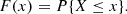
Arnold (2008a,b, 2009a,b) outlined the remarkable efficiency of Kolmogorov’s theorem (Kolmogorov 1933) in defining the randomness properties of real-valued sequences. Consider a {X1, X2, …, Xn} sequence of n random variables X ordered in an increasing manner, X1 ≤ X2 ≤ … ≤ Xn, and its cumulative distribution function (CDF):
 (1)
(1)
One can define an empirical distribution function as
Then, the KSP λn is defined as
 (2)
(2)
Kolmogorov (1933) proved that, for any continuous CDF,
where Φ(0) = 0,
 (3)
(3)
this limit converges uniformly, and Kolmogorov’s distribution, Φ, is independent of the CDF. It can be shown that, within 0.3 ≤ λn ≤ 2.4, the KSP acts as an objective degree of randomness (Arnold 2008a,b). These features of the Kolmogorov distribution make the KSP test an efficient tool for analyzing the comparative randomness properties of signals.
3. Dataset
The galaxy spectroscopic data of the JWST NIRSpec instrument (McElwain et al. 2023; Jakobsen et al. 2022) from the Ultradeep NIRSpec and NIRCam Observations before the Epoch of Reionization (UNCOVER) survey (Price et al. 2024; Bezanson et al. 2024) allow spectral signals from the observed galaxies to be inspected across a broad range of redshifts.
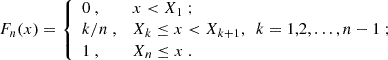
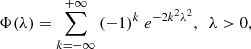
Price et al. (2024) divided galaxies by their redshift fit quality and we performed a KSP analysis of the signals for spectra with redshift quality flags “secure” and “solid”. Galaxies with a maximum spectrum corresponding to a wavelength nearly equal to 656 [nm] in the rest frame were selected for the analysis. They cover a broad range of redshifts, 1.86 ≤ z ≤ 7.05, and contain the majority of data points for the sample, including 148 galaxies. Figure 1 shows the dependence of the wavelength corresponding to the maximum spectrum on the redshift of the galaxies.
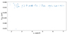 |
Fig. 1. Dependence of the wavelength on the redshift of the galaxies’ spectral maxima in the rest frame. |
The procedure described in Sect. 2 was performed on the abovementioned wavelength sequence of the galaxies.
4. Analysis
We performed a KSP analysis on these galaxy spectral data. To obtain the KSP dependence of the signal at a given redshift, the following procedure was adopted. One thousand nonidentical pairs of uniformly distributed numbers corresponding to redshifts z1 < z2 were generated such that each z1 < z2 interval contained 10–20 galaxies. Then, the KSP was calculated within those interval samples (i.e.,  ), enabling us to assign a degree of randomness to a given redshift. We note that although the number of galaxies within the selected redshift intervals is small, the KSP test remains efficient as an indicator of randomness; its capability to detect such characteristics has previously been demonstrated for small data sequences (Arnold 2008a).
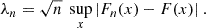
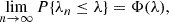
To estimate the KSP, the wavelength values in each interval were normalized to the mean value (0) and the variance (1). Normalization enables a generalized normal distribution to be used as the theoretical distribution, with a single free parameter representing the sharpness of the distribution. The generalized normal distribution with variance equal to 1 was taken as the theoretical distribution. Figure 2 shows the dependence of the KSP value on the redshift in this scheme and its comparison with the KSP of the mock data of the same distribution. To illustrate the scale of deviation of the KSP of the real data from that of the generated distribution sample, the  dependence on z is plotted in Fig. 3, where Δλ is the difference between the mean values of the KSP and σλ is the standard deviation of the mock data KSP. The plot shows that the deviation reaches a level of 4σ.
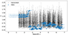 |
Fig. 2. Redshift dependence of the KSP λ of the galaxy emission corresponding to the maximum of the spectrum. Blue points denote the KSP values calculated for the observed galaxies, and horizontal error bars indicate the selected [z1; z2] intervals. Black points indicate the median of the mock data KSP, and the vertical error bars are the 99% confidence intervals around the medians of the generated data. |
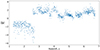 |
Fig. 3. Redshift dependence of the scale of deviation of the KSP value from the generated distribution. |
The resulting dependence in Fig. 2 was smoothed using a moving average with a redshift window of Δz = 0.1 to provide a more robust evaluation of the deviation level. Figure 4 shows the averaged KSP values (with a 99% confidence interval) of the generated distribution. A change in the KSP values is evident at z ≃ 2.7.
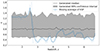 |
Fig. 4. Moving average of Fig. 2 with window Δz = 0.1. Blue points are the averaged values, and the error bars are the standard deviations of the points inside the window. The black line denotes the averaged median KSP of the generated distribution, and the shaded region is the 99% confidence interval around the median. |
5. Conclusions
We have analyzed JWST deep galaxy spectral survey data by means of the Kolmogorov technique. The Kolmogorov stochastic parameter has been shown (Arnold 2008a,b) to enable comparisons of the tiny randomness properties of cumulative signals, that is, signals composed of regular and random (stochastic) sub-signals. We analyzed the spectral data of the JWST galaxy survey up to redshift z ≃ 7 to KSP-test whether the data of the same survey keep certain properties independent of the redshift, or if they undergo distortions or evolve. Thus, it is crucial that the instrumental noise and certain systematics are identical for the galaxies of the dataset.
The results of the KSP analysis show a change in the JWST galaxy spectral properties at z ≃ 2.7, at over a 99% confidence level. Namely, the results indicate a change in the random and regular components of a given galactic signal at a certain redshift, that is, the appearance or disappearance of certain agents contributing to that spectral signal at that redshift. The nature of this effect can be related to the features of the galaxy evolution and/or to the properties of the intergalactic medium through which the photon beams are propagating, linked with, for example, galactic dark haloes (De Paolis et al. 2014) and their broad extensions (Mistele et al. 2024), or an invisible population of galaxies (Varnish et al. 2025). Therefore, studying the revealed galactic spectral signature variation at certain redshifts by other means and using other data samples within broad redshift intervals can shed light on its nature.
Acknowledgments
We are thankful to the referee for valuable comments. We acknowledge the use of NASA/ESA/CSA James Webb Space Telescope data obtained from the Mikulski Archive for Space Telescopes at the Space Telescope Science Institute.
References
- Arnold, V. I. 2008a, Nonlinearity, 21, T109 [Google Scholar]
- Arnold, V. I. 2008b, Uspekhi Mat. Nauk, 63, 5 [CrossRef] [Google Scholar]
- Arnold, V. I. 2009a, Trans. Moscow Math. Soc., 70, 31 [CrossRef] [Google Scholar]
- Arnold, V. I. 2009b, Funct. An. Other Math., 2, 139 [Google Scholar]
- Atto, A. M., Berthoumieu, Y., & Megret, R. 2013, Entropy, 15, 4782 [Google Scholar]
- Bezanson, R., Labbe, I., Whitaker, K. E., et al. 2024, ApJ, 974, 92 [NASA ADS] [CrossRef] [Google Scholar]
- Cooper, R. A., Caputi, K. I., Iani, E., et al. 2025, arXiv e-prints [arXiv:2502.18310] [Google Scholar]
- De Paolis, F., Gurzadyan, V. G., Nucita, A. A., et al. 2014, A&A, 565, L3 [NASA ADS] [CrossRef] [EDP Sciences] [Google Scholar]
- D’Silva, J. C. J., Driver, S. P., Lagos, C. D. P., et al. 2025, arXiv e-prints [arXiv:2503.03431] [Google Scholar]
- Gurzadyan, V. G., & Kocharyan, A. A. 2008, A&A, 492, L33 [NASA ADS] [CrossRef] [EDP Sciences] [Google Scholar]
- Gurzadyan, V. G., & Stepanian, A. 2021, A&A, 653, A145 [NASA ADS] [CrossRef] [EDP Sciences] [Google Scholar]
- Gurzadyan, V. G., Allahverdyan, A. E., Ghahramanyan, T., et al. 2009, A&A, 497, 343 [NASA ADS] [CrossRef] [EDP Sciences] [Google Scholar]
- Gurzadyan, V. G., Kashin, A. L., Khachatryan, H. G., et al. 2010, EPL, 91, 19001 [Google Scholar]
- Gurzadyan, V. G., Durret, F., Ghahramanyan, T., et al. 2011, EPL, 95, 69001 [Google Scholar]
- Gurzadyan, V. G., Kashin, A. L., Khachatryan, H. G., et al. 2014, A&A, 566, A135 [NASA ADS] [CrossRef] [EDP Sciences] [Google Scholar]
- Gurzadyan, V. G., Fimin, N. N., & Chechetkin, V. M. 2023, A&A, 677, A161 [NASA ADS] [CrossRef] [EDP Sciences] [Google Scholar]
- Gurzadyan, V. G., Fimin, N. N., & Chechetkin, V. M. 2025, A&A, 694, A252 [NASA ADS] [CrossRef] [EDP Sciences] [Google Scholar]
- Jakobsen, P., Ferruit, P., Alves de Oliveira, C., et al. 2022, A&A, 661, A80 [NASA ADS] [CrossRef] [EDP Sciences] [Google Scholar]
- Kolmogorov, A. N. 1933, G. Ist. Ital. Attuari, 4, 83 [Google Scholar]
- Liu, F. Y., Dunlop, J. S., McLure, R. J., et al. 2025, arXiv e-prints [arXiv:2503.07774] [Google Scholar]
- Martis, N., Withers, S., Felicioni, G., et al. 2025, arXiv e-prints [arXiv:2503.01579] [Google Scholar]
- McElwain, M. W., Feinberg, L. D., Perrin, M. D., et al. 2023, Publ. Astron. Soc. Pac., 135, 058001 [Google Scholar]
- Mistele, T., McGaugh, A., Lelli, F., et al. 2024, ApJ, 969, L3 [NASA ADS] [CrossRef] [Google Scholar]
- Pérez-González, P. G., Östlin, G., Costantin, L., et al. 2025, arXiv e-prints [arXiv:2503.15594] [Google Scholar]
- Price, S. H., Bezanson, R., Labbe, I., et al. 2024, arXiv e-prints [arXiv:2408.03920] [Google Scholar]
- Robertson, B. E., Tacchella, S., Johnson, B. D., et al. 2022, ApJ, 942, L42 [Google Scholar]
- Runnholm, A., Hayes, M. J., Mehta, V., et al. 2025, arXiv e-prints [arXiv:2502.19174] [Google Scholar]
- Sun, F., Fudamoto, Y., Lin, X., et al. 2025, arXiv e-prints [arXiv:2503.15587] [Google Scholar]
- Szapudi, I., Kovacs, A., Granett, B. G., et al. 2015, MNRAS, 450, 11 [Google Scholar]
- Varnish, T. W. O., Wu, X., Pearson, C., et al. 2025, MNRAS, 539, 347 [Google Scholar]
All Figures
|
Fig. 1. Dependence of the wavelength on the redshift of the galaxies’ spectral maxima in the rest frame. |
| In the text | |
|
Fig. 2. Redshift dependence of the KSP λ of the galaxy emission corresponding to the maximum of the spectrum. Blue points denote the KSP values calculated for the observed galaxies, and horizontal error bars indicate the selected [z1; z2] intervals. Black points indicate the median of the mock data KSP, and the vertical error bars are the 99% confidence intervals around the medians of the generated data. |
| In the text | |
|
Fig. 3. Redshift dependence of the scale of deviation of the KSP value from the generated distribution. |
| In the text | |
|
Fig. 4. Moving average of Fig. 2 with window Δz = 0.1. Blue points are the averaged values, and the error bars are the standard deviations of the points inside the window. The black line denotes the averaged median KSP of the generated distribution, and the shaded region is the 99% confidence interval around the median. |
| In the text | |
Current usage metrics show cumulative count of Article Views (full-text article views including HTML views, PDF and ePub downloads, according to the available data) and Abstracts Views on Vision4Press platform.
Data correspond to usage on the plateform after 2015. The current usage metrics is available 48-96 hours after online publication and is updated daily on week days.
Initial download of the metrics may take a while.