| Issue |
A&A
Volume 696, April 2025
|
|
|---|---|---|
| Article Number | A145 | |
| Number of page(s) | 21 | |
| Section | Cosmology (including clusters of galaxies) | |
| DOI | https://doi.org/10.1051/0004-6361/202554232 | |
| Published online | 11 April 2025 | |
Interference in fuzzy dark matter filaments
Idealized models and statistics
1
Institute of Theoretical Astrophysics, University of Oslo, PO Box 1029, Blindern, 0315 Oslo, Norway
2
Theoretical Particle Physics and Cosmology, King’s College London, Strand, London WC2R 2LS, UK
3
Department of Physics, Imperial College London, Blackett Laboratory, Prince Consort Road, London SW7 2AZ, UK
4
Dunlap Institute for Astronomy and Astrophysics, University of Toronto, 50 St. George St., Toronto, ON M5S 3H4, Canada
⋆ Corresponding author; This email address is being protected from spambots. You need JavaScript enabled to view it.
Received:
23
February
2025
Accepted:
6
March
2025
Abstract
Fuzzy (wave) dark matter (FDM), the dynamical model underlying an ultralight bosonic dark matter species, produces a rich set of nongravitational signatures that distinguishes it markedly from the phenomenologically related warm (particle) dark matter (WDM) scenario. The emergence of extended interference fringes hosted by cosmic filaments is one such phenomenon reported by cosmological simulations, and a detailed understanding of such may strengthen existing limits on the boson mass but also break the degeneracy with WDM, and provide a unique fingerprint of interference in cosmology. In this paper, we provide initial steps toward this goal. In particular, we show in a bottom-up approach, how the presence of interference in an idealized filament population can lead to a non-suppressive feature in the matter power spectrum – an observation supported by cosmological FDM simulations. To this end, we build on a theoretically motivated and numerically observed steady-state approximation for filaments and express the equilibrium dynamics of such in an expansion of FDM eigenstates. We optimize the size of the expansion by incorporating classical phase-space information. Ellipsoidal collapse considerations were used to construct a fuzzy filament mass function which, together with the reconstructed FDM wave function, allowed us to efficiently compute the one-filament power spectrum. We showcase our non-perturbative interference model for a selection of boson masses and confirm our approach is able to produce the matter power boost observed in fully cosmological FDM simulations. More precisely, we find an excess in correlation between the spatial scale associated with the FDM ground state and the quantum pressure scale. We speculate about applications of this effect in data analysis.
Key words: methods: numerical / methods: statistical / dark matter / large-scale structure of Universe
© The Authors 2025
 Open Access article, published by EDP Sciences, under the terms of the Creative Commons Attribution License (https://creativecommons.org/licenses/by/4.0), which permits unrestricted use, distribution, and reproduction in any medium, provided the original work is properly cited.
This article is published in open access under the Subscribe to Open model. This email address is being protected from spambots. You need JavaScript enabled to view it. to support open access publication.
1. Introduction
If the observed dark matter (DM) in the Universe (Planck Collaboration VI 2020) is bosonic and has a sufficiently low mass, m ≲ 1 eV, then it can be modeled as a classical wave on astrophysical scales. For definiteness, we consider a scalar (or pseudoscalar) field. The gravitational physics of a scalar field is distinct from a gas of cold, pressureless particles, that is, cold DM (CDM). Scalar fields obey the Klein-Gordon equation, while CDM obeys the collisionless Boltzmann equation. If the particle mass is sufficiently low, m ≲ 10−18 eV, then the distinction between wave-like DM and CDM can show up on cosmological scales. Since the effect of DM waves is typically to smooth out structures relative to CDM, such a model is referred to as “fuzzy” DM (FDM, see e.g., Hu et al. 2000; Marsh & Silk 2014; Marsh 2016; Hui et al. 2017).
If all the DM is to be fuzzy, then its mass is bounded from below to be m ≳ 10−21 − 10−19 eV with the weaker limit coming from Milky Way satellite galaxy population statistics and their internal structure (Nadler et al. 2019; Zimmermann et al. 2024), and the stronger limit coming from dynamics of star clusters in ultrafaint dwarf galaxies (Marsh & Niemeyer 2019; Dalal & Kravtsov 2022). An array of limits populates the parameter space in between (Iršič et al. 2017; Kobayashi et al. 2017; Armengaud et al. 2017; Nori et al. 2019; Nadler et al. 2019; Rogers & Peiris 2021; Banik et al. 2021; Powell et al. 2023). FDM of lower-mass 10−32 eV ≲ m ≲ 10−24 eV is restricted to be a subdominant component of the DM making up at most 20% of the total mass density (Hlozek et al. 2015, 2018; Kobayashi et al. 2017; Laguë et al. 2022; Dentler et al. 2022; Rogers et al. 2023; Winch et al. 2024). The prevalence of such ultralight particles in high energy physics models (Arvanitaki et al. 2010; Mehta et al. 2021; Cicoli et al. 2022; Sheridan et al. 2024), together with their potential of alleviating tensions between cosmological and astrophysical probes (Rogers et al. 2023; Rogers & Poulin 2025), encourages the search for cosmological evidence of FDM across the entire allowed parameter space.
The wave-like nature of FDM leads to a number of physical effects distinct from CDM ((Marsh et al. 2023)), including the existence of a Jeans scale (Khlopov et al. 1985), the formation of solitons (Schive et al. 2014; Levkov et al. 2018), and turbulence leading to relaxation (Hui et al. 2017), and all of these effects have been exploited in efforts to constrain and search for FDM. However, there is no more canonical signature of a particle being a wave than the presence of interference fringes. In fully cosmological simulations of FDM, interference fringes are observed in a striking way inside cosmic filaments (Schive et al. 2014; Mocz et al. 2019; May & Springel 2023). As noted by Mocz et al. (2019), the presence of such interference is a distinctive feature of FDM that distinguishes it markedly from the related warm DM (WDM) model: both WDM and FDM suppress structure growth on small spatial scales, but only FDM introduces interference patterns that modulate the density on scales comparable to the (reduced) de Broglie-wavelength λdB = ℏ/(mv) (Hui et al. 2017).
Filaments are particularly intriguing structures in the context of constraining the nature of DM. Particle DM simulations with and without suppressed initial conditions suggest filaments realize a volume filling fraction of ∼20% for z > 3, while maintaining a fairly constant mass filling fraction of ≳50% (Dome et al. 2023b). Weak gravitational lensing is an ideal probe for detecting this filamentary DM density (Mead et al. 2010) and observational advances using this detection method are encouraging (Xia et al. 2020; HyeongHan et al. 2024). Lyman-alpha (Lyα) emission from neutral hydrogen (H I) tracing DM is another detection mechanism and future observational facilities, such as the Extremely Large Telescope, may be equipped to reveal Lyα emitting filamentary structures of the cosmic web (Liu et al. 2024). Lyα absorption, more precisely the spectrally resolved forest of absorption lines, has proven to be an indispensable probe for the small-scale behavior of DM (e.g., Viel et al. 2005; Rogers & Peiris 2021; Rogers et al. 2022; Iršič 2024). Its flux power spectrum arises from low H I column density regions, tracing less nonlinear DM overdensities < 10 (Lukić et al. 2015) common for void-like regions and filament outskirts. Returning to Fig. 1, we find this region to be strongly modulated by interference. In this work, we concretely assess whether the scales on which interference manifests in filaments are above or below the pressure filtering scale of the intergalactic medium that sources the Lyα forest and thus is relevant for these analyses.
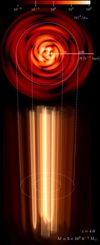 |
Fig. 1. Top: Cross section of a steady-state FDM filament with FDM mass m = 2 × 10⁻²² eV at redshift z = 4. The interference is constructed as a post-processing step for an interference-free background density which may be provided by an analytical model (this work) or DM simulations (future work). Bottom: Volume rendering of a toy filament obtained by extruding above cross section along a straight filament spine. Section 2 models FDM filaments as infinitely long versions of such extrusions. In Sect. 3 we find a physically-sound extrusion length for our 2D model via ellipsoidal collapse considerations. |
In the context of FDM, we note that in comparison to halos, filaments are less compact objects, with shallower gravitational wells and thus have smaller characteristic velocities (Mocz et al. 2019). As wave effects manifest around the de Broglie scale with coherence time t ∼ λdB/v, interference features at fixed mass are expected to be more pronounced and less transient compared to highly nonlinear halos – an expectation supported by simulation (Mocz et al. 2019; May & Springel 2023).
Providing a more principled, theoretical understanding of interference in cosmic filaments is thus a timely contribution with the ultimate aim to provide a large-scale structure, interference-only DM mass limit. In this paper we focus on (i) the construction of a simplified model for FDM interference in filaments and (ii) the question of how to measure interference features statistically.
Fully nonlinear simulations of the nonrelativistic limit of Klein-Gordon – the Schrödinger-Poisson equation (SP) – are challenging (Schive et al. 2014; Mocz et al. 2019; May & Springel 2021, 2023; Laguë et al. 2024) and approximate treatments remain crucial to forward model isolated elements of the FDM phenomenology. If one is interested in large-scale morphological changes of a fuzzy cosmic web and its constituents, encoding FDM’s suppression physics in the initial conditions, but treating it dynamically as CDM, has proven effective (Dome et al. 2023a,b). Combining this “classical FDM” approximation with emulation techniques (Rogers et al. 2019; Rogers & Peiris 2021) enabled Rogers & Peiris (2021) to derive m > 2 × 10⁻²⁰ eV due to a lack of structure suppression in the Lyα forest. The emergence of solitonic cores and their relation to its environment, on the other hand, may be faithfully reproduced by an approximate hydrodynamic formulation of SP (Mocz & Succi 2015; Nori & Baldi 2018, 2021). However, none of these approximate methods are able to produce interference. The approximate Gaussian beams method is exceptional in that it can produce interference (Schwabe & Niemeyer 2022), but it has not been deployed in large studies. An intriguing alternative to these SP-simulation-based approaches is a physically-informed post-processing of non-FDM data. Put simply, in the context of filaments, we seek a self-consistent prescription for “painting on interference fringes” on CDM filaments. This work makes initial steps toward this goal.
Building upon advances in the steady-state modeling of spherically symmetric FDM halos (Lin et al. 2018; Yavetz et al. 2022; Zimmermann et al. 2024), we confine ourselves to isothermal, steady-state filaments (Stodólkiewicz 1963; Ostriker 1964; Ramsøy et al. 2021). We translate the spherically symmetric halo prescription to cylindrical filaments and further develop the model by incorporating classical phase-space information.
Fully-fledged SP simulations also provide guidance on how interference is expected to manifest quantitatively. More precisely, Mocz et al. (2019), May & Springel (2021, 2023) independently report a boost in the matter power spectrum at scales k ≥ 𝒪(100) h Mpc−1, compared to the smoothed WDM spectrum and ultimately the CDM case at z ≤ 7. Quite intuitively, it was conjectured that this feature may be related to interference fringes on scales above the quantum pressure scale. Anticipating our result, we show in a proof-of-concept analysis that our idealized filament model is indeed able to produce interference fringes in accordance with these scales and leading to the power boost fully nonlinear simulations suggest.
The paper is organized as follows: Sect. 2 develops and showcases our idealized toy model for FDM interference. Sect. 3 investigates statistical aspects of a fuzzy filament population and, in particular, its population statistics (i.e., a FDM filament mass function) as well as two-point density correlation (i.e., the matter power spectrum). We discuss our findings in Sect. 4. Conclusions are drawn in Sect. 5.
2. An idealized model for interference in cosmic filaments
The point of departure is a discussion of our idealized, semi-analytical model for interference in FDM filaments – an extension of the regression approach developed in Yavetz et al. (2022) by a physically-informed prior based on a steady-state phase space information (Widrow & Kaiser 1993; Lin et al. 2018; Dalal et al. 2021). We refer to Fig. 1 for a preview.
After introducing interference reconstruction in a general setting in Sect. 2.1, we specialize to the case of steady-state filaments in Sect. 2.2. To this end, we develop a self-consistent description of quasi-virial filaments in both real space, Sect. 2.2.1, and phase space, Sect. 2.2.2. Specifics of our modified regression approach are outlined in Sect. 2.3. We close by showcasing our model for a range of relevant FDM masses and phase space model parameters in Sect. 2.4.
2.1. Self-consistent FDM interference in steady-state systems
In the nonrelativistic limit applicable for the study of cosmic structure formation, FDM is governed by the Schrödinger-Poisson equation (e.g., Hui 2021). With m denoting the FDM mass, a(t) the scale factor, and G as Newton’s constant, the Schrödinger-Poisson equation reads as follows:
![Mathematical equation: $$ \begin{aligned} i\hbar \partial _t\psi&=\left[- \frac{\hbar ^2}{2m a^2(t)}\mathop \!\mathbin \bigtriangleup + mV(\boldsymbol{x}, t) \right]\psi , \end{aligned} $$](/articles/aa/full_html/2025/04/aa54232-25/aa54232-25-eq1.gif) (1a)
(1a)
 (1b)
(1b)
We note that ψ ∈ ℂ represents the FDM field, commonly dubbed the wave function, which is self-consistently coupled to its own gravitational potential V via Poisson’s equation. |ψ|2 measures the FDM density in a comoving volume. For the remainder of this paper comoving coordinate components are denoted with capital letters while physical components are lower case, for example, x = (R, Φ, Z) for comoving and r = (r, ϕ, z) physical cylindrical coordinates.
Equation (1a), a nonlinear Schrödinger equation with explicitly time-dependent Hamiltonian, is challenging in its numerical treatment as all physically relevant scales – from Mpc-sized filaments down to the de-Broglie scale inside halos ( with σ2 as characteristic halo velocity dispersion) need to be resolved in order to guarantee convergence and stability (Schive et al. 2014; Garny et al. 2020; May & Springel 2021).
Fortunately, if one is only interested in a self-consistent treatment of interference effects in isolated objects, it is possible to forego a fully-fledged integration of Eqs. (1a)–(1b) under the assumption that the detailed dynamics encapsulated in ψ(x, t) take place in a smooth gravitational potential that is effectively static in time (Lin et al. 2018; Dalal et al. 2021).
A canonical example where this holds true is a virialized DM halo. Violent relaxation and phase mixing (Lynden-Bell 1967) drive collisionless CDM into a virial equilibrium with universal Navarro-Frenk-White (NFW) density profiles (Navarro et al. 1996). The associated relaxation time scale may be approximated with the free fall time,  (Lynden-Bell 1967), and is characteristic for changes in the potential due to out-of-equilibrium density configurations. Similarly, FDM halos realize NFW-like densities comprised of short-lived interference granules with coherence time (Hui et al. 2021):
 (2)
(2)
This large-scale equivalence to CDM is a consequence of the Schrödinger-Vlasov correspondence (Uhlemann et al. 2014; Mocz et al. 2018) and it is only at small radii where gravitational Bose-Einstein condensation (Levkov et al. 2018) causes a deviation due the formation of a solitonic core (Schive et al. 2014).
For mean halo densities of 200 times the background matter density,  , we find tc ≪ trel ≪ tH ≈ (Gρm)−1/2. Consequently, one expects the gravitational potential to appear roughly static on the dynamical time scale of the interference evolution and approximately maintained on the time scale of the expanding background. The latter implies that the scale factor can be treated as fixed. We note that the halo density and potential enjoy approximate spherical symmetry.
We investigate how similar conditions, that is, a quasi-static gravitational potential with a high degree of symmetry may be justified in a limiting case of cosmic filaments in Sect. 2.2.
With a time-independent, interference-free potential in place Eqs. (1a)–(1b) reduce to:
![Mathematical equation: $$ \begin{aligned} i\hbar \partial _t\psi&=\left[- \frac{\hbar ^2}{2m a^2}\mathop \!\mathbin \bigtriangleup + mV(\boldsymbol{x}) \right]\psi ,\end{aligned} $$](/articles/aa/full_html/2025/04/aa54232-25/aa54232-25-eq7.gif) (3a)
(3a)
 (3b)
(3b)
and Eq. (3b) is solved only once to fix the time-independent Hamiltonian. Importantly, Eq. (3a) is decoupled from Eq. (3b) and no nonlinearity is present. We may interpret this system of PDEs as the linear order perturbative treatment of interference with V as zeroth-order potential (Dalal et al. 2021).
Integrating Eq. (3a) in time reduces to diagonalizing its Hamiltonian and expanding ψ(x, t) in the eigenbasis {ψj(x)}j = 1…J with energy eigenvalues {Ej}j = 1…J. The time evolution is thus set by:
 (4)
(4)
and the sought-after interference emerges as the cross-terms in the time-dependent density:
 (5)
(5)
Self-consistency requires us to find complex coefficients aj such that the time-independent term in Eq. (5) recovers the static background density ρBG(x), that is:
 (6)
(6)
A few remarks are in order. Firstly, Eq. (6) only fixes the coefficient moduli, but leaves the phases ωj unspecified. We follow Yavetz et al. (2022) and sample ωj ∼ U([0,2π)). ⟨|ψ|2⟩ thus denotes the expectation value over all phases.
Secondly, a direct comparison between solution of Eqs. (3a)–(3b) and Eqs. (1a)–(1b) for virialized halos show satisfying agreement (Yavetz et al. 2022).
Thirdly, although the requirement Eq. (6) implies that each eigenstate must obey the same symmetries as the steady-state background – spherical for halos, cylindrical for filaments –|ψ(x, t)|2, and in particular the interference term in Eq. (5), does not. As shown in Fig. 1, interference fringe features beyond the assumed symmetry in ρBG can thus be realized.
Finally, despite our focus on FDM interference, there is no a priori reason to restrict ourselves to FDM-only steady-state background models. As shown in Yavetz et al. (2022), as long as the set of eigenstates is able to reproduce all properties of ρBG on the spatial scales of interest (in this work > 1 kpc), the latter is a viable input to the interference model. This opens up the possibility to use the above model prescription as a post-processing tool for CDM simulations of steady-state objects, an intriguing application we leave to a future work.
To apply the outlined procedure to the case of FDM filaments, three ingredients are required: (i) a background density model (ii) a library of eigenstates and eigenenergies and (iii) a procedure to satisfy Eq. (6). We address each point in Sects. 2.2 and 2.3.
2.2. FDM filaments as infinitely long, isothermal cylinders
Let us map the general discussion of Sect. 2.1 to the special case of fuzzy filaments with the goal to establish Eqs. (3a)–(3b) as a viable approximation to Eqs. (1a)–(1b).
From the onset, we stress that there is no a priori reason to expect that the entire cosmic filament population may be attributed with universal properties like a complete relaxation into virial equilibrium or a NFW-profile analog. Even from an idealized theoretical viewpoint (Zel’dovich 1970; Bond & Myers 1996), filaments represent only partially collapsed objects, still expanding or contracting along their spines on a time scale comparable to the Hubble time, tH, ultimately turning into fully collapsed, virialized halos. This is no different for FDM structure formation and an enlightening volume rendering of this process is shown in Nori & Baldi (2021).
To complicate matters, simulations suggest that a variety of factors may determine the physical conditions and morphology of a filament, most notably spatial scale (e.g., Colberg et al. 2005), cosmic environment (Ramsøy et al. 2021), and properties of DM (Mocz et al. 2019; May & Springel 2023). In light of this physically diverse filament population and our aim to establish a time-independent, linear approximation akin to Eq. (1a), we distinguish between two limiting cases based on the kinematic state: bulk-flow-dominated and quasi-virialized filaments.
Bulk-flow dominated filaments (e.g., Odekon et al. 2022) represent > 𝒪(1 Mpc) structures acting as accretion channels for DM and gas into the gravitational well of the adjacent DM halos. Their radial density structure is consistent with a broken power-law profile with a power law index γ = −2 in the outskirts (Colberg et al. 2005; Dolag et al. 2006; Aragón-Calvo et al. 2010; Zhu et al. 2021) and core regions consistent with −1 ≤ γ ≤ 0. It is clear that Eqs. (3a)–(3b) can not be a bona fide description of this filament population as the impact of the environment, in particular inflow and outflow of matter is excluded: ψ and its steady-state density ρBG model an isolated, self-gravitating object. We return to the question of how one may model bulk-flow dominated filaments in Sect. 5.
The quasi-virialized case (Stodólkiewicz 1963; Ostriker 1964), by contrast, constitutes a theoretically idealized scenario in which filaments are approximated locally by an infinitely long, isothermal, cylinder. In it each cross section attained a steady-state, virial equilibrium and dynamics along the longitudinal direction are suppressed. The model is appealing as (i) it maps well to the assumptions leading to Eqs. (3a)–(3b) and (ii) the derivation of the steady-state real-space density ρBG and even its phase space distribution is tractable. We clarify these aspects in Sects. 2.2.1 and 2.2.2.
Interestingly, recent high-resolution simulations of intermediate-size (≲𝒪(1) Mpc) CDM filaments around Milky Way-like progenitors (Ramsøy et al. 2021) are able to reproduce filaments of this type – a statement found to be true across redshifts z = 3 − 8. Moreover, Eisenstein et al. (1997) propose to estimate the dynamical mass of large scale filaments under isothermal cylinder conditions and find the approximation to work reasonably well when compared against N-body simulations.
The remainder of this work focuses on the wave function reconstruction in the quasi-virial limit as well as observable changes in statistical measures due to the presence of interference sourced by such filaments, cf. Sect. 3. Dynamical implications of interference (Dalal & Kravtsov 2022) will not be considered. This allows us to construct the interference field in Eq. (5) at only one instance of cosmic time t and thus at a frozen scale factor value a = a(t). We choose z = 4 to be (i) within the applicability region of the isothermal cylinder approximation (Ramsøy et al. 2021), (ii) near the regime in which the large scale behavior of the FDM power spectrum is dominantly determined by the choice of initial conditions (May & Springel 2023) (thereby simplifying the construction of the filament mass function in Sect. 3.1), and (iii) compatible with the results of of Gough & Uhlemann (2024), with which we make contact in Sect. 4.
2.2.1. Real space density
We first argue that the interference contained in the full wave function has negligible impact on the gravitational potential. For this, we posit that filaments may be approximated as isolated, infinitely long, at this stage not necessarily isothermal, cylinders. Consequently, the right hand side of Eq. (1b) reduces to |ψ|2, which is, by assumption, now constant along the filament spine. The gravitational potential for a non-axially symmetric source |ψ(x)|2 = |ψ(R, Φ)|2 reads:
 (7)
(7)
with G(x, x′) = (2π)−1log(|x − x′|) denoting the free-space Greens function in polar coordinates. Compared to a canonical 1/r-kernel in spherical symmetry, a log-potential shows strong smoothing properties when used in the convolution of Eq. (7), effectively rendering the interference contribution in |ψ|2 to the total gravitational potential subdominant.
Let us illustrate this smoothing effect based on the strongly oscillating wave function shown in Fig. 1. For this, we compare the potential produced by the non-axially symmetric, interference-modulated density |ψ|2, with the axial-symmetric interference-free contribution ⟨|ψ|2⟩. For each contribution we compute the gravitational potential according to Eq. (7) (Hejlesen et al. 2019) and compare their relative importance in Fig. 2.
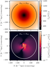 |
Fig. 2. Top: Gravitational potential sourced by the axial-symmetric contribution ⟨|ψ|2⟩Φ = ⟨|ψ|2⟩ of the wave function depicted in Fig. 1. Bottom: Relative importance of the potential perturbation sourced by the interference term alone. Neglecting the latter in the computation of the total potential in Eq. (1b) only incurs 𝒪(1 − 10%) errors. |
Evidently, the interference part of the wave function induces small, mostly per-cent level, changes to the total gravitational potential sourced by |ψ|2. Thus, we may substitute |ψ|2 → ⟨|ψ|2⟩ in Eq. (7) and only incur a relatively small error in the potential.
Next, we seek for an axial-symmetric filament background density ρBG(R) that may replace the wave function all together and thus removes the nonlinear coupling between Schrödinger’s and Poisson’s equation.
On scales larger than λdB the Schrödinger-Vlassov correspondence (Uhlemann et al. 2014; Mocz et al. 2018) allows us to treat FDM as collisionless particles. In accordance with our introductory remarks, let the behavior of these particles be described by a velocity dispersion tensor of the form:
and thus neglecting longitudinal dynamics, ⟨vz⟩=⟨vz2⟩ = 0, and bulk rotation, ⟨vϕ⟩ = 0. Isothermal conditions are imposed by assuming the radial moment, ⟨vr2⟩, azimuthal moment, ⟨vϕ2⟩, and consequently the anisotropy parameter,
 (8)
(8)
are constant throughout the filament.
Starting from the cylindrical Jeans equation (Binney & Tremaine 2008) and above dispersion tensor, Eisenstein et al. (1997) derive closed form, analytic solutions for the density ρ and its associated line density μ(r):1
 (9)
(9)
 (10)
(10)
r0 denotes the transition scale between the small radii, ρ ∼ r−β, and large radii behavior, ρ ∼ rβ − 4. In contrast to an NFW profile or the isothermal sphere, the integrated (line) mass μ remains finite as r → ∞:
 (11)
(11)
We call filaments defined as above “quasi-virial” since the relation between total line mass μ, dispersion σ2 and anisotropy parameter β is a direct consequence of the tensor virial theorem applied to the infinite cylinder geometry. The isotropic, β = 0, derivation is given in Fiege & Pudritz (2000).
As noted earlier, Ramsøy et al. (2021) find intermediate-sized CDM filaments in Milky Way sized progenitor halos to adhere to the isotropic profile in Eq. (9)2. More precisely, their filament sample is consistent with a quasi-static evolution of Eq. (9) between redshift z = 3 − 8, that is, the functional form of the density profile remains valid throughout this redshift bin and only a time dependence in the velocity dispersion σ2 → σ2(a) and scale radius r0 → r0(a) is introduced. For reference, at redshift z* = 4 one finds r0(a*)≃10 kpc and  (Ramsøy et al. 2021).
It is interesting to note that, although the forgoing discussion assumed collisionless dynamics, by virtue of the large-scale equivalence of CDM and FDM, a stability analysis (Desjacques et al. 2018) suggests that Eq. (9) is a stable density configuration for SP3.
May & Springel (2023) extract radial filament density profiles for CDM and FDM from a comparable set of cosmological simulations and find both populations to have cuspy inner densities at z = 3. We may realize such cuspy profiles by assuming a radially biased velocity anisotropy, that is, β > 0.
We thus arrive at the sought-after, axial-symmetric, comoving background density ρBG:
 (12)
(12)
It is this density that sources the potential within which the filament wave function evolves.
2.2.2. Phase space distribution function
With a background density, Eq. (12), in place we ask what the associated phase space distribution function (DF) looks like. Constructing the latter for generic axial-symmetric systems, for instance, galactic disks, is a daunting task, both theoretically (Hunter & Qian 1993) and numerically (Petač & Ullio 2019) – especially in the case of prolate objects (Merritt 1996) like finite extend filaments.
Fortunately, in the case of infinitely long cylinders, c.f. Sect. 2.2.1, the situation simplifies drastically and is conceptionally close to the situation found for spherically symmetric but anisotropic systems (Binney & Tremaine 2008).
According to Jeans’ theorem, we may assume that a steady-state DF is a function of three isolating integrals of motion only. In the case of a classical particle moving in the gravitational potential sourced by an infinitely long cylinder, these are trivially identified as the specific energy contribution of both the longitudinal, Ez, and transversal motion, E, as well as the specific angular momentum L:
 (13)
(13)
where ui ≡ pi/m denote the velocities associated with the momenta conjugate to comoving coordinates, that is,  and L as effective Lagrange function of a classical particle in an expanding universe (Peebles 1980; Bartelmann 2015). We remind the reader that the scale factor is fixed and energy is therefore a conserved quantity.
Jeans’ theorem then suggests the DF ansatz:4
 (14)
(14)
and μ as defined in Eq. (11). Marginalizing over velocity space provides us with the radial density implied by the DF of Eq. (14):
 (15)
(15)
We wish to invert this expression to obtain f(E, |L|). However, Eq. (15) is ill-defined without further restrictions on the angular momentum dependence of f as different radial velocity dispersions can in principle realize the same radial density profile. In accordance with Sect. 2.2.1, we break this degeneracy by enforcing a constant anisotropy β. Either through direct computation or by application of the augmented density formalism (Dejonghe 1986), we find:
 (16)
(16)
to guarantee β = const. The yet to be determined function g(E) then follows by demanding that marginalizing Eq. (16) recovers the background density of Eq. (12). We set ρDF(R) = ρBG(R) in Eq. (15) and perform the uΦ-integration to arrive at:
![Mathematical equation: $$ \begin{aligned} \rho _\text{BG}(R) = 2 a^2\sqrt{\pi } \frac{\Gamma \left(\frac{1-\beta }{2}\right)}{\Gamma \left(\frac{2-\beta }{2}\right)} R^{-\beta } \int \limits _{V(R)}^{\infty } \!\mathrm{d} E \frac{g(E)}{\left[2a^2(E-V(R))\right]^{\beta /2}}, \end{aligned} $$](/articles/aa/full_html/2025/04/aa54232-25/aa54232-25-eq25.gif) (17)
(17)
with β ∈ ( − ∞, 1). For the physically relevant range of anisotropies β ∈ [0, 1), Eq. (17) is equivalent to an Abel integral equation and thus existence of a solution for g(E) is guaranteed5.
This concludes the construction of the background model. In summary, in the limit of quasi-virial filaments, it is possible to find a self-consistent description in real and phase space. We use ρBG in Eq. (12) to find the gravitational potential V via Eq. (19b) and use the density-potential pair as input to the inverse problem of Eq. (17), the solution of which gives us access to the DF.
We refer to Fig. 3 for an illustration of the density, both from Eqs. (12) and (17) for two values of the anisotropy parameter β. The correspondence between both profiles is satisfying, and therefore demonstrates the effectiveness of our numerical inversion for Eq. (17), the solution of which is depicted in Fig. 4. For both choices of β, the inversion converges to a DF that is exponential in the specific energy E.
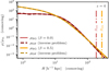 |
Fig. 3. Radial filament densities obtained from Eq. (12) (solid lines) and the solution of the inverse problem of Eq. (17) (dashed lines), i.e., the density implied by the DF. Vertical lines depict the fit radius R99 within which 99% of the total line mass μ are contained. |
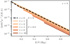 |
Fig. 4. Recovered DFs for the densities depicted in Fig. 3 for various values of the specific angular momentum L = l × ℏm−1. Note that (i) we only show L = 0 for β = 0 as the DF is uniform in L for isotropic conditions, cf. Eq. (16), (ii) energies are bound from below by Ec(L), the energy of a circular orbit defined as the minimum of the effective potential V(R)+L2/2a2R2 and (iii) both DFs recover a Boltzmann-like, exponential behavior in E. We emphasize that this functional behavior is not imposed by our inversion of Eq. (17). |
2.2.3. Eigenstate library
We may realize an infinitely long, cylindrical geometry by solving Eqs. (3a)–(3b) in a domain unbound in X, Y-direction and periodic in Z. A factorization of the eigenmode ψj(x) into:
 (18)
(18)
 (19a)
(19a)
 (19b)
(19b)
with radial eigenstates  and n ∈ ℕ, l ∈ ℤ as radial (number of nodes of Rnl) and angular quantum number respectively. The Hamiltonian is symmetric in l. Consequently, the specific energy eigenvalues satisfy En, −l = Enl as well as Rn, −l(R) = Rnl(R) and we may restrict the construction of the library to positive angular momenta.
The numerical treatment of Eq. (19a) is more challenging than the spherically symmetric halo case, in part because of the form the angular momentum barrier takes, see Appendix A for a discussion.
For a fixed value of l, the radial eigenstates of Eq. (19a) are found by a Chebyshev pseudospectral discretization that respects the parity properties of the modes ψj(x) in Eq. (18) (Lewis & Bellan 1990; Trefethen 2000). This results in a dense matrix representation of the Hamiltonian, Hl, for which we compute the eigensystem and retain all modes with Enl ≤ V(R99). R99 corresponds to the radius within which 99% of the total line mass μBG are contained and the stated inequality discards all eigenstates with a classically allowed region larger than our fiducial fit radius Rfit = R99. The procedure is repeated for increasing values of l until the minimum of the effective potential, Veff, ψ, surpasses our cutoff energy V(R99). Note that this procedure does not set the number of eigenstates, Jl, a priori, but finds all modes up to the cutoff energy as long as the spatial discretization satisfies rank(Hl) > Jl. We depict a library excerpt for m = 2 × 10⁻²² eV and an isotropic background density at redshift z = 4 in Fig. 5.
Depending on input parameters {z, m, β} a complete eigenstate library contains 𝒪(102)−𝒪(104) modes (and consequently the same number of mode coefficients aj ∈ ℂ). Thus, we end up with a highly flexible model potentially prone to overfitting. Section 2.3 outlines how the DF constructed in Sect. 2.2.2 may be used to arrive at a minimal model that still recovers the steady-state density ρBG as closely as possible.
2.3. Wave function reconstruction
Under cylindrical symmetry and ansatz Eq. (19a), the self-consistency condition, Eq. (6), is recast to:
 (20)
(20)
There exist multiple approaches for computing the coefficients anl. Widrow & Kaiser (1993) propose a physically-intuitive procedure and set the coefficients according to the DF – after all |anl|2 may be interpreted as the probability of finding state |ψnl|2 and the value of the DF represents the classical probability of a system state with energy Enl and angular momentum Lnl. In the cylindrical case considered here it is therefore natural to assume:
 (21)
(21)
Lin et al. (2018), Dalal et al. (2021) show the effectiveness of this approach in the case of virialized, fully isotropic halos for which the DF is a function of energy only. More precisely, Eq. (21) produces FDM halos closely following an NFW halo upon time or phase averaging. However, deviations are found at small radii. An explanation for this behavior is given by Yavetz et al. (2022): Eq. (21) is only correct in the WKB-limit of high energies E ≫ V. Hence, only these modes are assigned correct coefficients. Since highly excited eigenstates have broader spatial extent, cf. Fig. 5, they dominate the mode composition in the halo outskirts and produce the correct density profile. Low energy eigenstates, on the other hand, don’t contribute to the outskirt density and their poorly chosen coefficients only contribute to deviations in the core region.
 |
Fig. 5. Subset of the eigenstate library for m = 2 × 10⁻²² eV and β = 0 at redshift z = 4. The total library for this parameter combination contains J = 746 states. As is the case for halos, the small radii behavior of radial eigenstates is determined by the angular momentum Rnl(R)∼Rl, while n ∈ ℕ is equivalent to the number of nodes in Rnl. For fixed l, the maximal n is set by Enl < V(R99) and lmax follows from min(Veff, ψ) < V(R99). |
Appendix B derives the high energy WKB correspondence between DF and the wave function coefficients for the case of infinitely long filaments of line mass μ. One finds:
 (22)
(22)
where Lnl represents an effective mapping from quantum number l to the classical, specific angular momentum L. Its form is motivated by Langer’s correction (Langer 1937) and modified at l = 0 where anisotropic DFs diverge, cf. Eq (16). We fix the constant L0 < 1 such that a wave function with coefficients set according to Eq. (22) reproduces the background density ρBG up to R ∼ 1 kpc.
For this we turn to Fig. 6 illustrating the effectiveness of the WKB assignment scheme in the case of quasi-virialized filaments. Under isotropic conditions (top panel) the DF is independent of L rendering the choice of L0 irrelevant. For β > 0 (lower panel), an ad hoc value of L0 = 0.1 recovers the cuspy density profile reasonably well up to R ∼ 1 kpc.
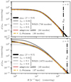 |
Fig. 6. Comparison of various coefficient estimators |anl|2 for m = 2 × 10⁻²² eV with β = 0 (top) and β = 0.5 (bottom) at z = 4. While the WKB result, Eq. (22), reproduces the background density well without any optimization, the posterior modes adaptive LASSO and l1-Poisson show identical accuracy while reducing the number of involved modes significantly. |
In general, the WKB result yields a filament wave function in satisfying agreement with the input density ρBG – without having to optimize the coefficients in any way. We emphasize that the results of Fig. 6 are also a nontrivial convergence test of both the DF construction (Sect. 2.2.2) and the eigenstate library (Sect. 2.2.3) which are independent components of our model and only related by Eq. (22), yet able to recover ρBG in practice.
Yavetz et al. (2022) propose a regression approach to Eq. (20) by setting
 (23)
(23)
with a Gaussian likelihood ℒ that allows to reconstruct FDM halos which are consistent with time averaged density profiles derived from fully-fledged simulations of Eqs. (1a)–(1b).
Note that given the size of an initial eigenstate library with 𝒪(102)−𝒪(104) coefficients to fit, the convergence of Eq. (23) and overfitting are natural concerns. In fact, Yavetz et al. (2022) report the need of an iterative fitting approach to arrive at density profiles resembling the time static input density. They combat this slow convergence by manually imposing isotropy. By binning the energy spectrum, modes that fall into the same energy bin are forced to have identical expansion coefficients.
Here we propose a physically-informed regularization of the regression approach of Eq. (23) with the WKB result in Eq. (22). This is achieved by (i) putting an exponential prior, consistent with the form of the DF noted above, on each coefficient |anl|2 and (ii) setting the sought-after coefficients as the mode of the posterior. More precisely, we use:
 (24)
(24)
and set:
 (25)
(25)
With this choice the prior expectation is 𝔼[|anl|2] = |anl, WKB|2 and it is in this sense that we encode the asymptotic result of Eq. (22) in the regression approach.
Our choice for the likelihood is determined by the process that generates the noisy realization of ρBG against which we fit. The canonical choice is a Gaussian error model of spatially uniform variance Σ2, that is, log ρBG(Ri)∼𝒩(log|ψBG(Ri)|2 ∣ Σ2):
 (26)
(26)
Equation (24) is then identical to an adaptive LASSO estimator (Zou 2006), but with the per-coefficient regularization strength fixed by the value of the DF. This estimator is most suited for scenarios in which fuzzy filaments are generated ex situ, as is the case in this work. The error variance Σ2 then constitutes a user-defined hyperparameter.
More suited for post-processing applications of simulated, interference-free DM filaments is a process that captures the intrinsic noise of the particle ensemble enclosed in the filament. This can be done via a spatial Poisson process of variable density. Let yi be the number of fiducial DM particles in an annulus between Ri and Ri + 1 around the filament spine. Assuming Poissonian statistics, that is, yi ∼ Poisson(Mij|aj|2), the likelihood takes the form:
 (27)
(27)
 (28)
(28)
Irrespective which likelihood is used, the WKB prior (25) introduces l1-regularization into the optimization problem. In combination with the maximum-a-posterior value, Eq. (24) enjoys the desirable feature selection property: it promotes sparsity in |anl|2 so that modes which do not contribute to the reconstruction of ρBG are driven to zero exactly. We are thus able to construct a minimal model that reproduces the steady-state background. Combining this approach with special-purpose optimization algorithms (Harmany et al. 2012; Parikh 2014) allows for fast convergence without the need of an artificial energy binning.
The effectiveness of Eq. (24) is showcased in Fig. 6. One finds the posterior modes adaptive LASSO and l1-Poisson to be as accurate as the WKB assignment and simultaneously reduce the size of the eigenstate library significantly. This mode reduction has practical relevance for our statistical analysis in Sect. 3.2, where we correlate eigenmodes to compute the one-filament power spectrum – an application which we find to be intractable when 𝒪(104) eigen functions are involved.
Note that while mass conservation is not explicitly enforced in Eq. (24), we find both coefficient estimators to satisfy ∑j|aj|2 = 0.99 to within 1% accuracy6.
2.4. Interference properties in reconstructed FDM filaments
Before we analyze statistical properties of a fuzzy filament population in Sect. 3, we close this section by highlighting some qualitative and quantitative single filament properties in the presence of interference.
Figure 7 illustrates the interference contained in the optimized wave functions shown in Fig. 6. Strong oscillations around the background density are found and the radially biased β > 0 velocity dispersion is reflected by a concentric interference fringe pattern.
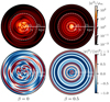 |
Fig. 7. Top row: Wave function density |ψ|2, i.e., the static terms shown in Fig. 6 and the interference term, as a function of the anisotropy parameter. Bottom row: Interference modulates the density comparable to the magnitude of the background density leading to a concentric ring pattern for the radially biased case (right column) and a more mixed interference fringe configuration under isotropic conditions (left column). |
In Fig. 8 we depict a selection of filament cross sections for an isotropic background density and a range of FDM masses 1 × 10⁻²² eV ≤ m ≤ 8 × 10⁻²² eV at z = 4.
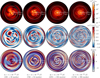 |
Fig. 8. Reconstructed FDM interference as a function of axion mass for an isotropic background density at redshift z = 4. First row: FDM density, |ψ|2, as in Eq. (5), i.e., including both the time static and interference term. Second row: The interference term relative to static background density. Strong, 𝒪(1), interference features are observable both in the radial and azimuthal direction, indicative of an isotropic, β = 0, background density. Third row: The wave function phase Arg[ψ]. Quantized vortices (red circles, shown only for the left hand column), another feature unique for FDM, correspond to 2π discontinuities in the phase function, or as described in the main text, places of nonzero vorticity, Eq. (30). |
Evidently, as the particle mass increases the fringe spacing in both the radial and azimuthal direction decreases, cf. first row. In all cases, however, the overall density is strongly modulated and incurs 𝒪(1) changes with respect to the background, cf. second row.
Since the wave function ψ is the superposition of single-valued eigenstates, ψ is single-valued too. Consequently, the circulation Γ related to the phase difference that arises from transporting the phase Θ = Arg[ψ] around any closed loop γ must be quantized:
 (29)
(29)
If γ encloses no roots of the wave function, the winding number n vanishes and the dynamics within this region may be expressed in terms of a potential flow v ∝ ∇Θ obeying the Madelung equations.
In the presence of destructive interference, however, roots can occur and if γ contains such loci – so-called quantum vortices – then n > 0. Put differently, vortices act as discrete sources of vorticity ∇ × v and interference can generate them. Since the Madelung formulation makes ∇ × v = 0 manifest, quantum vortices can only arise if we solve Eq. (1a) or Eq. (3a) which pose no restrictions on the value of the circulation except for Eq. (29). It is thus no surprise that the wave functions of Fig. 8 host interference-induced quantum vortices, which we locate for m = 1 × 10⁻²² eV as peaks in the vorticity,
 (30)
(30)
cf. red circles in the third row. As expected, these loci coincide with regions where the phase Θ wraps around once, that is, n = 1.
An extensive account on theoretical and observational consequences of quantum vortices for wave DM halos is given in Hui et al. (2021). For filaments, Alexander et al. (2022) conjectured that a sufficiently large number of vortex lines may generate a bulk rotation that is consistent with recent observations (Wang et al. 2021). Reconstructing this vortex population according to the prescription of the present work may be a way to test this hypothesis systematically7.
3. Statistical aspects of FDM filaments
With an idealized model for FDM filaments at hand, we turn our focus to a statistical characterization of fuzzy cosmic filaments. Section 3.1 investigates general population statistics and derives the mass function for FDM filaments. This will allow us to promote our effectively two-dimensional, single cylinder considerations of Sect. 2.4 to a three dimensional filament population. Mathematical details for the construction of the filament mass function are deferred to Appendix C. Section 3.2 analyzes how the matter power spectrum is modified in the presence of interference. Appendix D summarizes its computation – more precisely the one-filament contribution.
3.1. The filament mass function
The formation of the cosmic web constituents can be understood as a direct consequence of the ellipsoidal collapse model, (e.g., White & Silk 1979; Peebles 1980; Bond & Myers 1996). Tidal forces shear spherical patches centered around the peaks of the high-redshift Gaussian density field into a triaxial geometry. These initial, ellipsoidal overdensities continue to evolve under their self-gravity, external tides and Hubble expansion. Appendix C summarizes relevant contributions in detail (Bond & Myers 1996).
We illustrate an example evolution in the principal axis system of the ellipsoid for a ΛCDM background with concordance parameters (Planck Collaboration VI 2020) in Fig. 9. Depicted are the principal axes’ scale factors ai which relate to the physical axis size via the initial radius of the undeformed, spherical Lagrangian space patch by r(a) = ai(a)Rini. The initial conditions were constructed for a filament of mass M = 5 × 10⁹ h−1 M⊙ and tuned to allow for filament formation at z = 4 (Sheth et al. 2001) in the sense that we describe shortly. One may regard Fig. 9 as the idealized evolution of the smooth background density that leads to the fuzzy filament shown in Fig. 1.
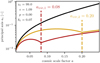 |
Fig. 9. Example of ellipsoidal collapse in a ΛCDM background for a homogeneous ellipsoid with mass M = 5 × 10⁹ M⊙ h−1. The equation of motion, Eq. (C.1), preserves the homogeneity of the initial conditions and it is thus sufficient to observe the evolution of the axis scale factors ai(a). After an initial expansion, each axis turns around, contracts and freezes out according to the steady-state tensor virial theorem, Eq. (C.6). The subsequent evolution is fixed to ensure a constant comoving axis size Ri = ai(a)Rini/a. We identify a filament as an object with two frozen axes – in the depicted scenario realized at z = 4. The residual triaxiality, i.e., the mismatch between the yellow and red lines at large a, is ignored for the construction of our filament population. |
The evolution proceeds in a self-similar, homogeneity-preserving fashion – a consequence of the quadratic nature of the ellipsoid’s potential. Each axis undergoes a Hubble flow driven expansion phase, followed by a turn around, gravity-induced contraction and subsequent freeze-out.
Note that both the transition redshift from contraction to freeze-out and its subsequent evolution are not a direct consequence of the equations of motion Eq. (C.1), but must be imposed by hand. A variety of approaches exist depending on the sought-after properties of the post-freeze out state: Bond & Myers (1996), Sheth et al. (2001) halt and freeze the collapse of principal axis i at ai(a)/a = f = 0.177. This ensures that, after the last axis collapsed, the nonlinear density contrast is consistent with a virialized halo under spherical collapse. In an Einstein-de Sitter (EdS) background, this implies:
 (31)
(31)
Desjacques (2008) analyzes the dependence between ellipsoidal protohalos and their environment and adopts the same freeze-out condition as Bond & Myers (1996), but makes angular momentum conservation subsequently manifest. Angrick & Bartelmann (2010) note that the value of f = 0.177 has no fundamental motivation for nonspherical collapse and therefore apply the steady-state tensor viral theorem to the evolving ellipsoidal density to derive a theoretically well-motivated per axis freeze-out radius, cf. Eq. (C.6).
In what follows, we adopt the approach that is most consistent with our steady-state cylinder considerations of Sect. 2.2. We freeze each axis once the tensor virial theorem is compatible with a steady-state configuration (Angrick & Bartelmann 2010), cf. Eq. (C.6), and enforce a constant comoving radius afterwards. A filament is then identified as an object for which two out of the three principal axes are frozen (Shen et al. 2006; Fard et al. 2019) and we see that enforcing a constant comoving axis-length reduces the triaxiality at filament formation so that a cylindrical approximation becomes viable.
How many of such defined filaments do we expect per comoving volume at formation redshift z? The excursion set formalism (Bond et al. 1991) provides an answer to this given two additional ingredients. The filament mass variance σ2(M), Eq. (C.7), and δec(σ2, z), that is, the linearly extrapolated density contrast at the time of filament formation according to ellipsoidal collapse evolution. Here we only give a brief account of the choices made to compute both quantities. We refer to Appendix C for mathematical details.
The mass variance σ2(M) results from smoothing the cosmic density field via a window function of spatial scale R (or equivalently mass scale M), cf. Eq. (C.7). The suppression properties of FDM are encoded in σ2(M) by virtue of its linear power spectrum entering the smoothing operation. The translation from spatial scale R to filament mass M depends on the choice of window function, which must be sufficiently sharp in k-space to ensure that the mass function remains sensitive to suppressive features encoded in the matter power spectrum (Schneider et al. 2013). In accordance with Du et al. (2024), we adopt a calibrated smooth-k filter (Leo et al. 2018; Bohr et al. 2021) for this task. In the end, we restrict our analysis to filament masses unaffected by the choice of filter.
For the linear density contrast at filament formation δec(σ2, z), one commonly employs fitting formulae derived from ellipsoidal collapse studies. Shen et al. (2006) provide such a fit in the case of an EdS background and ad hoc freeze-out condition Eq. (31). Since we are not aware of a similar result for the virial freeze-out condition Eq. (C.6) in ΛCDM, we determine δec(σ2, z) by optimizing the initial ellipsoidal over density δ(aini ∣ M), until we are able to form filaments of mass M at redshift z. Linear theory is then used to extrapolate forward again, that is:
 (32)
(32)
with D(z) as the ΛCDM growth factor (Dodelson 2003). Scale-dependent FDM growth is irrelevant on the filament scales that we consider here.
The number of filaments with masses between M and M + dM at redshift z, that is, the filament mass function (FMF), then follows from:
 (33)
(33)
with ρm0 and fB as present-day matter density and multiplicity function of the barrier,
 (34)
(34)
respectively. Details on the computation of the multiplicity function are deferred to Appendix C.
Figure 10 depicts the FMF for a selection of FDM masses at redshift z = 4. The low-mass suppression is the result of the small-scale suppression of matter power due to the presence of quantum pressure – a property of the diffusive, kinetic term in Eq. (1a). We also show the FMF obtained if the freeze-out condition Eq. (31) (dashed) is used instead of Eq. (C.6) (solid). The dashed FMF can be understood as the ΛCDM variant of the FMF derived in Shen et al. (2006). We find no deviations for M < 1011 h−1 M⊙.
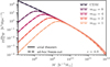 |
Fig. 10. Filament mass function (FMF) for various FDM masses at redshift z = 4. The suppression in the linear FDM power spectrum translates to a power suppression for filament masses. For filament masses M > 3 × 10⁹ h−1 M⊙, all considered FDM cases are indistinguishable from CDM and it is in this regime in which we sample the FMF in order to guarantee the same overall number density and thus same significance of interference effects measured in the correlation functions discussed in Sect. 3. |
The FMF together with the geometry of the final ellipsoidal state may also be used to promote our effectively two-dimensional, single filament considerations of Sect. 2 to a simplified, three-dimensional filament population, To this end, we translate the total filament mass into initial conditions for the ellipsoidal collapse (Sheth et al. 2001), follow the principal axis evolution until z = 4 and map the strongly prolate, final ellipsoid to a cylindrical geometry. More precisely, we set:
 (35)
(35)
 (36)
(36)
as the comoving length and radius containing 90% of the total line mass μ. Equation (11) then provides the per-cylinder velocity dispersion σ2 if we identify μ ≡ M/L. With these parameters at hand, we construct the eigenstate library, compute the phase space distribution and optimize the wave function coefficients to arrive at a semi-analytical expression for ψ.
Next, we assume a fiducial, longitudinal profile of the form:
![Mathematical equation: $$ \begin{aligned} \lambda (Z\mid L) = \frac{1}{2}\left[ \mathrm{erf} \left(\Delta \left(z + \frac{L}{2}\right)\right) - \mathrm{erf} \left(\Delta \left(z - \frac{L}{2}\right)\right) \right] ,\; \Delta = \frac{10}{L}, \end{aligned} $$](/articles/aa/full_html/2025/04/aa54232-25/aa54232-25-eq47.gif) (37)
(37)
such that
 (38)
(38)
constitute the CDM/FDM filament densities, smoothly restricted to Z = ±L/2 along the filament spine.
Figure 11 illustrates an example realization of our filament population assuming cylinder locations {xi}i = 1…N and orientations {di}i = 1…N follow from:
![Mathematical equation: $$ \begin{aligned} \boldsymbol{x}_i \sim U([0, L]^3),\; \boldsymbol{d}_i \sim S^2 . \end{aligned} $$](/articles/aa/full_html/2025/04/aa54232-25/aa54232-25-eq49.gif) (39)
(39)
Samples are accepted if no cylinders overlap in the fundamental cell and all its periodic extensions, which would violate our assumption of all filaments being gravitationally isolated. This clearly ignores any large scale filament-filament cross-correlation imprinted on the cosmic web (which, in analogy to the halo model, at leading order should be given by the linear power spectrum). More refined placement techniques, in particular a peak-patch description (Bond & Myers 1996) may be used to alleviate this shortcoming.
3.2. The matter power spectrum
How are two-point density correlations impacted by the presence of interference in filaments? To answer this, we turn to the isotropic power spectrum:
 (40)
(40)
Fully-fledged cosmological simulations of FDM report an excess correlation in the FDM matter power spectrum compared to its CDM counterpart for highly nonlinear k > 𝒪(100) h Mpc−1 (Veltmaat & Niemeyer 2016; Mocz et al. 2020; May & Springel 2021, 2023; Laguë et al. 2024), and conjectured, quite intuitively, this power boost to originate from interference fringes imprinted on the density field |ψ|2. The wave function reconstruction scheme of Sect. 2 combined with the population statistics developed in Sect. 3.1 allow us to test if quasi-virial filaments can in principle be the source of such a power boost.
Interference is a local phenomenon, that is, the result of trapped wave modes beating against each other in a common gravitational potential sourced by a single filament. One should not expect any correlation from the interference dynamics between sufficiently separated filaments. Section 2 makes this manifest by treating the wave function reconstruction ex situ.
Motivated by the standard halo model (Cooray & Sheth 2002), we therefore decompose Eq. (40) into a one-filament, P1f(k), and two-filament contribution, P2f(k). The two-filament term captures correlation between filaments. We ignore this in the present model, since the cross-correlation of filaments will not contain an interference term, and as already noted at leading order is captured by the linear power spectrum.
The one filament term reads:
 (41)
(41)
and measures the spatial correlation at the ensemble level by stacking isotropized spectra of individual filaments:
 (42)
(42)
 (43)
(43)
of total mass M.
For the density depicted in Fig. 11, we expect P(k) = P1f(k) since filament-filament cross-correlations are suppressed by construction. This is supported by computing P(k) for the box shown in Fig. 11 (dashed) and comparing it against P1f(k) from Eq. (41) (solid) in the bottom panel of Fig. 12. Thus, populating a three dimensional box as described in Sect. 3.1 and subsequent k-space binning is a simple way to compute the one-filament term. However, the obvious tension between a large domain (better statistics due to more filaments) and sufficient resolution to resolve the finest interference fringes gets quickly intractable as the FDM mass increases.
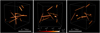 |
Fig. 11. Volume rendering of the idealized FDM filament sample for m22 = 1 in a periodic, comoving box of L = 2 h−1 Mpc at z = 4, generated by sampling the FMF in Fig. 10 for masses M > 3 × 10⁹ h−1 M⊙. The same realization is shown from three different viewing angles. The characteristic filament length is ≃1 − 2 h−1 Mpc. The random iid placement of the cylinders neglects any filament-filament cross-correlations encoded in the cosmic web. Consequently, one expects the power spectrum of the box shown to be identical to the one-filament term in Eq. (41). This is supported by Fig. 12 which compares the spectrum of the domain depicted in this Figure (dashed, yellow) with the stacked spectra following from Eq. (41) (solid, blue). |
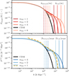 |
Fig. 12. Three-dimensional filament matter power spectra of the interference-free CDM background and the reconstructed FDM density for a selection of FDM masses at z = 4. Top: Single filament spectrum, Psingle(k ∣ M), for an example filament of total mass M = 5 × 10⁹ h−1 M⊙. One finds all FDM spectra to be compatible with CDM down to the spatial extent of the ground state, Rgs ≡ ⟨ψ0|R|ψ0⟩ (vertical, dashed line) – effectively the characteristic scale of the cylinder. Once sufficiently small scales inside the filament are probed, the interference contribution to |ψ|2 enhances the two point density correlation and boosts Psingle(k ∣ M) above the CDM baseline. Note that for larger m22: (i) Psingle(k ∣ M) detaches later from the CDM baseline, (ii) the boost is shallower but (iii) extends to higher k until the suppression scale kcut ∝ m is reached (vertical, solid lines). Bottom: One-filament term P1f(k) – a stacked version of many Psingle(k ∣ M), weighted according to the FMF in Fig. 10. We limit the filament population to the mass window M ∈ [3×10⁹, 3×10¹⁰] h−1 M⊙ and compute the one filament term either directly from the semi-analytical expression of the wave function developed in Appendix D (solid, blue) or by populating a box as shown in Fig. 11 (dashed, yellow). All quantitative observations made for the single cylinder case translate to P1f(k) after a FMF-weighted average according to Eq. (45), i.e., Rgs → ⟨Rgs⟩FMF (vertical, dashed lines) and kcut → ⟨kcut⟩FMF (vertical, solid lines). |
Fortunately, we have access to ψ and have explicitly reduced its library size. Therefore, it is advantageous to compute P1f according to Eq. (41), that is, by directly stacking a large number of single-filament spectra, Psingle(k|M). This approach also allows us to consider the effects of interference at the level of individual filaments before generalizing to P1f(k). Technical details are provided in Appendix D.
The top panel of Fig. 12 depicts the single filament power spectrum Psingle(k∣M = 5×10⁹ h−1 M⊙), for a selection of FDM masses (shades of red) alongside the interference free CDM case (black).
Comparing the FDM spectra with the CDM spectrum, we find a boost in matter power for k > 100 h kpc−1, which we can attribute exclusively to the presence of the interference cross-terms in |ψ|2.
In all considered cases, the FDM spectrum detaches from the CDM baseline at some wavenumber kdetach, once the reciprocal correlation wavenumber k starts to probe scales interior to the filament. The exact value of kdetach is observed to have a weak, monotonically increasing, dependence in m22 and we find it to be reasonably well approximated by the expectation value of the radial position operator with respect to the ground state mode, that is, kdetach ∝ ⟨ψ0|R|ψ0⟩−1 (dashed, vertical lines). This, together with the shallower boost for higher FDM mass, is consistent with our expectation of recovering the CDM scenario in the limit m22 → ∞.
The power boost extends to higher k until a FDM mass-dependent cut-off scale kcut(m) drives Psingle(k) to zero. We interpret this scale as a nonlinear extension of the linear Jeans suppression scale set by the uncertainty principle ucutxcut ≳ m−1ℏ. Figure 12 suggests kcut(m)∝m such that the conjugate velocity ucut entering the uncertainty relation must be mass independent. As most interference is located in the filament outskirts where high energy and angular momenta modes dominate, it is intuitive to associate ucut with the FDM mass independent, WKB behavior of the mode coefficients |anl|2 ∝ f(E). We therefore return to the isotropic phase space distribution shown in Fig. 4 (black, dashed line), which for E/V(R99) > 0.1 is well described by an isothermal distribution (Binney & Tremaine 2008) of the form:
 (44)
(44)
Fitting the isothermal ansatz to Fig. 4 and setting  results in the solid, vertical lines shown in Fig. 12 which are in satisfying agreement with the suppression cut-off of the interference boost.
Figure 12’s bottom panel depicts the one-filament term P1f(k) for m22 = 1, 2, 4 restricted to an ensemble with mass M ∈ [3×109,3×1010] h−1 M⊙. The lower total mass limit is chosen such that CDM and all considered FDM cases have identical population statistics according to the suppression physics encoded in the linear power spectrum, cf. Fig. 10. The upper limit is set by resource constraints8.
Let ⟨Q⟩FMF denote the FMF-weighted average of quantity Q:
 (45)
(45)
We then recover the same qualitative behavior as seen in Psingle(k) upon applying an FMF-average, that is, one finds large scale equivalence with CDM, departure once scales smaller than ⟨⟨ψ0|R|ψ0⟩⟩FMF are reached, and a sustained boost in power up to ⟨kcut(m)⟩FMF.
4. Discussion
Let us put these results into context. As stated in our introductory remarks, interference, not just in filaments but in all constituents of the cosmic web, has been identified as a smoking gun signature since the advent of FDM simulations (Schive et al. 2014). State-of-the-art SP numerics allows us to follow FDM structure formation from the kpc scale up to boxes of size L = 10 h−1 Mpc and down to z ≳ 0. This is sufficient to resolve the impact of wave phenomena on summary statistics for a canonical FDM mass of m22 < 1 (May & Springel 2021, 2023). For the matter power spectrum, the wave-like signatures may be summarized as follows.
For sufficiently high redshift, z ≥ 5, the difference between CDM and FDM dynamics is negligible compared to the influence of the initial conditions (May & Springel 2021, 2023) – the classical FDM approximation is thus justified in this regime. At lower redshift, however, the impact of FDM’s wave-like evolution is more significant and introduces two additional features in P(k) compared to its CDM counterpart and irrespective of the choice of initial conditions: (i) larger scales, k ≲ 𝒪(10) h Mpc−1, are suppressed and (ii) smaller scales, k ≳ 𝒪(100) h Mpc−1, experience an enhancement.
Our proof-of-concept analysis indicates that interference induced by a steady-state fuzzy filament population can produce the observed power boost on scales broadly consistent with Mocz et al. (2019), May & Springel (2021, 2023). The impact of wave dynamics on larger, quasi-linear scales is not accessible by our model. Intuitively, one would expect their evolution to be better described perturbatively, that is, by means of a wave equivalent of Zeldovich’s approximation, that captures the coherent flow of matter waves, rather than the quasi-virial limit our filament proxies assume.
Uhlemann et al. (2019) provide such a description via the propagator perturbation technique (PPT). From the perspective of interference/wave modeling, the crucial difference between PPT and classical Lagrangian methods (LPT) is the representation of the cosmic density as a semiclassical wave function rather than a set of fluid test particles9. Thus, wave effects are retained in PPT up to mildly nonlinear scales.
Gough & Uhlemann (2024) deployed PPT to analyze the impact of wave effects, that is, interference and quantum pressure, on summary statistics for spatial scales accessible to a perturbative treatment. In case of the matter power spectrum at z = 4, wave-like PPT evolution produced a suppression of power for scales k ≲ 10 h Mpc−1 compared to the CDM LPT dynamics. This result was found to be in broad agreement with the m22 = 0.1 SP simulations of May & Springel (2023).
Together, PPT and the interference reconstruction of this work thus provide a complementary picture that is in qualitative accordance with simulation results and suggests the following intuitive picture. Up to mildly-nonlinear scales, FDM flows coherently into the gravitational wells of over dense regions and quantum pressure suppresses structure, even if interference is taken into account. Nonlinear scales, by contrast, are boosted by the interference emerging in objects such as filaments until Heisenberg’s uncertainty suppresses structure growth entirely.
At present, observed quasar absorption spectra allow us to probe P(k) down to k ≃ 𝒪(10) h Mpc−1 (Boera et al. 2019), while interference from our filament population enhances scales at least two orders of magnitude smaller and way past the filtering scale kf ≃ 40 h Mpc−1 (Hui & Gnedin 1997). We conclude that steady-state filaments, as described in this work, are not expected to affect ultralight DM constraints from the Lyα forest (e.g., Iršič et al. 2017; Kobayashi et al. 2017; Rogers & Peiris 2021) due to a degeneracy between linear quantum pressure suppression and interference enhancement. This further justifies the use of the “classical FDM” approximation, that is, FDM initial conditions for CDM simulations, for modeling mildly nonlinear scales probed by the Lyα forest.
Interestingly, the mass dependence of kdetach and kcut indicates that axions lighter than those considered in this work may be sensitive to this degeneracy at larger spatial scales. At the same time, a lower value of m22 implies fewer eigenstates and consequently reduced interference enhancement at fixed k relative to the CDM baseline. Focusing on higher-mass filaments at redshifts z < 4 may help maintain the amplitude of the interference bump, while shifting to scales accessible to large-scale structure probes.
A natural question is to what extent interference in virialized, spherically symmetric halos contributes to small scale modifications in P(k). Answering this in detail is beyond the scope of this work. Here, we only state that at high redshift, z > 3, halos were found to contribute more than an order of magnitude less bound mass to the cosmic web than filaments (Dome et al. 2023b). This should translate to a suppressed halo mass function relative to the FMF and consequently a reduced significance of P1h compared to P1f, cf. Eq. (41). At the level of individual filaments, the matching symmetry between the isotropized power spectrum and the spherically symmetric wave function results in cross-term cancellation for certain angular momentum combinations10. Moreover, halos are more compact and occupy less volume than filaments (Dome et al. 2023b). We therefore expect a higher value of kdetach. Higher characteristic velocities inside halos translate to higher values of kcut. In conclusion, we anticipate a power boost due to halo interference to be present at smaller scales and significantly reduced amplitude compared to filaments.
5. Conclusion and prospects
In this work, we took initial steps toward a more principled understanding of the modeling and measurability of interference features in FDM filaments. To this end:
-
We approximated FDM filaments as infinitely long, cylindrical objects, computed their associated eigenstates and superposed these states such that a (non)-isotropic, isothermal, steady-state solution of the classical Jeans equation is recovered. To reduce the complexity of the reconstructed wave function, we computed a self-consistent phase space model for cold filaments and leveraged the WKB correspondence between mode coefficients and phase-space distribution to perform a data-driven mode selection. We find the interference sourced by our simplified filament model to be in qualitative accordance with filament interference found in full SP simulations.
-
We applied the ellipsoidal collapse model alongside a virial freeze-out condition to construct a fuzzy filament mass function. Combined with the geometry of the partially collapsed ellipsoid, this approach allowed us to build a toy filament population that neglects filament-filament cross-correlations, but incorporates interference fringes generated by eigenstate cross-terms.
-
Using this toy population, we computed the one-filament matter power spectrum for various FDM masses. Our proof-of-concept analysis revealed a boost in power between the spatial scale associated with the ground state mode and the scale set by Heisenberg’s uncertainty principle at the root mean square velocity of the classical phase-space distribution. These findings are consistent with fully-fledged SP simulations (Mocz et al. 2019; May & Springel 2021, 2023) and complement interference-sensitive, perturbative treatments of FDM structure formation (Gough & Uhlemann 2024).
Our work opens several avenues for extension. Below, we outline an incomplete list of directions:
-
Borne out of theoretical simplicity (Stodólkiewicz 1963; Ostriker 1964; Eisenstein et al. 1997) and numerical evidence (Ramsøy et al. 2021), we focused on an isothermal, steady-state approximation for filaments. However, a deeper understanding of the dynamical state of FDM filaments remains elusive. An ideal test bed to make progress on this question is the fuzzy filament catalog of May & Springel (2023). Assessing to which degree steady-state conditions are attained on a per filament basis may give insights into the relative abundance of this subpopulation and is thus a natural next step. Moreover, stacking the catalog would provide access to the one-filament spectrum which could be directly compared with our bottom-up model.
-
An intriguing prospect is to merge PPT and interference reconstruction. This may be achieved by combining PPT with the aforementioned peak-patch algorithm (Bond & Myers 1996) to propagate FDM initial conditions to a target redshift, smooth the resulting density field on mass scale M and identify peaks above the critical density suggested by ellipsoidal collapse. Upon replacing these patches with the fuzzy cylinders developed in this work, one arrives at a density field with consistent large scale suppression, small scale enhancement of structure and correct filament-filament cross-correlation.
-
We have alluded to the possibility of using the presented model as a N-body simulation post-processing tool, in which particle positions and velocities inside filaments may be used to reconstruct the wave function (see the discussion around Eq. (27)) and phase space distribution (Schwarzschild 1979).
-
Beyond the semi-analytical treatment in this work, a Gaussian beam decomposition of ψ and subsequent integration of the beam trajectories (Schwabe & Niemeyer 2022) is appealing for nonstationary conditions. In this approach, phase information is retained and carried along the traveling beams such that interference can be reconstructed locally by summing over all beams.
-
Having identified P1f – the stacked single filament power spectrum – as a statistic sensitive to interference fringes, we speculate that the weak lensing signal of stacked filaments may be used to reconstruct the surface mass density (e.g., Lokken et al. 2024) and thus the one-filament power spectrum observationally. This may pave the way for a novel ultralight DM mass limit based on interference alone11.
-
Gough & Uhlemann (2024) advocate to study the implications of interference on statistics beyond two-point functions. A particularly interesting observable is the line correlation function (LCF) (Obreschkow et al. 2013; Wolstenhulme et al. 2015; Eggemeier et al. 2015). The LCF is a regularized version of the three-point correlator
 , designed to capture information contained in the phases,
  , of the density field. Not only does the LCF quantify statistical information absent in the power spectrum, it also measures the degree of straight filamentarity on the spatial scale R (Obreschkow et al. 2013). Therefore, we anticipate the LCF to be an intriguing summary statistic able to quantify interference in filaments. We have already done some preliminary work on this subject and refer to the github repositories below for an unoptimized Python implementation.
Data availability
GitHub: The code used to generate the results in this work can be found at  timzimm/fuzzylli and
  timzimm/fdm_filaments.
This is a generalization of the isotropic, β = 0, case considered in Stodólkiewicz (1963), Ostriker (1964).
Embedding the cylinder into the isothermal solution of a steady-state sheet improves the correspondence with the simulated density profiles even further. Since our focus is on filaments only, we neglect this contribution.
Adding an attractive, local interaction of the form λ|ψ|2ψ introduces a critical line mass μc above which even infinitely long cylinders are unstable and collapse radially.
To solve Eq. (17) in practice, we approximate log g(E) as a multilayer perceptron (Hastie et al. 2009), perform the numerical integration as forward pass and find the perceptron weights by minimizing the least square difference to ρBG.
Recall that we only fit up to R99.
For a numerical analysis of vortices in halos, see Liu et al. (2023).
Recall that Psingle now needs to be computed for a range of total masses M. Higher-mass filaments translate to deeper potential wells, imply more extensive eigenstate libraries and thus require us to solve more challenging optimization problems. Although parallelization strategies exist, we have not put significant effort into making the latter scalable.
In fact, to leading order, PPT is equivalent to free wave propagation.
More precisely, we find ⟨|u(k ∣ M)|2⟩|k|=k for a halo to depend on the Wigner-3j symbols for which selection rules apply.
It is interesting to note in this context that strong lensing can probe the existence of an interference substructure in radio arcs, providing an effective way to derive mass limits (Powell et al. 2023).
The astute reader may wonder, why we do not transform eq. (A.1) according to the discussion in Appendix B in order to recover a classical barrier shape ∝l2/R2 as this seems to recover a small radius power law asymptote with integer exponent. Unfortunately, if l = 0 inhomogeneous Dirichlet conditions are imposed at the domain boundaries for a Langer corrected version of eq. (A.1). This generalises the discrete problem to an inhomogeneous eigenvalue problem that is not straight forward to solve.
For fully isotropic halos (Yavetz et al. 2022), integrating out the angular momentum dependence renders the differences between eq. (B.5a) and the Langer-corrected wave function irrelevant.
Acknowledgments
We thank Alexander Eggemeier for useful discussions on the (anisotropic) line correlation function, Charis Pooni for valuable comments on the wave function reconstruction, as well as Simon May, Tibor Dome, Jens Niemeyer, Renée Hložek and Philip Mocz for enlightening comments on interference in FDM filaments. TZ would like to thank the Theoretical Particle Physics & Cosmology (TPPC) Group at King’s College London for their hospitality during the research stay, during which parts of this work were carried out. TZ acknowledges financial support through a Kristine Bonnevie stipend (University of Oslo). DJEM is supported by an Ernest Rutherford Fellowship from the Science and Technologies Facilities Council (ST/T004037/1). KKR is supported by an Ernest Rutherford Fellowship from the Science and Technologies Facilities Council (ST/Z510191/1). The Dunlap Institute is funded through an endowment established by the David Dunlap family and the University of Toronto. This project has received funding from the European Union’s Horizon 2020 research and innovation programme under the Marie Skłodowska-Curie grant agreement No. 945371.
References
- Alexander, S., Capanelli, C., Ferreira, G. M. E., & McDonough, E., 2022, Phys. Lett. B, 833, 137298 [Google Scholar]
- Angrick, C., & Bartelmann, M. 2010, A&A, 518, A38 [NASA ADS] [CrossRef] [EDP Sciences] [Google Scholar]
- Aragón-Calvo, M. A., Weygaert, R. V. D., & Jones, B. J. T. 2010, MNRAS, 408, 2163 [CrossRef] [Google Scholar]
- Armengaud, E., Palanque-Delabrouille, N., Yèche, C., Marsh, D. J. E., & Baur, J. 2017, MNRAS, 471, 4606 [NASA ADS] [CrossRef] [Google Scholar]
- Arvanitaki, A., Dimopoulos, S., Dubovsky, S., Kaloper, N., & March-Russell, J. 2010, Phys. Rev. D, 81, 123530 [NASA ADS] [CrossRef] [Google Scholar]
- Baddour, N. 2009, J. Opt. Soc. Am. A, 26, 1767 [NASA ADS] [CrossRef] [Google Scholar]
- Banik, N., Bovy, J., Bertone, G., Erkal, D., & de Boer, T. J. L. 2021, JCAP, 10, 043 [CrossRef] [Google Scholar]
- Bartelmann, M. 2015, Phys. Rev. D, 91, 083524 [Google Scholar]
- Benson, A. J., Farahi, A., Cole, S., et al. 2013, MNRAS, 428, 1774 [NASA ADS] [CrossRef] [Google Scholar]
- Berry, M. V., & Mount, K. E. 1972, Rep. Prog. Phys., 35, 315 [Google Scholar]
- Berry, M. V., Almeida, A. M. O. D., 1973, J. Phys. A: Math. Nucl. Gen., 6, 1451 [NASA ADS] [CrossRef] [Google Scholar]
- Binney, J., & Tremaine, S. 2008, Galactic Dynamics (Princeton University Press) [Google Scholar]
- Boera, E., Becker, G. D., Bolton, J. S., & Nasir, F. 2019, ApJ, 872, 101 [NASA ADS] [CrossRef] [Google Scholar]
- Bohr, S., Zavala, J., Cyr-Racine, F.-Y., & Vogelsberger, M. 2021, MNRAS, 506, 128 [CrossRef] [Google Scholar]
- Bond, J. R., & Myers, S. T. 1996, ApJS, 103, 1 [NASA ADS] [CrossRef] [Google Scholar]
- Bond, J. R., Cole, S., Efstathiou, G., & Kaiser, N. 1991, ApJ, 379, 440 [NASA ADS] [CrossRef] [Google Scholar]
- Cicoli, M., Guidetti, V., Righi, N., & Westphal, A. 2022, J. High Energy Phys., 2022, 107 [CrossRef] [Google Scholar]
- Colberg, J. M., Krughoff, K. S., & Connolly, A. J. 2005, MNRAS, 359, 272 [NASA ADS] [CrossRef] [Google Scholar]
- Cooray, A., & Sheth, R. 2002, Phys. Rep., 372, 1 [Google Scholar]
- Dalal, N., & Kravtsov, A. 2022, Phys. Rev. D, 106, 063517 [NASA ADS] [CrossRef] [Google Scholar]
- Dalal, N., Bovy, J., Hui, L., & Li, X. 2021, JCAP, 2021, 076 [CrossRef] [Google Scholar]
- Dejonghe, H. 1986, Phys. Rep., 133, 217 [NASA ADS] [CrossRef] [Google Scholar]
- Dentler, M., Marsh, D. J. E., Hložek, R., et al. 2022, MNRAS, 515, 5646 [NASA ADS] [CrossRef] [Google Scholar]
- Desjacques, V. 2008, MNRAS, 388, 638 [NASA ADS] [CrossRef] [Google Scholar]
- Desjacques, V., Kehagias, A., & Riotto, A. 2018, Phys. Rev. D, 97, 023529 [Google Scholar]
- Dodelson, S. 2003, Modern Cosmology (Oxford: Elsevier LTD) [Google Scholar]
- Dolag, K., Meneghetti, M., Moscardini, L., Rasia, E., & Bonaldi, A. 2006, MNRAS, 370, 656 [NASA ADS] [Google Scholar]
- Dome, T., Fialkov, A., Mocz, P., et al. 2023a, MNRAS, 519, 4183 [NASA ADS] [CrossRef] [Google Scholar]
- Dome, T., Fialkov, A., Sartorio, N., & Mocz, P. 2023b, MNRAS, 525, 348 [NASA ADS] [CrossRef] [Google Scholar]
- Du, X., Behrens, C., & Niemeyer, J. C. 2016, MNRAS, 465, 941 [Google Scholar]
- Du, X., Marsh, D. J. E., Escudero, M., et al. 2024, Phys. Rev. D, 109, 043019 [Google Scholar]
- Eggemeier, A., Battefeld, T., Smith, R. E., & Niemeyer, J. 2015, MNRAS, 453, 797 [NASA ADS] [CrossRef] [Google Scholar]
- Eisenstein, D. J., Loeb, A., & Turner, E. L. 1997, ApJ, 475, 421 [NASA ADS] [CrossRef] [Google Scholar]
- Fard, M. A., Taamoli, S., & Baghram, S. 2019, MNRAS, 489, 900 [NASA ADS] [CrossRef] [Google Scholar]
- Fiege, J. D., & Pudritz, R. E. 2000, MNRAS, 311, 85 [Google Scholar]
- Garny, M., Konstandin, T., & Rubira, H. 2020, JCAP, 2020, 003 [NASA ADS] [CrossRef] [Google Scholar]
- Gough, A., & Uhlemann, C. 2024, Open J. Astrophys., 7, 60 [Google Scholar]
- Hamilton, A. J. S. 2000, MNRAS, 312, 257 [NASA ADS] [CrossRef] [Google Scholar]
- Harmany, Z. T., Marcia, R. F., & Willett, R. M. 2012, IEEE Trans. Image Process., 21, 1084 [CrossRef] [Google Scholar]
- Hastie, T., Tibshirani, R., & Friedman, J. 2009, The Elements of Statistical Learning (New York: Springer) [Google Scholar]
- Hejlesen, M. M., Winckelmans, G., & Walther, J. H. 2019, Appl. Math. Lett., 89, 28 [CrossRef] [Google Scholar]
- Hlozek, R., Grin, D., Marsh, D. J. E., & Ferreira, P. G. 2015, Phys. Rev. D, 91, 103512 [NASA ADS] [CrossRef] [Google Scholar]
- Hlozek, R., Marsh, D. J. E., & Grin, D. 2018, MNRAS, 476, 3063 [CrossRef] [Google Scholar]
- Hu, W., Barkana, R., & Gruzinov, A. 2000, Phys. Rev. Lett., 85, 1158 [NASA ADS] [CrossRef] [Google Scholar]
- Hui, L. 2021, ARA&A, 59, 247 [NASA ADS] [CrossRef] [Google Scholar]
- Hui, L., & Gnedin, N. Y. 1997, MNRAS, 292, 27 [Google Scholar]
- Hui, L., Ostriker, J. P., Tremaine, S., & Witten, E. 2017, Phys. Rev. D, 95, 043541 [NASA ADS] [CrossRef] [Google Scholar]
- Hui, L., Joyce, A., Landry, M. J., & Li, X. 2021, JCAP, 2021, 011 [CrossRef] [Google Scholar]
- Hunter, C., & Qian, E. 1993, MNRAS, 262, 401 [Google Scholar]
- HyeongHan, K., Jee, M. J., Cha, S., & Cho, H. 2024, Nat. Astron., 8, 377 [NASA ADS] [CrossRef] [Google Scholar]
- Iršič, V., Viel, M., Haehnelt, M. G., Bolton, J. S., & Becker, G. D. 2017, Phys. Rev. Lett., 119, 031302 [CrossRef] [Google Scholar]
- Iršič, V., Viel, M., Haehnelt, M. G., et al. 2024, Phys. Rev. D, 109, 043511 [Google Scholar]
- Khlopov, M., Malomed, B. A., & Zeldovich, I. B. 1985, MNRAS, 215, 575 [NASA ADS] [CrossRef] [Google Scholar]
- Kobayashi, T., Murgia, R., De Simone, A., Iršič, V., & Viel, M. 2017, Phys. Rev. D, 96, 123514 [NASA ADS] [CrossRef] [Google Scholar]
- Laguë, A., Bond, J. R., Hložek, R., et al. 2022, JCAP, 01, 049 [CrossRef] [Google Scholar]
- Laguë, A., Schwabe, B., Hložek, R., Marsh, D. J. E., & Rogers, K. K. 2024, Phys. Rev. D, 109, 043507 [Google Scholar]
- Laliena, V., & Campo, J. 2018, J. Phys. A Math. Gen., 51, 325203 [NASA ADS] [CrossRef] [Google Scholar]
- Langer, R. E. 1937, Phys. Rev., 51, 669 [Google Scholar]
- Ledoux, V., Ixaru, L., Rizea, M., Van Daele, M., & Berghe, G. V. 2006, Comput. Phys. Commun., 175, 612 [NASA ADS] [CrossRef] [Google Scholar]
- Leo, M., Baugh, C. M., Li, B., & Pascoli, S. 2018, JCAP, 2018, 010 [Google Scholar]
- Levkov, D. G., Panin, A. G., & Tkachev, I. I. 2018, Phys. Rev. Lett., 121, 151301 [Google Scholar]
- Lewis, H. R., & Bellan, P. M. 1990, J. Math. Phys., 31, 2592 [NASA ADS] [CrossRef] [Google Scholar]
- Lin, S.-C., Schive, H.-Y., Wong, S.-K., & Chiueh, T. 2018, Phys. Rev. D, 97, 103523 [Google Scholar]
- Liu, I. K., Proukakis, N. P., & Rigopoulos, G. 2023, MNRAS, 521, 3625 [NASA ADS] [CrossRef] [Google Scholar]
- Liu, Y., Gao, L., Liao, S., & Zhu, K. 2024, arXiv e-prints [arXiv:2409.11088] [Google Scholar]
- Lokken, M., van Engelen, A., Aguena, M., et al. 2024, ApJ, submitted [arXiv:2409.04535] [Google Scholar]
- Lukić, Z., Stark, C. W., Nugent, P., et al. 2015, MNRAS, 446, 3697 [CrossRef] [Google Scholar]
- Lynden-Bell, D. 1967, MNRAS, 136, 101 [Google Scholar]
- Marsh, D. J. E. 2016, Phys. Rep., 643, 1 [NASA ADS] [CrossRef] [Google Scholar]
- Marsh, D. J. E., & Hoof, S. 2023, eds. D. F. J. Kimball, & K. van Bibber The Search for Ultralight Bosonic Dark Matter, 73 [CrossRef] [Google Scholar]
- Marsh, D. J. E., & Niemeyer, J. C. 2019, Phys. Rev. Lett., 123, 051103 [CrossRef] [Google Scholar]
- Marsh, D. J. E., & Silk, J. 2014, MNRAS, 437, 2652 [NASA ADS] [CrossRef] [Google Scholar]
- May, S., & Springel, V. 2021, MNRAS, 506, 2603 [NASA ADS] [CrossRef] [Google Scholar]
- May, S., & Springel, V. 2023, MNRAS, 524, 4256 [NASA ADS] [CrossRef] [Google Scholar]
- Mead, J. M. G., King, L. J., & McCarthy, I. G. 2010, MNRAS, 401, 2257 [CrossRef] [Google Scholar]
- Mehta, V. M., Demirtas, M., Long, C., et al. 2021, JCAP, 07, 033 [CrossRef] [Google Scholar]
- Merritt, D. 1996, AJ, 112, 1085 [NASA ADS] [CrossRef] [Google Scholar]
- Mocz, P., & Succi, S. 2015, Phys. Rev. E, 91, 053304 [Google Scholar]
- Mocz, P., Lancaster, L., Fialkov, A., Becerra, F., & Chavanis, P.-H. 2018, Phys. Rev., D, 97 [Google Scholar]
- Mocz, P., Fialkov, A., Vogelsberger, M., et al. 2019, Phys. Rev. Lett., 123, 141301 [CrossRef] [Google Scholar]
- Mocz, P., Fialkov, A., Vogelsberger, M., et al. 2020, MNRAS, 494, 2027 [NASA ADS] [CrossRef] [Google Scholar]
- Nadler, E. O., Gluscevic, V., Boddy, K. K., & Wechsler, R. H. 2019, ApJ, 878, L32 [NASA ADS] [CrossRef] [Google Scholar]
- Navarro, J. F., Frenk, C. S., & White, S. D. M. 1996, ApJ, 462, 563 [Google Scholar]
- Nori, M., & Baldi, M. 2018, MNRAS, 478, 3935 [Google Scholar]
- Nori, M., & Baldi, M. 2021, MNRAS, 501, 1539 [Google Scholar]
- Nori, M., Murgia, R., Iršič, V., Baldi, M., & Viel, M. 2019, MNRAS, 482, 3227 [NASA ADS] [CrossRef] [Google Scholar]
- Obreschkow, D., Power, C., Bruderer, M., & Bonvin, C. 2013, ApJ, 762, 115 [NASA ADS] [CrossRef] [Google Scholar]
- Odekon, M. C., Jones, M. G., Graham, L., Kelley-Derzon, J., & Halstead, E. 2022, ApJ, 935, 130 [NASA ADS] [CrossRef] [Google Scholar]
- Ostriker, J. 1964, ApJ, 140, 1056 [Google Scholar]
- Parikh, N. 2014, Found. Trends Optim., 1, 127 [CrossRef] [Google Scholar]
- Peebles, P. J. E. 1980, Large-Scale Structure of the Universe (Princeton University Press) [Google Scholar]
- Petač, M., & Ullio, P. 2019, Phys. Rev. D, 99, 043003 [Google Scholar]
- Planck Collaboration VI. 2020, A&A, 641, A6 [NASA ADS] [CrossRef] [EDP Sciences] [Google Scholar]
- Powell, D. M., Vegetti, S., McKean, J. P., et al. 2023, MNRAS, 524, L84 [NASA ADS] [CrossRef] [Google Scholar]
- Ramsøy, M., Slyz, A., Devriendt, J., Laigle, C., & Dubois, Y. 2021, MNRAS, 502, 351 [Google Scholar]
- Rogers, K. K., & Peiris, H. V. 2021, Phys. Rev. D, 103, 043526 [NASA ADS] [CrossRef] [Google Scholar]
- Rogers, K. K., & Peiris, H. V. 2021, Phys. Rev. Lett., 126, 071302 [NASA ADS] [CrossRef] [Google Scholar]
- Rogers, K. K., & Poulin, V. 2025, Phys. Rev. Res., 7, L012018 [Google Scholar]
- Rogers, K. K., Peiris, H. V., Pontzen, A., et al. 2019, JCAP, 02, 031 [CrossRef] [Google Scholar]
- Rogers, K. K., Dvorkin, C., & Peiris, H. V. 2022, Phys. Rev. Lett., 128, 171301 [Google Scholar]
- Rogers, K. K., Hložek, R., Laguë, A., et al. 2023, JCAP, 06, 023 [CrossRef] [Google Scholar]
- Schive, H.-Y., Chiueh, T., & Broadhurst, T. 2014, Nat. Phys., 10, 496 [NASA ADS] [CrossRef] [Google Scholar]
- Schneider, A., Smith, R. E., & Reed, D. 2013, MNRAS, 433, 1573 [CrossRef] [Google Scholar]
- Schwabe, B., & Niemeyer, J. C. 2022, Phys. Rev. Lett., 128, 181301 [Google Scholar]
- Schwarzschild, M. 1979, ApJ, 232, 236 [NASA ADS] [CrossRef] [Google Scholar]
- Shen, J., Abel, T., Mo, H. J., & Sheth, R. K. 2006, ApJ, 645, 783 [NASA ADS] [CrossRef] [Google Scholar]
- Sheridan, E., Carta, F., Gendler, N., et al. 2024, arXiv e-prints [arXiv:2412.12012] [Google Scholar]
- Sheth, R. K., Mo, H. J., & Tormen, G. 2001, MNRAS, 323, 1 [NASA ADS] [CrossRef] [Google Scholar]
- Stodólkiewicz, J. S. 1963, Acta Astron., 13, 30 [NASA ADS] [Google Scholar]
- Talman, J. D. 1978, J. Comput. Phys., 29, 35 [NASA ADS] [CrossRef] [Google Scholar]
- Trefethen, L. N. 2000, Spectral Methods in MATLAB (Society for Industrial and Applied Mathematics) [CrossRef] [Google Scholar]
- Uhlemann, C., Kopp, M., & Haugg, T. 2014, Phys. Rev., D, 90 [Google Scholar]
- Uhlemann, C., Rampf, C., Gosenca, M., & Hahn, O. 2019, Phys. Rev. D, 99, 083524 [NASA ADS] [CrossRef] [Google Scholar]
- Veltmaat, J., & Niemeyer, J. C. 2016, Phys. Rev. D, 94, 123523 [Google Scholar]
- Viel, M., Lesgourgues, J., Haehnelt, M. G., Matarrese, S., & Riotto, A. 2005, Phys. Rev. D, 71, 063534 [NASA ADS] [CrossRef] [Google Scholar]
- Wang, P., Libeskind, N. I., Tempel, E., Kang, X., & Guo, Q. 2021, Nat. Astron., 5, 839 [NASA ADS] [CrossRef] [Google Scholar]
- White, S. D. M., & Silk, J. 1979, ApJ, 231, 1 [NASA ADS] [CrossRef] [Google Scholar]
- Widrow, L. M., & Kaiser, N. 1993, ApJ, 416, L71 [NASA ADS] [CrossRef] [Google Scholar]
- Winch, H., Rogers, K. K., Hložek, R., & Marsh, D. J. E. 2024, ApJ, 976, 40 [NASA ADS] [CrossRef] [Google Scholar]
- Wolstenhulme, R., Bonvin, C., & Obreschkow, D. 2015, ApJ, 804, 132 [NASA ADS] [CrossRef] [Google Scholar]
- Xia, Q., Robertson, N., Heymans, C., et al. 2020, A&A, 633, A89 [NASA ADS] [CrossRef] [EDP Sciences] [Google Scholar]
- Yavetz, T. D., Li, X., & Hui, L. 2022, Phys. Rev. D, 105, 023512 [Google Scholar]
- Zel’dovich, Y. B. 1970, A&A, 5, 84 [NASA ADS] [Google Scholar]
- Zhang, J., & Hui, L. 2006, ApJ, 641, 641 [NASA ADS] [CrossRef] [Google Scholar]
- Zhu, W., Zhang, F., & Feng, L.-L. 2021, ApJ, 920, 2 [NASA ADS] [CrossRef] [Google Scholar]
- Zimmermann, T., Alvey, J., Marsh, D. J. E., Fairbairn, M., & Read, J. I. 2024, Phys. Rev. Lett., accepted [arXiv:2405.20374] [Google Scholar]
- Zou, H. 2006, J. Am. Stat. Assoc., 101, 1418 [CrossRef] [Google Scholar]
Appendix A: Numerical aspects of the eigenstate library construction
The numerical construction of the radial eigenmodes for cylindrical filaments is slightly more involved than the equivalent problem for halos and spherical symmetry. Here, we elaborate on important numerical aspects and highlight differences to the halo case.
Recall the continuous eigen problem discussed in the main text:
 (A.1)
(A.1)
ϵ2 ≡ ℏ2/(2m2a2) and  — a transformation used to remove the first derivative in the Laplacian and to make the angular momentum barrier appear explicitly in the Hamiltonian.
Since mode unl decays exponentially in the classically forbidden region:
 (A.2)
(A.2)
it suffices to seek for a solution to eq. (A.1) on a truncated interval R ∈ [0, Rmax], where the endpoint Rmax is fixed according to the asymptotic behavior of unl. As
Ledoux et al. (2006) suggest to set it according to:
 (A.3)
(A.3)
such that ∂Runl(R) = 10−16unl(R) and thus irrelevant under double floating point precision. We adopt this strategy, that is, find the outer turning point maxℱ and then integrate outward until eq. (A.3) is satisfied.
It seems plausible to solve eq. (A.1) via a standard finite difference approximation, as is applicable in the halo case. By approximating
![Mathematical equation: $$ \begin{aligned} \partial ^2_R u_{nl}(R_k)&\approx D^2_R u_{nl}(R_k) \\&= \Delta R^{-2} \left[ u_{nl}(R_{k-1}) - 2 u_{nl}(R_k) + u_{nl}(R_{k+1}) \right] \;, \end{aligned} $$](/articles/aa/full_html/2025/04/aa54232-25/aa54232-25-eq64.gif)
a tridiagonal, symmetric Hamiltonian is recovered for which eigenvalues and vectors are easily computed. Interestingly, this approach shows poor convergence properties at low angular momentum l and most pronounced for l = 0. We depict the unsatisfactory situation in the upper panel of Fig. A.1 in terms of the convergence of the (specific) ground state energy as a function of the grid size N. Here naive-FD recovers an algebraic rate of convergence of ∼N−0.25 instead of the anticipated quadratic rate as is the case under spherical symmetry. Recall that the DF as shown in Fig. 4 favors low angular momentum modes. Thus, accurate eigenfunctions in this regime are critical.
Origin of the degraded convergence is the unsatisfactory approximation of the second derivative for the small radius asymptotic behavior of unl. As R → 0, eq. (A.1) reduces to:
 (A.4)
(A.4)
and is solved by unl ∼ Rl + 1/2. While finite difference schemes provide accurate approximations to power laws with integer exponents, rational exponents are poorly recovered. In the present case, we have (Laliena & Campo 2018):
![Mathematical equation: $$ \begin{aligned} D^2 u_{nl}&= D^2 \left(\Delta R k\right)^{l + 1/2} = W_l(k)\frac{u_{nl}}{R_k^2}\nonumber \\&= k^2\left[\left(\frac{k-1}{k}\right)^{l+\frac{1}{2}} + \left(\frac{k+1}{k}\right)^{l+\frac{1}{2}} - 2\right]\frac{u_{nl}}{R_k^2} \ne \frac{l^2 - 1/4}{R_k^2} u_{nl} \;. \end{aligned} $$](/articles/aa/full_html/2025/04/aa54232-25/aa54232-25-eq66.gif) (A.5)
(A.5)
Now, to make the physically correct asymptotic behavior manifest at the numerical level, it is permissible to simply substitute l2 − 1/4 → Wl(k) in the discretized equations yielding the improved scheme, corrected-FD, that now recovers quadratic convergence to the ground state, cf. top panel of Fig A.1. 12
Our numerical tests indicate that, while accurate at low angular momenta, highly excited states with l ≥ 40 remain challenging for corrected-FD, to the point that we recover spurious, degenerate eigenvalues — impossible for bound states in a one dimensional potential. Our experiments suggest that the uniform grid paired with the low order derivative approximation hinders quick convergence.
We therefore suggest the use of a Chebyshev pseudospectral approach, cheb-parity, that respects the parity properties of the untransformed radial modes Rnl (Lewis & Bellan 1990). Implementation details are beyond the scope of this work but can be found in Trefethen (2000).
Figure A.1 demonstrates the superior exponential convergence rate of this method for both low l = 0 and high l = 40 states. In practice, modes with angular momenta l > 100 are robustly and efficiently computable on moderate nonuniform grids of N = 1024 points.
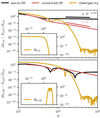 |
Fig. A.1. Convergence of the numerically computed eigenvalues Enl = E0, 0 (top) and Enl = E40, 6 (bottom) for three different discretization schemes. We find naive-FD, effective in the halo case, to show strongly degraded convergence properties under cylindrical symmetry. While the ad hoc corrected finite difference scheme (see text) recovers quadratic convergence, it is outperformed by the exponential convergence of the parity aware Chebyshev pseudospectral approach cheb-parity, which is the method of choice for this work. Insets: High-resolution (N = 4096) reference modes Rnl, the eigenvalue of which is used as Eref. |
Appendix B: WKB wave function coefficients
The task is to establish an equivalence between the DF defined real space density, cf. eq. (15):
 (B.1)
(B.1)
 (B.2)
(B.2)
and the wave-counterpart, cf. eq. (20):
 (B.3)
(B.3)
confined to:
 (B.4)
(B.4)
For isotropic, spherical systems this has been achieved in Yavetz et al. (2022) in the high-energy regime of the WKB solution for ψ — an idea which we follow. We also use the opportunity to emphasize a well-known, but sometimes overlooked, detail of the WKB formalism for radial Schrödinger equations that is of particular relevance at low angular momentum l.
What’s the WKB wave function un of bound state n in a regular, one-dimensional potential V(x)? If x ∈ ℝ, that is, defined on the entire real line, we have:
 (B.5a)
 (B.5b)
with normalization constant C and x1 < x as turning point, where the effective momentum satisfies p(x1) = 0.
One can show (Langer 1937; Berry & Almeida 1973) that this result is incorrect in the presence of a domain restricted to R ∈ ℝ+ and an effective potential that diverges as R → 0 — conditions both met for the radial Schrödinger equation eq. (A.1), but also in the spherically symmetric halo case 13. To be explicit, simply substituting eq. (B.4) in eq. (B.5b) for V(x), that is:
 (B.6)
(B.6)
yields wave functions eq. (B.5a) which do not faithfully approximate the solutions to eq. (A.1) (see Berry & Mount 1972, for a selection of problems).
In the cylindrical setting relevant here, Berry & Almeida (1973) show that transforming eq. (A.1) via:
 (B.7)
(B.7)
resolves all inconsistencies for states with l > 0. The effect of above transformation on the classical WKB result in eq. (B.5a) is summarized by the simple substitution l2 − 1/4 → l2 known as Langer’s correction (Langer 1937). The corrected, effective momentum reads:
 (B.8)
(B.8)
which reestablishes the classical form of the angular momentum barrier in eq. (B.2) if we identify the trivial mapping:
 (B.9)
(B.9)
Berry & Almeida (1973) show that s-waves (l = 0) do not follow a Langer-corrected version of eq. (B.5a). However, at high energies, Enl ≫ V, correct WKB s-waves are asymptotically equivalent to the l > 0 modes. As this is our regime of interest, it is correct to set unl as eq. (B.5a), but with the Langer corrected, effective momentum of eq. (B.8) for all l ≥ 0.
The normalization constant C follows from differentiation of the quantization condition ∫R1RdR′p(R′) = (n + 1/2)πℏ. One finds:
 (B.10)
Now, substituting eq. (B.8) into eq. (B.5a) and subsequently into eq. (B.3), converting the double sum into integrals via dLnl = ℏm−1dl and  , and approximating sin2(⋅)≃1/2 (permissible due to the fast oscillation of its argument) yields (under the assumption Enl ≫ V):
 (B.11)
By comparing with eq. (B.1), we arrive at:
 (B.12)
Above derivation is correct as long as ρDF and its associated DF are bounded. This is of course violated for β > 0, cf. eq. (16). No finite combination of eigenmodes will be able to reproduce a cuspy density profile as all of them are bounded. The best we can do in this scenario is to reproduce a cuspy ρDF up to some length scale of interest. This is achieved by an ad hoc change in the l = 0 WKB weights, if we set:
 (B.13)
Appendix C: Ellipsoidal collapse
We briefly summarize some mathematical details of the ellipsoidal collapse dynamics depicted in Fig. 9. An extensive discussion of the model is given in Bond & Myers (1996). Our notation follows Angrick & Bartelmann (2010).
We describe the evolution of the ellipsoid of mass M in its principal axis system. Let ai(a) be the scale factor in direction i, related to the physical size via  and density contrast δ = a3/(a1a2a3)−1. Each axis then evolves under the influence of the internal and external tidal forces and the cosmological background expansion. Choosing a flat ΛCDM background with E2(a) = ΩΛ + Ωma−3 and density parameters 1 = Ωm + ΩΛ, one finds:
![Mathematical equation: $$ \begin{aligned} 0&=\frac{\!\mathrm{d} ^2 a_i}{\!\mathrm{d} a^2} + \left[\frac{1}{a} + \frac{E^{\prime }(a)}{E(a)}\right]\frac{\!\mathrm{d} a_i}{\!\mathrm{d} a} + \left[\frac{3\Omega _m}{2a^5E^2(a)}C_i(a) - \frac{\Omega _\Lambda }{a^2E^2(a)}\right]a_i \;,\nonumber \\&\text{ with} \;\;\; C_i(a) = \frac{1+\delta (a)}{3} + \frac{b_i(a)}{2} + \lambda _\mathrm{ext,i} (a) \;. \end{aligned} $$](/articles/aa/full_html/2025/04/aa54232-25/aa54232-25-eq83.gif) (C.1)
(C.1)
Deviations from sphericity source tidal shears. Specifically,
![Mathematical equation: $$ \begin{aligned} b_i(a) = a_1(a)a_2(a)a_3(a)\int _0^\infty \frac{\!\mathrm{d} \tau }{\left[a_i^2(\tau )+1\right]\Pi _{k=1}^3\left[a_k^2(\tau )+1\right]^\frac{1}{2}} - \frac{2}{3} \;, \end{aligned} $$](/articles/aa/full_html/2025/04/aa54232-25/aa54232-25-eq84.gif) (C.2)
(C.2)
represents the internal tidal shear, whereas:
![Mathematical equation: $$ \begin{aligned} \lambda _\mathrm{ext,i} (a) = \frac{D(a)}{D(a_\mathrm{ini} } \left[\lambda _i(a_\mathrm{ini} ) - \frac{\delta (a_\mathrm{ini} )}{3}\right] \;, \end{aligned} $$](/articles/aa/full_html/2025/04/aa54232-25/aa54232-25-eq85.gif) (C.3)
(C.3)
models the external tidal shear contribution. Initial conditions for the scale factors ai at a = aini follow from Zeldovich’s approximation:
 (C.4a)
 (C.4b)
The eigenvalues of the Zeldovich deformation tensor λi relate to the shear ellipticity e and prolaticity p. Sheth et al. (2001) show that the most probable initial conditions have vanishing prolaticity, p = 0, so that:
 (C.5)
(C.5)
This concludes the specification of the initial conditions. What remains is a freeze out condition for each principal axis. In accordance with the condition of a quasi-virial filament state, cf. Sec. 2.2.1, we adopt the freeze-out approach of Angrick & Bartelmann (2010), which applies the tensor viral theorem (Binney & Tremaine 2008) to an ellipsoidal over density. One finds axis i to be virialized once the criterion:
 (C.6)
(C.6)
is met.
To compute the filament mass function, two ingredients are required: (i) the critical linear density, δec(e, z), at the redshift of filament formation, and (ii) a mapping from ellipticity e to filament mass M.
For the first step, we determine the unique initial overdensity δ(aini) for a given ellipticity e that results in the second axis to collapse at redshift z. To achieve this, we sweep over a broad range of ellipticities, optimize δ(aini) to meet the filament formation condition, and then extrapolate to z via the linear growth factor D(a).
For the ellipticity-to-filament mass mapping, we proceed as follows: We first map mass to the variance:
 (C.7)
(C.7)
of the density field smoothed on spatial scales R(M), and then map the variance to the ellipsoid’s ellipticity via the standard procedure outlined in Sheth et al. (2001). The linear matter power spectrum at z = 0 is set according to the analytical transfer function of Hu et al. (2000):
 (C.8)
(C.8)
where A = 0.179(m/1×10−22eV)−4/9Mpc. For the window function, W, a smooth-k filter is used (Du et al. 2024):
 (C.9)
(C.9)
with N-body calibrated values β = 9.10049 and cW = 2.1594.
These steps provide us with the mass-dependent (or, equivalently, the variance-dependent via eq. (C.7)) barrier shape:
 (C.10)
The excursion set formalism postulates that a randomly walking overdensity in σ2-space tracks the event of halo/filament formation (of mass M(σ2)) as the moment when its trajectory passes B(σ2, z) for the first time. The multiplicity function, fB(σ2), corresponds to the probability distribution of this event. Practically, it is found by carrying out Monte-Carlo simulations of the kind just described. For implementational convenience, however, we follow Zhang & Hui (2006), Benson et al. (2013), Du et al. (2016) and express fB(σ2) as the solution to the integral equation:
![Mathematical equation: $$ \begin{aligned} \int _0^{\sigma ^2}\text{ d}S\ f(S) \text{ erfc}\left[\frac{B(\sigma ^2,z) - B(S,z)}{\sqrt{2(\sigma ^2 - S)}}\right] =\text{ erfc}\left[\frac{B(\sigma ^2,z)}{\sqrt{2\sigma ^2}}\right]\;. \end{aligned} $$](/articles/aa/full_html/2025/04/aa54232-25/aa54232-25-eq94.gif) (C.11)
(C.11)
Eq. (33) then yields the FMF.
Appendix D: Single cylinder power spectrum
An advantage of our bottom-up filament model is that we have access to a semi-analytical version of the FDM wave function. Thus, we are able to compute Psingle(k) based off the eigenstate expansion directly rather than populating a high-resolution box with |ψ|2 and then treating it as a generic density of which k-space histogram is computed.
To compute eq. (42) we proceed as follows: Firstly, Fourier transform the normalized density uFDM, cf. eq. (38):
![Mathematical equation: $$ \begin{aligned} \hat{u}_\text{FDM}(\boldsymbol{k} \mid M)&= \mathcal{F} _{3D}\left[u_\text{FDM}(\boldsymbol{x} \mid M)\right]\nonumber \\&= \mathcal{F} _{3D}\left[M^{-1}\lambda \left(Z \mid L(M)\right)|\psi (R, \Phi )|^2\right] \\ &= M^{-1}\mathcal{F} _{1D}\left[\lambda \left(Z \mid L(M)\right)\right] \cdot \mathcal{F} _{2D}[|\psi (R, \Phi )|^2]. \end{aligned} $$](/articles/aa/full_html/2025/04/aa54232-25/aa54232-25-eq95.gif) (D.1)
(D.1)
Our choice of longitudinal density, eq. (37), was motivated by its rapidly decaying, simple Fourier transform,
![Mathematical equation: $$ \begin{aligned} \mathcal{F} _{1D}\left[\lambda \left(Z \mid L(M)\right)\right] = \frac{\sqrt{2/\pi } \exp \left(-\frac{k_Z^2}{4\Delta ^2}\right) \sin \left(\frac{k_ZL(M)}{2}\right)}{k}\;. \end{aligned} $$](/articles/aa/full_html/2025/04/aa54232-25/aa54232-25-eq96.gif) (D.2)
(D.2)
A simple closed form longitudinal spectrum reduces the problem of computing Psingle(k|M) to an effectively two-dimensional problem as  factorizes and its kZ-component does not need to be stored.
Secondly, to compute the cross-sectional contribution, ℱ2D[|ψ|2], we note that ψ is periodic in Φ. Thus, we may expand |ψ|2 and its Fourier transform as:
 = \sum _{m^{\prime }} g_{m^{\prime }}(k_R) e^{im^{\prime }\omega }\;. \end{aligned} $$](/articles/aa/full_html/2025/04/aa54232-25/aa54232-25-eq98.gif) (D.3)
(D.3)
Upon inserting the eigenstate ansatz for ψ and using orthonormality of the angular Fourier modes, we find:
 (D.4)
(D.4)
which is identical to the discrete autocorrelation of anlRnl(R) with angular momentum lag m and summed over all excitation numbers n. The coefficient function gm(kR) then follows from fm(R) via a mth-order Hankel transform ℍm (Baddour 2009):
\; \end{aligned} $$](/articles/aa/full_html/2025/04/aa54232-25/aa54232-25-eq100.gif) (D.5)
(D.5)
— conveniently implemented via the FFTLog algorithm (Talman 1978; Hamilton 2000) applied to each mode. This also fixes the values of R to a log-uniform grid on which eq. (D.4) has to be evaluated.
Lastly, with  in cylindrical coordinates k = (kR, kZ, ω)⊺ at hand, we perform a spherical average of the squared modulus to arrive at the isotropic, single cylinder power spectrum:
 (D.6)
(D.6)
We repeat the outlined procedure for multiple wave function coefficient phase realizations i and then average all Psingle, i(k) to arrive at an ensemble estimate. The solid lines in both panels of Fig. 12 show this ensemble average.
All Figures
|
Fig. 1. Top: Cross section of a steady-state FDM filament with FDM mass m = 2 × 10⁻²² eV at redshift z = 4. The interference is constructed as a post-processing step for an interference-free background density which may be provided by an analytical model (this work) or DM simulations (future work). Bottom: Volume rendering of a toy filament obtained by extruding above cross section along a straight filament spine. Section 2 models FDM filaments as infinitely long versions of such extrusions. In Sect. 3 we find a physically-sound extrusion length for our 2D model via ellipsoidal collapse considerations. |
| In the text | |
|
Fig. 2. Top: Gravitational potential sourced by the axial-symmetric contribution ⟨|ψ|2⟩Φ = ⟨|ψ|2⟩ of the wave function depicted in Fig. 1. Bottom: Relative importance of the potential perturbation sourced by the interference term alone. Neglecting the latter in the computation of the total potential in Eq. (1b) only incurs 𝒪(1 − 10%) errors. |
| In the text | |
|
Fig. 3. Radial filament densities obtained from Eq. (12) (solid lines) and the solution of the inverse problem of Eq. (17) (dashed lines), i.e., the density implied by the DF. Vertical lines depict the fit radius R99 within which 99% of the total line mass μ are contained. |
| In the text | |
|
Fig. 4. Recovered DFs for the densities depicted in Fig. 3 for various values of the specific angular momentum L = l × ℏm−1. Note that (i) we only show L = 0 for β = 0 as the DF is uniform in L for isotropic conditions, cf. Eq. (16), (ii) energies are bound from below by Ec(L), the energy of a circular orbit defined as the minimum of the effective potential V(R)+L2/2a2R2 and (iii) both DFs recover a Boltzmann-like, exponential behavior in E. We emphasize that this functional behavior is not imposed by our inversion of Eq. (17). |
| In the text | |
|
Fig. 5. Subset of the eigenstate library for m = 2 × 10⁻²² eV and β = 0 at redshift z = 4. The total library for this parameter combination contains J = 746 states. As is the case for halos, the small radii behavior of radial eigenstates is determined by the angular momentum Rnl(R)∼Rl, while n ∈ ℕ is equivalent to the number of nodes in Rnl. For fixed l, the maximal n is set by Enl < V(R99) and lmax follows from min(Veff, ψ) < V(R99). |
| In the text | |
|
Fig. 6. Comparison of various coefficient estimators |anl|2 for m = 2 × 10⁻²² eV with β = 0 (top) and β = 0.5 (bottom) at z = 4. While the WKB result, Eq. (22), reproduces the background density well without any optimization, the posterior modes adaptive LASSO and l1-Poisson show identical accuracy while reducing the number of involved modes significantly. |
| In the text | |
|
Fig. 7. Top row: Wave function density |ψ|2, i.e., the static terms shown in Fig. 6 and the interference term, as a function of the anisotropy parameter. Bottom row: Interference modulates the density comparable to the magnitude of the background density leading to a concentric ring pattern for the radially biased case (right column) and a more mixed interference fringe configuration under isotropic conditions (left column). |
| In the text | |
|
Fig. 8. Reconstructed FDM interference as a function of axion mass for an isotropic background density at redshift z = 4. First row: FDM density, |ψ|2, as in Eq. (5), i.e., including both the time static and interference term. Second row: The interference term relative to static background density. Strong, 𝒪(1), interference features are observable both in the radial and azimuthal direction, indicative of an isotropic, β = 0, background density. Third row: The wave function phase Arg[ψ]. Quantized vortices (red circles, shown only for the left hand column), another feature unique for FDM, correspond to 2π discontinuities in the phase function, or as described in the main text, places of nonzero vorticity, Eq. (30). |
| In the text | |
|
Fig. 9. Example of ellipsoidal collapse in a ΛCDM background for a homogeneous ellipsoid with mass M = 5 × 10⁹ M⊙ h−1. The equation of motion, Eq. (C.1), preserves the homogeneity of the initial conditions and it is thus sufficient to observe the evolution of the axis scale factors ai(a). After an initial expansion, each axis turns around, contracts and freezes out according to the steady-state tensor virial theorem, Eq. (C.6). The subsequent evolution is fixed to ensure a constant comoving axis size Ri = ai(a)Rini/a. We identify a filament as an object with two frozen axes – in the depicted scenario realized at z = 4. The residual triaxiality, i.e., the mismatch between the yellow and red lines at large a, is ignored for the construction of our filament population. |
| In the text | |
|
Fig. 10. Filament mass function (FMF) for various FDM masses at redshift z = 4. The suppression in the linear FDM power spectrum translates to a power suppression for filament masses. For filament masses M > 3 × 10⁹ h−1 M⊙, all considered FDM cases are indistinguishable from CDM and it is in this regime in which we sample the FMF in order to guarantee the same overall number density and thus same significance of interference effects measured in the correlation functions discussed in Sect. 3. |
| In the text | |
|
Fig. 11. Volume rendering of the idealized FDM filament sample for m22 = 1 in a periodic, comoving box of L = 2 h−1 Mpc at z = 4, generated by sampling the FMF in Fig. 10 for masses M > 3 × 10⁹ h−1 M⊙. The same realization is shown from three different viewing angles. The characteristic filament length is ≃1 − 2 h−1 Mpc. The random iid placement of the cylinders neglects any filament-filament cross-correlations encoded in the cosmic web. Consequently, one expects the power spectrum of the box shown to be identical to the one-filament term in Eq. (41). This is supported by Fig. 12 which compares the spectrum of the domain depicted in this Figure (dashed, yellow) with the stacked spectra following from Eq. (41) (solid, blue). |
| In the text | |
|
Fig. 12. Three-dimensional filament matter power spectra of the interference-free CDM background and the reconstructed FDM density for a selection of FDM masses at z = 4. Top: Single filament spectrum, Psingle(k ∣ M), for an example filament of total mass M = 5 × 10⁹ h−1 M⊙. One finds all FDM spectra to be compatible with CDM down to the spatial extent of the ground state, Rgs ≡ ⟨ψ0|R|ψ0⟩ (vertical, dashed line) – effectively the characteristic scale of the cylinder. Once sufficiently small scales inside the filament are probed, the interference contribution to |ψ|2 enhances the two point density correlation and boosts Psingle(k ∣ M) above the CDM baseline. Note that for larger m22: (i) Psingle(k ∣ M) detaches later from the CDM baseline, (ii) the boost is shallower but (iii) extends to higher k until the suppression scale kcut ∝ m is reached (vertical, solid lines). Bottom: One-filament term P1f(k) – a stacked version of many Psingle(k ∣ M), weighted according to the FMF in Fig. 10. We limit the filament population to the mass window M ∈ [3×10⁹, 3×10¹⁰] h−1 M⊙ and compute the one filament term either directly from the semi-analytical expression of the wave function developed in Appendix D (solid, blue) or by populating a box as shown in Fig. 11 (dashed, yellow). All quantitative observations made for the single cylinder case translate to P1f(k) after a FMF-weighted average according to Eq. (45), i.e., Rgs → ⟨Rgs⟩FMF (vertical, dashed lines) and kcut → ⟨kcut⟩FMF (vertical, solid lines). |
| In the text | |
|
Fig. A.1. Convergence of the numerically computed eigenvalues Enl = E0, 0 (top) and Enl = E40, 6 (bottom) for three different discretization schemes. We find naive-FD, effective in the halo case, to show strongly degraded convergence properties under cylindrical symmetry. While the ad hoc corrected finite difference scheme (see text) recovers quadratic convergence, it is outperformed by the exponential convergence of the parity aware Chebyshev pseudospectral approach cheb-parity, which is the method of choice for this work. Insets: High-resolution (N = 4096) reference modes Rnl, the eigenvalue of which is used as Eref. |
| In the text | |
Current usage metrics show cumulative count of Article Views (full-text article views including HTML views, PDF and ePub downloads, according to the available data) and Abstracts Views on Vision4Press platform.
Data correspond to usage on the plateform after 2015. The current usage metrics is available 48-96 hours after online publication and is updated daily on week days.
Initial download of the metrics may take a while.