© S. T. H. Hartman et al. 2022

1. Introduction

Unveiling the fundamental nature of dark matter (DM) – the dominant matter component of our Universe – has been one of the ultimate goals of physics for many decades. Although its particle identity has remained elusive, the collisionless and cold DM (CDM) paradigm, along with a cosmological constant and inflationary initial conditions, has proven extremely successful at explaining a wide range of observables, and is known as the ΛCDM model (Davis et al. 1985; Percival et al. 2001; Tegmark et al. 2004; Trujillo-Gomez et al. 2011; Vogelsberger et al. 2014; Planck Collaboration XIII 2016; Riess et al. 2016; Cyburt et al. 2016). Nevertheless, the quest for a complete theory of DM has spawned numerous expanded models, many of which aim to reproduce the success of CDM while attempting to fix discrepancies between ΛCDM and observations, finding physics beyond the standard model of particle physics (SM), or both.

Some of the tensions in ΛCDM are related to the formation and shape of small-scale structures. CDM, due to its cold and collisionless nature, is very efficient at forming structure at all scales. For instance, N-body simulations predict CDM halos to follow the universal Navarro-Frenk-White (NFW) profile (Navarro et al. 1996, 1997), which diverges near the center as ρ(r)∼r⁻¹, whereas measurements instead indicate the central regions of DM profiles of low-mass halos to be flatter, or rather, that low-mass halos are cored rather than cuspy. Furthermore, ΛCDM predicts a large number of low-mass halos, as well as massive subhalos that should be too big to fail at forming stars, yet these are largely absent in our galactic neighborhood. These issues of ΛCDM, known as the “cusp-core”, “missing-halo”, and “too-big-to-fail” problems, respectively, might be due to limitations in accurately modeling baryonic physics and processes that are too small to be resolved in large-scale simulations (see Weinberg et al. 2015; Del Popolo & Le Delliou 2017; Bullock & Boylan-Kolchin 2017, and references therein for further discussion on these small-scale discrepancies in ΛCDM). Alternatively, the solution might lie in the dark sector.

A popular class of DM models beyond CDM involve ultra-light scalar, or pseudo-scalar, particles that have a sufficiently small mass to exhibit wave-like behaviour on astrophysical scales. The free-field case, termed Fuzzy DM (FDM; Dine & Fischler 1983; Preskill et al. 1983; Hu et al. 2000; Marsh 2016; Hui et al. 2017), with masses as low as 10⁻²² eV, have large de Broglie wavelengths λ_dB = 1/mv and produce solitonic cores of order 1 kpc at the centers of DM halos. Unlike CDM, which clusters on all scales, FDM suppresses small-scale structure because of an effective Jeans’ length due to the large de Broglie wavelength. Furthermore, FDM produces interference patterns in its density distribution, which is a very distinct feature of FDM compared to CDM and other DM models, such as warm DM. However, a recent bound on the FDM mass from the Lyman-alpha forest constrains it to m > 2 × 10⁻²⁰ eV, and therefore seems to rule out the canonical mass-range generally considered to be needed to solve the small-scale problems of ΛCDM (Rogers & Peiris 2021).

Another kind of ultra-light DM are scalar fields with interactions. These can vary in complexity, from single-field DM with self-interactions (Lee & Koh 1996; Peebles 2000; Goodman 2000; Arbey et al. 2002, 2003; Böhmer & Harko 2007; Chavanis 2011; Rindler-Daller & Shapiro 2012), to multi-field DM with non-trivial couplings that give rise to exotic properties (Matos et al. 2000; Bettoni et al. 2014; Berezhiani & Khoury 2015; Khoury 2016; Ferreira et al. 2019), though a common feature among these models is for the interactions to give rise to a fluid pressure that produces halo cores. The simplest scenario is single-field DM with quartic self-interactions and a negligible de Broglie wavelength, which, along with FDM, is often referred to as Bose-Einstein condensed DM, because they can be regarded as the zero-temperature limit of a boson gas, which in mean-field theory is described by a classical field (Pitaevskii & Stringari 2016). The term superfluid DM is also frequently used due to the close relationship between Bose-Einstein condensates and superfluidity, though in this work we will instead use “self-interacting Bose-Einstein condensed” (SIBEC) DM, in an effort to emphasize the importance of the self-interactions on the dynamics of the scalar field.

The non-linear structure of SIBEC-DM has largely been investigated near hydrostatic equilibrium, which finds SIBEC-DM halo cores to be independent of the total halo mass and core density. Fitting SIBEC-DM to nearby galaxies reproduces the observed rotation curves for core radii around 1 kpc and larger (Zhang et al. 2018; Crăciun & Harko 2020). However, to obtain more realistic SIBEC-DM halo profiles from cosmological structure formation, which are expected transition to into the NFW profile outside the cores, one needs to go beyond hydrostatic considerations and use numerical simulations, though some challenges arise in such an endeavor. For instance, the equation of motion for non-relativistic scalar fields, the non-linear Schrödinger equation (NLSE), is very computationally demanding to solve, even in the FDM-limit where the de Broglie wavelength is of astrophysical scale. For SIBEC-DM, where λ_dB is much smaller, but still needs to be resolved, the NLSE is even more computationally demanding. Simply setting the terms that describe the dynamics at λ_dB-scales to zero, which works in the hydrostatic case, does not work in non-linear simulations, as they play an important role in regularizing discontinuities and keeping the numerical solution well-behaved. A scheme that somehow incorporates the de Broglie scale without actually needing to resolve it is therefore desired, and was recently employed by Dawoodbhoy et al. (2021) and Shapiro et al. (2021). They used a hydrodynamic formulation of the NLSE that incorporates the dynamics on the de Broglie scale as an effective thermal pressure, and performed 1D simulations of collapsing spherical overdensities of SIBEC-DM. They found that in a non-cosmological setting, SIBEC-DM halos with cores of order 1 kpc provide a solution to the small-scale issues of the standard model. In fact, they found SIBEC-DM to provide a better solution to both the too-big-to-fail and cusp-core problems than FDM, which struggles to fix these two issues at the same time (Robles et al. 2019). Moving to a cosmological setting, on the other hand, results in an overly large suppression of the formation of small-scale halos for these same core radii. The cores therefore have to be smaller than what is needed to provide a solution to, for instance, the core-cusp issue, in order to be compatible with the halo mass function. A similar conclusion was drawn by Hartman et al. (2022) using large-scale observables, albeit to a much lesser degree. Exploring the formation of non-linear structure in a universe with SIBEC-DM and investigating the properties of SIBEC-DM halos is nevertheless a worthwhile endeavor in the effort to further understand the rich phenomenology that is found in scalar field DM models. In this paper we therefore build on the work of Dawoodbhoy et al. (2021) and Shapiro et al. (2021) by implementing the de Broglie-smoothed hydrodynamic formulation of SIBEC-DM into a modified version of the RAMSES code (Teyssier 2002). This code is then used to perform fully 3D cosmological simulations to explore the formation of SIBEC-DM structures and their non-linear dynamics. The paper is structured as follows: In Sect. 2 the basic theoretical framework for modelling scalar field DM is reviewed, along with the smoothing procedure used to derive the hydrodynamic approximation for SIBEC-DM. In Sect. 3 the numerical aspects of this paper are discussed, including a brief description of how the RAMSES code works, the initial setup of the SIBEC-DM fluid, and a discussion of the limitations of the simulations. Our main results are presented and discussed in Sect. 4, with final conclusions in Sect. 5. We use, for the most part, natural units.

2. Theory of self-interacting Bose-Einstein condensates dark matter

Ultra-light scalar DM can be described by a classical field theory, and one of the simplest realizations is the Lagrangian for a complex scalar field Ψ with self-interactions (Li et al. 2014),

$$\begin{array}{c}\hfill \mathcal{L}=\frac{1}{2m}{g}_{\mu \nu }{\partial }^{\mu }{\mathrm{\Psi }}^{\ast }{\partial }^{\nu }\mathrm{\Psi }-\frac{1}{2}{m|\mathrm{\Psi }|}^2-\frac{1}{2}g{|\mathrm{\Psi }|}^4,\end{array}$$(1)

where m is the mass of the scalar field, and g is the coupling parameter for the self-interaction. In the early universe, where DM is much denser and the self-interaction of the scalar field dominates the energy density, the averaged pressure and energy of the field behave as radiation (Matos & Arturo Ureña-López 2001; Li et al. 2014). As the universe expands and becomes more diluted, the interaction energy eventually becomes smaller than the rest energy of the field, and it ceases to be radiation-like. In this non-relativistic phase we can define a new field, Ψ = ψe^−imt, whose dynamics are given by the NLSE (Ferreira 2021),

$$\begin{array}{c}\hfill i\frac{\partial \psi }{\partial t}=[\frac{-{\mathrm{\nabla }}^2}{2m}+V]\psi ,\end{array}$$(2)

where V = g|ψ|² + mϕ includes two-body contact interactions and the gravitational potential ϕ. The NLSE can be reformulated in a hydrodynamical form by substituting for the wavefunction

$$\begin{array}{c}\hfill \psi =\sqrt{n}{e}^{\mathit{iS}}=\sqrt{\frac{\rho }{m}}{e}^{\mathit{iS}},\end{array}$$(3)

where n is the particle number density, ρ = mn the mass density, and the velocity field is defined by v = ∇S/m. This gives the Madelung equations (Madelung 1926),

$$\begin{array}{cc}& \frac{\partial \rho }{\partial t}+\mathbf{\nabla }·(\rho \mathit{v})=0,\hfill \end{array}$$(4)

$$\begin{array}{cc}& \frac{\partial \mathit{v}}{\partial t}+(\mathit{v}·\mathbf{\nabla })\mathit{v}+\mathbf{\nabla }(\frac{g\rho }{m^2}-\frac{1}{2m^2}\frac{{\mathrm{\nabla }}^2\sqrt{\rho }}{\sqrt{\rho }}+\varphi )=\mathbf{0},\hfill \end{array}$$(5)

which are readily recognizable as an equation for mass conservation and a variant of the momentum equation. The largest difference from standard hydrodynamics is the absence of an energy equation, the presence of a self-interaction pressure

$$\begin{array}{c}\hfill P_{\mathrm{SI}}=\frac{g{\rho }^2}{2m^2},\end{array}$$(6)

and a so-called quantum potential

$$\begin{array}{c}\hfill Q=-\frac{1}{2m^2}\frac{{\mathrm{\nabla }}^2\sqrt{\rho }}{\sqrt{\rho }}·\end{array}$$(7)

The phenomenology of ultra-light DM depends crucially on whether the interaction pressure or the quantum potential dominates. This becomes apparent when considering halo properties of ultra-light DM at equilibrium. In the FDM-limit, the de Broglie wavelength of the ultra-light DM particles is much larger than the Jeans’ length of the self-interaction and is of astrophysical size, such that small-scale structure is stabilized against collapse due to the formation of solitonic cores for masses m ≲ 10⁻²¹. The core radii of FDM halos at hydrostatic equilibrium are approximately (Membrado et al. 1989)

$$\begin{array}{c}\hfill R_{\mathrm{FDM}}=\frac{10}{GM{m}^2},\end{array}$$(8)

where M is the total mass of the halo. The opposite limit Q ≪ P_SI/ρ, which is the case we refer to as SIBEC-DM, but is also known as the Thomas-Fermi approximation, results in the hydrostatic density profile (Goodman 2000)

$$\begin{array}{c}\hfill \rho (r)={\rho }_0\frac{sin(Ar)}{\mathit{Ar}},\end{array}$$(9)

where $A=\sqrt{4\pi G{m}^2/g}$, and goes to zero at

$$\begin{array}{c}\hfill r=R_{\mathrm{c}}=\sqrt{\frac{g\pi }{4G{m}^2}}·\end{array}$$(10)

The soliton cores of massive FDM halos are smaller than low-mass halos, a feature confirmed by simulations (Chan et al. 2022), whereas the core radius R_c of halos in the Thomas-Fermi limit is independent of the total halo mass and central density, depending only on the combination g/m².

Both the NLSE and its hydrodynamic Madelung formulation are widely used to study ultra-light DM across a wide range of scales, from the properties of low-mass halos and galaxies (Membrado et al. 1989; Goodman 2000; Böhmer & Harko 2007; Chavanis 2011; Chavanis & Delfini 2011; Rindler-Daller & Shapiro 2014; Hui et al. 2017; Zhang et al. 2018; Berezhiani et al. 2019; Crăciun & Harko 2020; Lancaster et al. 2020) to large-scale simulations (Schive et al. 2014a,b; Schwabe et al. 2016; Mocz et al. 2017, 2018; Veltmaat et al. 2018; Nori & Baldi 2018; Mina et al. 2020, 2022; Nori & Baldi 2021; May & Springel 2021). However, only the FDM-limit has been thoroughly investigated using fully 3D cosmological simulations. No corresponding work has so far been carried out in the Thomas-Fermi limit, in part due to a number of challenges in simulating this kind of system. The hydrodynamic equations obtained by neglecting the quantum potential appear equivalent to regular hydrodynamics with an adiabatic index γ = 2, such that it seems standard numerical schemes should work, but as shock fronts and discontinuities arise, the Thomas-Fermi approximation breaks down and the full equations are needed. However, both the NLSE and Madelung equations are computationally demanding to solve due to the high resolution needed to resolve the scales on which the quantum potential operates. This is already a challenge in FDM simulations, but even more so for SIBEC-DM where the characteristic scale of Q is much smaller than the scales of interest given by the interaction pressure, λ_dB ≪ R_c.

2.1. Smoothed SIBEC hydrodynamics

An alternative hydrodynamic approximation of SIBEC-DM that includes the effect of the quantum potential without actually needing to resolve λ_dB was recently used by Dawoodbhoy et al. (2021) and Shapiro et al. (2021). It involves using a smoothed phase space representation of the wavefunction, known as the Husimi representation (Husimi 1940), which is obtained by essentially smoothing over ψ with a Gaussian window function of width η and Fourier transforming;

$$\begin{array}{c}\hfill \mathrm{\Psi }(\mathit{x},\mathit{p},t)={\displaystyle \int }\frac{{\mathrm{d}}^{3}y}{{(2\pi )}^{3/2}}\frac{e^{-{(\mathit{x}-\mathit{y})}^2/2{\eta }^2}}{{(\eta \sqrt{\pi })}^{3/2}}\psi (\mathit{y},t)e^{-i\mathit{p}·(\mathit{y}-\mathit{x}/2)}.\end{array}$$(11)

Defining the phase space distribution function

$$\begin{array}{c}\hfill \mathcal{F}(\mathit{x},\mathit{p},t)={|\mathrm{\Psi }(\mathit{x},\mathit{p},t)|}^2,\end{array}$$(12)

and computing the derivative ∂ℱ/∂t, using the NLSE i∂ψ/∂t = [ − ∇²/2m + V]ψ, and smoothing over scales larger than the de Broglie wavelength λ_dB ≪ η, gives an approximate equation of motion that is of the same form as the collisionless Boltzmann equation (Skodje et al. 1989; Widrow & Kaiser 1993);

$$\begin{array}{c}\hfill \frac{\mathrm{d}\mathcal{F}}{\mathrm{d}t}=\frac{\partial \mathcal{F}}{\partial t}+\frac{p_i}{m}\frac{\partial \mathcal{F}}{\partial x_i}-\frac{\partial V}{\partial x_i}\frac{\partial \mathcal{F}}{\partial p_i}=0.\end{array}$$(13)

The gravitational potential and the mean-field potential due to self-interactions in V are now given by the smoothed density field, which is obtained from ℱ in the same way as from a standard phase space distribution function,

$$\begin{array}{c}\hfill \rho (\mathit{x},t)=m{\displaystyle \int }{\mathrm{d}}^{3}p\mathcal{F}(\mathit{x},\mathit{p},t)={\displaystyle \int }{\mathrm{d}}^{3}y\frac{e^{-{(\mathit{x}-\mathit{y})}^2/{\eta }^2}}{{(\eta \sqrt{\pi })}^3}m{|\psi (\mathit{y},t)|}^2.\end{array}$$(14)

Following Dawoodbhoy et al. (2021), the hydrodynamic equations for SIBEC-DM in this approximation are obtained from the zeroth, first, and second moments of Eq. (13), and it is assumed that the phase space distribution function is isotropic around its mean momentum ⟨p⟩, that is, that ℱ(x, p, t) is skewless in p. This ansatz is supported by the results of Veltmaat et al. (2018), who performed 3D simulations of FDM halo mergers using the NLSE and found the velocity distribution of plane waves inside the virial radius to be Maxwellian. Before the growth of non-linear structures, and outside of halos, such as in regions that have not undergone violent relaxation and shell crossing, the assumption of skewlessness in ℱ may not hold true. On the other hand, the fluid is supersonic and ballistic in these regions, as well as dominated by the interaction pressure, so it should not matter in these situations. During mergers, however, the skewless assumption might also break down and have significant implications if the merging halos have large plane-wave velocity dispersions. We nevertheless use this assumption throughout our simulations. The resulting equations are

$$\begin{array}{cc}& \frac{\partial \rho }{\partial t}+\mathbf{\nabla }·\mathit{j}=0,\hfill \end{array}$$(15)

$$\begin{array}{cc}& \frac{\partial \mathit{j}}{\partial t}+\mathbf{\nabla }(P+P_{\mathrm{SI}})+\rho (\mathit{v}·\mathbf{\nabla })\mathit{v}+\mathit{v}(\mathbf{\nabla }·\rho \mathit{v})=-\rho \mathbf{\nabla }\varphi ,\hfill \end{array}$$(16)

$$\begin{array}{cc}& \frac{\partial E}{\partial t}+\mathbf{\nabla }·[(E+P+P_{\mathrm{SI}})\mathit{v}]=-\mathit{j}·\mathbf{\nabla }\varphi .\hfill \end{array}$$(17)

There are two major changes in the above hydrodynamic description of BECs compared to the Madelung equations; first, there is no quantum potential; and second, there is an energy equation in addition to the continuity and momentum equations, with the total energy given by

$$\begin{array}{c}\hfill E=\frac{1}{2}\rho v^2+U+U_{\mathrm{SI}},\end{array}$$(18)

where $P=\frac{2}{3}U$ and P_SI = U_SI. In fact, the small-scale dynamics of the Madelung equations driven by the quantum potential, after smoothing over scales larger than the de Broglie wavelength, behave effectively as an ideal gas with adiabatic index γ = 5/3, with an additional pressure and internal energy due to the self-interactions. The fluid variables, such as the fluid density and momentum, and the effective thermal internal energy and pressure, are defined in the same way as in classical statistical mechanics (Huang 1987), but using the smoothed phase space representation of the wavefunction rather than a phase space distribution function of classical point particles;

$$\begin{array}{cc}& n(\mathit{x},t)={\displaystyle \int }{\mathrm{d}}^{3}p\mathcal{F}(\mathit{x},\mathit{p},t),\hfill \end{array}$$(19)

$$\begin{array}{cc}& \mathit{j}(\mathit{x},t)=n\mathit{p}={\displaystyle \int }{\mathrm{d}}^{3}p\mathit{p}\mathcal{F}(\mathit{x},\mathit{p},t),\hfill \end{array}$$(20)

$$\begin{array}{cc}& P(\mathit{x},t)={\displaystyle \int }{\mathrm{d}}^{3}p\frac{{|\mathit{p}-\mathit{p}|}^2}{3m}\mathcal{F}(\mathit{x},\mathit{p},t),\hfill \end{array}$$(21)

$$\begin{array}{cc}& U(\mathit{x},t)={\displaystyle \int }{\mathrm{d}}^{3}p\frac{{|\mathit{p}-\mathit{p}|}^2}{2m}\mathcal{F}(\mathit{x},\mathit{p},t),\hfill \end{array}$$(22)

$$\begin{array}{cc}& E(\mathit{x},t)=U_{\mathrm{SI}}+{\displaystyle \int }{\mathrm{d}}^{3}p\frac{p^2}{2m}\mathcal{F}(\mathit{x},\mathit{p},t).\hfill \end{array}$$(23)

In the following, we will sometimes refer to the “effective thermal” energy and pressure as simply “thermal”.

2.2. Supercomoving hydrodynamics

Now that we have a set of fluid equations for SIBEC-DM, we would like to apply these to the growth of structure in a cosmological setting. A convenient set of coordinates for this purpose are the so-called supercomoving coordinates (Martel & Shapiro 1998), which uses the following change of variables in the case of a flat universe dominated by matter and a cosmological constant;

$$\begin{array}{cc}\hfill \stackrel{\sim }{\mathit{x}}& =\frac{1}{a}\frac{\mathit{x}}{L},\mathrm{d}\stackrel{\sim }{t}=H_0\frac{\mathrm{d}t}{a^2},\stackrel{\sim }{\rho }=a^3\frac{\rho }{{\mathrm{\Omega }}_{\mathrm{m}0}{\rho }_{\mathrm{c}0}},\hfill \\ \hfill \stackrel{\sim }{\mathit{u}}& =a\frac{\mathit{u}}{H_{0}L},\stackrel{\sim }{P}=a^5\frac{P}{{\mathrm{\Omega }}_{\mathrm{m}0}{\rho }_{\mathrm{c}0}{H}_0^2{L}^2},\hfill \\ \hfill \stackrel{\sim }{m}& =m{H}_{0}L,\stackrel{\sim }{g}=g\frac{{\mathrm{\Omega }}_{\mathrm{m}0}{\rho }_{\mathrm{c}0}}{a},\hfill \end{array}$$(24)

where the peculiar motion u = v − Hr is introduced. L is a free length scale parameter, Ω_m0 is the fraction of matter today, and ρ_c0 the critical energy density today. In these coordinates, the fluid equations in an expanding universe are on a similar form as the standard equations on a static background;

$$\begin{array}{cc}& \frac{\partial \stackrel{\sim }{\rho }}{\partial \stackrel{\sim }{t}}+\stackrel{\sim }{\mathbf{\nabla }}·\stackrel{\sim }{\mathit{j}}=0,\hfill \end{array}$$(25)

$$\begin{array}{cc}& \frac{\partial \stackrel{\sim }{\mathit{j}}}{\partial \stackrel{\sim }{t}}+\stackrel{\sim }{\mathbf{\nabla }}({\stackrel{\sim }{P}}_{\mathrm{tot}})+\stackrel{\sim }{\rho }(\stackrel{\sim }{\mathit{u}}·\stackrel{\sim }{\mathbf{\nabla }})\stackrel{\sim }{\mathit{u}}+\stackrel{\sim }{\mathit{u}}(\stackrel{\sim }{\mathbf{\nabla }}·\stackrel{\sim }{\rho }\stackrel{\sim }{\mathit{u}})=-\stackrel{\sim }{\rho }\stackrel{\sim }{\mathbf{\nabla }}\stackrel{\sim }{\varphi },\hfill \end{array}$$(26)

$$\begin{array}{cc}& \frac{\partial \stackrel{\sim }{E}}{\partial \stackrel{\sim }{t}}+\stackrel{\sim }{\mathbf{\nabla }}·[(\stackrel{\sim }{E}+{\stackrel{\sim }{P}}_{\mathrm{tot}})\stackrel{\sim }{\mathit{u}}]+\mathcal{H}(3{\stackrel{\sim }{P}}_{\mathrm{tot}}-2{\stackrel{\sim }{U}}_{\mathrm{tot}})=-\stackrel{\sim }{\mathit{j}}·\stackrel{\sim }{\mathbf{\nabla }}\stackrel{\sim }{\varphi }.\hfill \end{array}$$(27)

where ${\stackrel{\sim }{P}}_{\mathrm{tot}}=\stackrel{\sim }{P}+{\stackrel{\sim }{P}}_{\mathrm{SI}}$ and ${\stackrel{\sim }{U}}_{\mathrm{tot}}=\stackrel{\sim }{U}+{\stackrel{\sim }{U}}_{\mathrm{SI}}$. The supercomoving Hubble parameter is given by $\mathcal{H}=a^{-1}\mathrm{d}a/\mathrm{d}\stackrel{\sim }{t}$, the gravitational potential by

$$\begin{array}{c}\hfill {\stackrel{\sim }{\mathrm{\nabla }}}^2\stackrel{\sim }{\varphi }=\frac{3}{2}a{\mathrm{\Omega }}_{\mathrm{m}}(\stackrel{\sim }{\rho }-1),\end{array}$$(28)

and expressions for the energies, pressures, and so on, are the same as before, but with supercomoving quantities. A notable difference from regular hydrodynamics is the presence of the Hubble drag in the supercomoving energy equation, which vanishes for the ideal gas pressure with γ = 5/3, but not for the self-interaction pressure.

3. Numerical implementation

A modified version of RAMSES (Teyssier 2002) is used to simulate the formation of structure of SIBEC-DM in a cosmological setting. The halo catalogs are obtained with Amiga’s Halo Finder (AHF; Gill et al. 2004; Knollmann & Knebe 2009), and plots of simulation snapshots are made using the python package YT (Turk et al. 2010). RAMSES is a grid based code that uses adaptive mesh refinement (AMR) to focus computational resources through a hierarchy of nested grids, increasing the local resolution in regions of interest. This is done by recursively splitting individual cells into 2^N smaller cells, where N is the dimensionality, until a set of refinement criteria are satisfied, doubling the spatial resolution at each new level of refinement. For a box of length L, the cell length at refinement level l is Δx^l = L/2^l.

RAMSES was originally developed for cosmological simulations of the formation and evolution of structure at both large and small scales, using an N-body particle-mesh code for CDM, with which the phase space distribution of DM is sampled through a computationally tractable number of collisionless macroparticles. The gravitational forces acting on these macroparticles are obtained by projecting the DM mass onto the AMR grid and solving the Poisson equation. RAMSES also includes code for studying gas dynamics, using the grid and a Godunov scheme to solve the hydrodynamic equations in supercomoving coordinates. It is this latter part of RAMSES that has been modified in order to solve the SIBEC-DM hydrodynamic equations, and we use a second-order Godunov scheme with the Rusanov flux (an HLLE Riemann solver) and the van Leer slope limiter to compute the flux at the cell interfaces (Toro 2006). The Rusanov flux is computed using the conservative variables $\stackrel{\sim }{\rho }$, $\stackrel{\sim }{\mathit{j}}$, and $\stackrel{\sim }{E}$, and Eqs. (25)–(27), while the second-order MUSCL-Hancock and slope limiting step is done using the primitive variables $\stackrel{\sim }{\rho }$, $\stackrel{\sim }{\mathit{u}}$, and $\stackrel{\sim }{P}$ (the thermal pressure).

A 3D test of the collapse of a spherically symmetric overdensity at two different grid resolutions (refinement levels 7 to 11, and 8 to 12) are included in Fig. 1. A periodic box of size L = 50 kpc was used, with the initial density ρ(r) = ρ₀[1 + e^−(r/R)2], where R = 5 kpc and ρ₀ = 0.3ρ_c0. The initial thermal pressure was ζ = P/P_SI = 10⁻¹, and the simulations were run until 3 t_dyn, where $t_{\mathrm{dyn}}=\sqrt{3/8\pi G{\rho }_0}$ is the dynamical timescale of the initial overdensity. The energy density profiles, with

$$\begin{array}{c}\hfill W=-\frac{GM(<r)\rho }{r}·\end{array}$$(29)

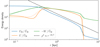Fig. 1. Self-interaction energy density USI, thermal energy density U, and gravitational potential energy density W of the spherically symmetric test halo with Rc = 1 kpc, relative to the interaction energy of the initial background ${\overline{U}}_{\mathrm{SI}}$. The result of the simulation with refinement levels 8 to 12 are shown in solid, while 7 to 11 is shown in dotted. The 3D simulation reproduces the 1D results of Ahn & Shapiro (2005) and Dawoodbhoy et al. (2021), in particular the large thermal energy in the wake of the accretion shock, its sharp decrease to below the self-interaction energy inside the core, and the fit USI ∝ ρ2 ∝ r−24/7 in the envelope.

agrees with the results of the 1D simulations of Ahn & Shapiro (2005) and Dawoodbhoy et al. (2021), in particular the large thermal energy in the wake of the accretion shock, its sharp decrease to below the self-interaction energy inside the core, and the fit ρ ∝ r^−12/7 in the envelope, which gives U_SI ∝ ρ² ∝ r^−24/7.

A number of simulations were run, with different SIBEC-DM interaction strengths (given by the core radius R_c), initial conditions, and box sizes to balance reaching sufficient spatial resolution to resolve the cores of the emerging SIBEC-DM halos, while also forming enough such halos to study their properties. Initial conditions were generated with the MUSIC code (Hahn & Abel 2011) using the standard CDM matter power spectrum, but with a cut-off in power below a certain scale to include the effect of a non-zero sound speed,

$$\begin{array}{c}\hfill P_{\mathrm{SIBEC}}(k)=f_{\mathrm{cut}}(k)P_{\mathrm{CDM}}(k).\end{array}$$(30)

Comparison with output from the Boltzmann code CLASS, modified to include SIBEC-DM (Hartman et al. 2022), shows that the function

$$\begin{array}{c}\hfill f_{\mathrm{cut}}(k)=e^{-{(k/k_{\mathrm{cut}})}^3},\end{array}$$(31)

with k_cut given by the effective sound horizon r_s of SIBEC-DM,

$$\begin{array}{c}\hfill r_{\mathrm{s}}={\displaystyle {\int }_0^{{\tau }_{\mathrm{init}}}\mathrm{d}\tau c_{\mathrm{s}}={\int }_{z_{\mathrm{init}}}^{\infty }\mathrm{d}z\frac{c_{\mathrm{s}}}{H},}\end{array}$$(32)

provides a good fit to the suppression of power in a universe with SIBEC-DM relative to CDM. The SIBEC-DM sound speed c_s, which includes the early radiation-like epoch during which the interaction energy dominates, is approximately given by (Hartman et al. 2022)

$$\begin{array}{c}\hfill c_{\mathrm{s}}^2=\frac{\partial \overline{P}}{\partial \overline{\rho }}=\frac{1}{3}\frac{1}{1+a^3/6{\omega }_0},\end{array}$$(33)

where ω₀ is the SIBEC-DM equation of state today,

$$\begin{array}{c}\hfill {\omega }_0=\frac{{\overline{P}}_0}{{\overline{\rho }}_0}=\frac{g{\overline{\rho }}_0}{2m^2}\approx {10}^{-15}{\left(\frac{R_{\mathrm{c}}}{1\mathrm{kpc}}\right)}^2.\end{array}$$(34)

The resulting cut-off scale is

$$\begin{array}{c}\hfill k_{\mathrm{cut}}=\frac{1}{2.2}{k}_{\mathrm{s}}=\frac{1}{2.2}\frac{2\pi }{r_{\mathrm{s}}}\approx 0.3h{\mathrm{Mpc}}^{-1}{\left(\frac{R_{\mathrm{c}}}{1\mathrm{kpc}}\right)}^{-2/3},\end{array}$$(35)

which is in close agreement with previous results on the SIBEC-DM transfer function and cut-off scale (Shapiro et al. 2021), apart from a slightly different prefactor and slope (0.3 → 0.2 and −2/3 → −1/2), obtained by considering the first k-mode that enters the horizon while it is sub-Jeans, instead of the effective sound horizon. Although this cut-off provides initial conditions appropriate for SIBEC-DM as described by the Lagrangian in Eq. (1), it poses a computational challenge that unfortunately could not be overcome at the present time. The large difference between the cut-off scale λ_cut = π/k_cut and the Jeans’ scale R_c, λ_cut ≫ R_c, means the simulations require both a large box and very high spatial resolution to simultaneously investigate the formation of SIBEC-DM structure and to resolve the SIBEC-DM halo cores. For instance, R_c = 1 kpc gives a cut-off at λ_cut ≈ 15 Mpc. Including an extra order of magnitude at each end to get sufficient resolution to resolve halo cores, as well as to have a large enough simulated volume to form halos, ends up being at least 6 orders of magnitude of spatial resolution that has to be simulated. We therefore chose to forgo the realistic initial conditions, and to instead use a simple Heaviside function f_cut(k) = Θ(k_cut − k), with k_cut equal to the Jeans’ length k_J = π/R_c of SIBEC-DM at the time the simulation starts at z = 50. In this way there is enough power in the initial conditions to give rise to a population of halos that can be analysed, while removing all perturbations on sub-Jeans’ scales, although at the expense of a realistic cosmological history for SIBEC-DM.

The strong cut-off in Eq. (35) also has important consequences for the canonical parameter space of SIBEC-DM. By considering the largest halo masses that are affected by the cut-off,

$$\begin{array}{c}\hfill M_{\mathrm{cut}}\approx \frac{4\pi }{3}{\rho }_{\mathrm{dm},0}{\left(\frac{\pi }{k_{\mathrm{cut}}}\right)}^3\approx 5\times {10}^{14}{M}_{\odot }{\left(\frac{R_{\mathrm{c}}}{1\mathrm{kpc}}\right)}^2,\end{array}$$(36)

it is clear that SIBEC-DM with core radii of R_c ∼ 1 kpc results in a suppression in structure formation that is clearly at odds with observations. This was first pointed out and discussed in detail by Shapiro et al. (2021). In their paper, Shapiro et al. (2021) computed the halo mass function (HMF) for SIBEC-DM from linear theory, and found that a SIBEC-DM Jeans’ length as low as R_c ∼ 10 pc is needed to be consistent with observations, which poses a serious challenge for SIBEC-DM as a candidate to solve, for instance, the cusp-core problem. In the present work we nevertheless use R_c ∼ 1 kpc in our effort to explore the basic properties of SIBEC-DM halos. Our results are therefore in a sense more directly relatable to previous studies in which SIBEC-DM with halo cores of order 1 kpc is assumed to have a matter power spectrum very close to CDM (Harko 2011; Harko & Mocanu 2012; Velten & Wamba 2012; Freitas & Gonçalves 2013; Bettoni et al. 2014; de Freitas & Velten 2015; Berezhiani & Khoury 2015; Khoury 2016; Hartman et al. 2022), usually justified by invoking a phase transition from an initial CDM-like state into a late-time SIBEC-DM fluid, or an additional temperature dependence in the self-coupling in order to make it weaker at high redshifts, although no concrete realization of any such mechanism or transition has yet been suggested.

Initial conditions for the effective thermal energy of SIBEC-DM present in Eqs. (25)–(27) must also be provided and is in principle given by the underlying wavefunction, although in the hydrodynamic approximation it has been integrated away with the smoothing kernel in Eq. (11). We therefore make the ansatz that the effective thermal pressure P is small compared to the interaction pressure P_SI at the start of the simulation, and set $\stackrel{\sim }{P}(z_{\mathrm{init}})=\zeta {\stackrel{\sim }{P}}_{\mathrm{SI}}(z_{\mathrm{init}})$ with ζ ≪ 1. The supercomoving effective thermal pressure at the background level is constant in time, while the interaction pressure decreases as ${\stackrel{\sim }{P}}_{\mathrm{SI}}\propto a^{-1}$, so ζ should be sufficiently small that $\stackrel{\sim }{P}$ is largely negligible until the first structures start to form, at which point the effective thermal energy increases rapidly as matter is accreted onto halos and is heated.

The simulations performed in this work are summarized in Table 1, and an overview of the conservation of energy, resolution, and runtime for a few of these are shown in Fig. 2 at two different initial refinement levels. The conservation of energy is satisfied to within 1%, and the Jean’s length is resolved in over-dense regions with the use of AMR at all times, more so at later times as the initial perturbations collapse to form halos. On the other hand, the initial resolution of the grid, which is at the lowest level of refinement, places a lower bound on the halo masses that are accurately evolved. An estimate of this bound is the total mass enclosed by a minimum number of cells N_min on the initial grid,

$$\begin{array}{c}\hfill M_{\min }={\rho }_{\mathrm{dm},0}{N}_{\min }{\left(\frac{L}{2^{l_{\mathrm{init}}}}\right)}^3.\end{array}$$(37)

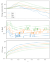Fig. 2. Energy conservation (top), the smallest resolved physical cell length (middle), and the runtime in CPU hours (bottom) for the main suite of simulations. Runs with a minimum refinement level of 8 are shown in solid lines, and 7 in dotted lines.

We find that N_min = 300, the mass enclosed by an approximately 7 × 7 × 7 cube, provides a reasonable estimate, as shown in Fig. 3. In this case M_min ≈ 10⁷ M_⊙ for l_init = 8, whereas at l_init = 7 the mass limit is M_min ≈ 10⁸ M_⊙. The profiles are largely the same except in the lowest mass bin, which is below M_min for l_init = 7. Additionally, the HMF is suppressed below M_min, hence halos with M₂₀₀ < M_min are discarded in the following analysis. It should be noted that the higher resolution yields slightly denser halos even for the masses that are most resolved, and that the HMF above M_min is not exactly identical at the two refinement levels, as one would expect. This indicates our simulations would benefit from further grid refinement, in particular the Rc1 run, which has the highest ratio of both M_min/M_cut and Δx_min/R_c. Unfortunately, the computational cost of further increasing the resolution was prohibitive, since at l_init = 8 the simulation used up to a hundred thousand CPU hours to reach z = 0.5, while an increase to the next refinement level l_init = 9 is expected to use a few million CPU hours.

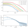Fig. 3. Binned SIBEC-DM halo profiles and the HMF for Rc = 1 kpc at z = 1.5, with minimum refinement level 7 (dotted) and 8 (solid). The HMF of CDM for the same box size and initial resolution is included in black. The halo mass limit Mmin are indicated by dots. The standard deviation from the binned halo profile mean for level 8, as well as the Poisson error in the HMF, are shown in shaded.

4. Results

In the cosmological simulations, the SIBEC-DM collapses and forms halos with a cored inner structure and a CDM-like envelope, which we find to be well-fitted by a cored NFW (NFWc) profile,

$$\begin{array}{c}\hfill {\delta }_{\mathrm{NFWc}}(r)={[{\delta }_{\mathrm{c}}^{-1}+{\delta }_{\mathrm{NFW}}^{-1}]}^{-1}.\end{array}$$(38)

The profile is given in terms of over-density $\delta =\rho /\overline{\rho }$, where δ_c is the central over-density, and δ_NFW is the NFW profile,

$$\begin{array}{c}\hfill {\delta }_{\mathrm{NFW}}(r)=\frac{{\delta }_{\mathrm{s}}}{\frac{r}{r_{\mathrm{s}}}{(1+\frac{r}{r_{\mathrm{s}}})}^2}·\end{array}$$(39)

We define the core radius r_c as where the density has dropped to 50% of its central value, δ(r_c) = 0.5δ(0). At hydrostatic equilibrium we would have r_c ≈ 0.6 R_c. A number of other cored profiles could also be used to fit the SIBEC-DM halos. In Li et al. (2020) several DM profiles were fitted to the Spitzer Photometry & Accurate Rotation Curves (SPARC) dataset of rotation curves of nearby galaxies (Lelli et al. 2016), such as the Burkert profile (Burkert 1995),

$$\begin{array}{c}\hfill {\delta }_{\mathrm{Burkert}}(r)=\frac{{\delta }_{\mathrm{c}}}{(1+\frac{r}{r_{\mathrm{s}}})[1+{\left(\frac{r}{r_{\mathrm{s}}}\right)}^2]},\end{array}$$(40)

the Einasto profile (Einasto 1965),

$$\begin{array}{c}\hfill {\delta }_{\mathrm{Einasto}}(r)={\delta }_{\mathrm{s}}exp\{-\frac{2}{{\alpha }_{ϵ}}[{\left(\frac{r}{r_{\mathrm{s}}}\right)}^{{\alpha }_{ϵ}}-1]\}\end{array}$$(41)

and the so-called Lucky13 profile (Li et al. 2020),

$$\begin{array}{c}\hfill {\delta }_{13}(r)=\frac{{\delta }_{\mathrm{c}}}{[1+{\left(\frac{r}{r_{\mathrm{s}}}\right)}^3]}·\end{array}$$(42)

These are fitted to the SIBEC-DM halos by minimizing the cost function

$$\begin{array}{c}\hfill {\chi }_{\nu }^2=\frac{1}{N_{\mathrm{d}}-N_{\mathrm{f}}}{\displaystyle \sum _{i=1}^{N_{\mathrm{d}}}}\frac{{[{\delta }_i-\delta (r_i)]}^2}{{\delta }_i^2},\end{array}$$(43)

with respect to the N_f free parameters of the density function δ(r), where N_d is the number of radial points δ_i from the simulation that we are fitting the density profile to. Each halo in the simulation gives a value for ${\chi }_{\nu }^2$, and the corresponding cumulative distribution function (CDF) for the set of these tells us what fraction of halos has ${\chi }_{\nu }^2$ smaller than a given value, and therefore how well the fitting function generally describes the halos. In Fig. 4 the CDF for the different types of profiles are shown, from which we find that the NFWc profile provides the best fit overall. Of the cored profiles used by Li et al. (2020) to fit the DM halos in the SPARC dataset, the Burkert and Einasto profiles are best suited and perform about the same, but as Burkert is the simpler of the two, we will use it in the following.

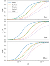Fig. 4. Cumulative distribution functions for different cored halo profiles from SIBEC-DM simulations with Rc = 1 kpc (upper), Rc = 3 kpc (middle), and Rc = 10 kpc (lower) at z = 0.5. This shows the fraction of the halos that has ${\chi }_v^2$ smaller than a given value, and therefore how well the fitting function generally describes the halos in our simulation.

Both NFWc and Burkert fitted to binned SIBEC-DM halos with R_c = 1 kpc at z = 0.5 are shown in Fig. 5. The two profiles yield slightly different results for the core radius. Burkert is a bit steeper than NFWc near the core, and therefore generally gives a core radius r_c of around half compared to NFWc (according to our definition δ(r_c) = 0.5δ(0)). The core density δ_c is also about twice as high for Burkert compared to NFWc. In the following we use the Burkert profile, even though the fit using NFWc is better, for two reasons; it is a simpler function, and we can readily compare the fitting parameters of the SIBEC-DM halos to observations, because the Burkert profile has previously been used for the DM component of nearby galaxies in the SPARC dataset (Li et al. 2020) and the dwarf spheroidal (dSph) satellites of the Milky Way (Salucci et al. 2012).

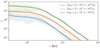Fig. 5. Mean (solid) and standard deviation (shaded) of binned SIBEC-DM halo profiles with Rc = 1 kpc at z = 0.5. The binned profiles are fitted to NFWc (dashed) and Burkert (dash-dotted). The fits of the NFW profile to the halo envelopes are also shown (dotted).

In order to investigate the general trends in the SIBEC-DM halos in our simulations, and compare these to observations, we introduce scaling functions for the core radius r_c, the central density δ_c, and the mass enclosed inside the core radius, M_c;

$$\begin{array}{cc}& r_{\mathrm{c}}(M_{200})=r_{\mathrm{c},10}{\left(\frac{M_{200}}{{10}^{10}{M}_{\odot }}\right)}^{\alpha },\hfill \end{array}$$(44)

$$\begin{array}{cc}& {\delta }_{\mathrm{c}}(M_{200})={\delta }_{\mathrm{c},10}{\left(\frac{M_{200}}{{10}^{10}{M}_{\odot }}\right)}^{\beta },\hfill \end{array}$$(45)

$$\begin{array}{cc}& M_{\mathrm{c}}(M_{200})=M_{\mathrm{c},10}{\left(\frac{M_{200}}{{10}^{10}{M}_{\odot }}\right)}^{\gamma }.\hfill \end{array}$$(46)

These are fitted using Theil-Sen regression (Theil 1950; Sen 1968). This method finds the slope m and the y-intercept b of the linear function y(x) = b + mx (which Eqs. (44)–(46) are in log-space) by first computing the median of slopes between all pairs of points (y_i, x_i), which gives m, and then finding the median of y_i − mx_i for all points, which gives b. This fitting procedure is robust against outliers, and provides a simple measure of the variation in m and b present in the data through, for example, the first and third quartiles of the pairwise slopes and individual y-intercepts. Tables listing the scaling parameters fitted using this procedure are included in Appendix A for several redshifts.

The properties of the Burkert profile fitted to SIBEC-DM halos are shown in Fig. 6 for R_c = 1 kpc, 3 kpc, and 10 kpc, along with the above scaling relations. The fit to the nearby galaxy rotation curves in the SPARC dataset (Li et al. 2020) and Milky Way dSphs (Salucci et al. 2012) are also included in Fig. 6.

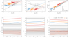Fig. 6. Core radii rc (left), core densities δc (middle), and core masses Mc (right) versus M200 for halos in cosmological simulations of SIBEC-DM with Rc = 1 kpc, 3 kpc, and 10 kpc, using the Burkert profile. The upper plots show the scatter of halos at z = 0.5, with the fitted scaling Eqs. (44)–(46) shown in dashed lines, compared to the SPARC dataset (Li et al. 2020) and Milky Way dSphs (Salucci et al. 2012). The lower plots show the fitted median (solid) and the first and third quartiles (shaded) at several redshifts using Theil-Sen regression. The results from SPARC and the dSphs are also shown. In the scatter plot for rc the core radii Rc are indicated in dotted colored lines.

While the halo catalogues from the simulation snapshots only span 2−3 orders in magnitude in mass and number 200−400 halos due to the limited volume of the simulated box, and the fitted parameters of the scaling functions show some time-dependence (the prefactors more so than the exponents), there are a number of interesting features to note. The halo core radii r_c are scattered near R_c, and the dependence of r_c on M₂₀₀ is nearly constant, largely as expected from hydrostatic considerations, although there is a slight positive trend, $r_{\mathrm{c}}\sim M_{200}^{\alpha }$ with α ≈ 0.05 − 0.1. Also, the SIBEC-DM cores are generally larger compared to what we find from Eq. (9). Both of these observations are consistent with the addition of thermal pressure in the halos centers, which is also slightly increasing for more massive halos, as seen in Fig. 7. In fact, the thermal-like energy due to the hidden dynamics on the de Broglie-scale dominates the central regions of the SIBEC-DM halos. This is illustrated in Fig. 8, where the self-interaction, thermal, and gravitational potential energy densities of a sample halo are shown. As structure forms, the SIBEC-DM fluid is heated as it is accreted onto the growing halos, the kinetic energy of the in-falling matter being converted into effective thermal energy. The result are halos with a thermal energy much larger than the interaction energy throughout the halo, even in the core where it dominates the overall dynamics. Additionally, the thermal energy is nearly isothermal. At the edge of the core the potential energy becomes larger than the internal energies, and the halo transitions to an NFW-like envelope.

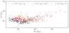Fig. 7. Ratio of average thermal and self-interaction energy, U and USI, inside the halo cores r < rc/2 in simulations with Rc = 3 kpc at z = 1.

We illustrate with the sample halo in Fig. 8, which is relatively isolated in the simulated box, that the SIBEC-DM halos in the simulations achieve approximate virial equilibrium. The virial 𝒱 satisfies, under the assumption of spherical symmetry (Dawoodbhoy et al. 2021),

$$\begin{array}{c}\hfill \mathcal{V}=2\mathcal{T}+\mathcal{W}+2\mathcal{U}+3{\mathcal{U}}_{\mathrm{SI}}+\mathcal{S}+{\mathcal{S}}_{\mathrm{SI}}=0,\end{array}$$(47)

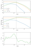Fig. 8. Top panel: self-interaction energy density USI, thermal energy density U, and gravitational potential energy density W of a sample halo with Rc = 1 kpc and M200 = 3 × 109 M⊙, relative to the interaction energy at the background level ${\overline{U}}_{\mathrm{SI}}$. The middle panel shows instead the specific energy, and the bottom panel the cumulative virial. The core radius rc and halo radius r200 are indicated with the inner and outer dotted vertical lines, respectively.

where the various terms are cumulative energy contributions and surface terms,

$$\begin{array}{cc}& \mathcal{T}=\frac{1}{2}\int v^2\mathrm{d}M-2\pi r^2(\rho r{v}^2+\frac{1}{2}{r}^2\frac{\partial (\rho v)}{\partial t}),\hfill \end{array}$$(48)

$$\begin{array}{cc}& \mathcal{W}=-{\displaystyle \int }\frac{\mathit{GM}}{r}\mathrm{d}M,\hfill \end{array}$$(49)

$$\begin{array}{cc}& \mathcal{U}={\displaystyle \int }\frac{U}{\rho }\mathrm{d}M,{\mathcal{U}}_{\mathrm{SI}}=\int \frac{U_{\mathrm{SI}}}{\rho }\mathrm{d}M,\hfill \end{array}$$(50)

$$\begin{array}{cc}& \mathcal{S}=-4\pi r^{3}P,{\mathcal{S}}_{\mathrm{SI}}=-4\pi r^3{P}_{\mathrm{SI}},\hfill \end{array}$$(51)

and 𝒰_tot = 𝒰 + 𝒰_SI.

Our 3D simulations confirm many of the features of SIBEC-DM halos that were reported in Dawoodbhoy et al. (2021), such as the transition from a cored interior to a CDM-like envelope near R_c, and the domination of the thermal energy over self-interaction energy outside the core due to shock heating. The only significant difference is the domination of thermal energy inside the cores of halos in 3D, whereas in 1D simulations the cores are not heated and are instead dominated by self-interactions. In fact, the halos from our simulations look more like the double-polytrope solutions of Dawoodbhoy et al. (2021) for SIBEC-DM with both the self-interaction pressure and an isothermal thermal pressure at hydrostatic equilibrium. Dawoodbhoy et al. (2021) anticipated that after collapse, relaxation, and finally virial equilibrium, the thermal profile should be nearly isothermal, with core radii set by the self-interaction pressure and thus on the order of R_c, which is what we find in our simulations.

We attribute the difference between our simulations and the ones in Dawoodbhoy et al. (2021) to the absence of mixing in spherical symmetry. In 1D, halos form by the accretion of spherically symmetric shells that are heated as they are slowed down, resulting in an accretion shock expanding outwards as shells collide, but do not cross. The cores themselves experience little heating as the fluid is decelerated smoothly by the self-interaction pressure and without a shock. In fully 3D simulations the halos form as clumps – not perfect shells – of matter merge, which perturb the halos and causes the outer shock heated layers to mix with the interior. We demonstrate this difference between symmetrical and asymmetrical collapse using 2D simulations; one in which an initial stationary over-density is centered in the simulated box and collapses symmetrically; and another with a second smaller over-density offset at x₂ that merges with the first in an asymmetrical manner. The initial density field in the two scenarios are ρ(x) = ρ₀ + ρ₀Δ₁e^{−(|x|/R₁)2}, and ρ(x) = ρ₀ + ρ₀Δ₁e^{−(|x|/R₁)2} + ρ₀Δ₂e^{−(|x − x₂|/R₂)2}, and we use a periodic box of size L = 40 kpc with R_c = 1 kpc, R₁ = 5 kpc, R₂ = 2 kpc, Δ₁ = Δ₂ = 99, |x₂| = 10 kpc, and ρ₀ = Ω_m0ρ_c0, with the initial ratio ζ = P/P_SI = 10⁻². The “symmetrical” simulation was run for 20 t_dyn, while the “asymmetrical” one was run for 200 t_dyn, to give it enough time to virialize, where $t_{\mathrm{dyn}}=1/\sqrt{2\pi G{\rho }_0{\mathrm{\Delta }}_1}$ is the dynamical timescale of the central over-density. The final distributions of U/U_SI are shown in Fig. 9. In the symmetrical case, the thermal energy is dominant everywhere except in the core, whereas in the asymmetrical case the merging with the second over-density results in a strong mixing of the fluid layers, causing shock-heated fluid in the region outside the core to penetrate into the core.

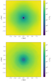Fig. 9. Final distributions of U/USI in 2D simulations with symmetrical (upper) and asymmetrical (lower) collapse, centered on the density peak. In the asymmetrical case, the second smaller over-density was initially located to the right. The minimum in the symmetrical case is around U/USI ≈ 2 × 10−2, while in the asymmetrical case its is U/USI ≈ 2.

In Fig. 10 the internal energies of SIBEC-DM with R_c = 1 kpc at z = 0.5 are shown, where the extended envelopes of high thermal energies compared to the interaction energy are clearly seen around the collapsed structures. In the same figure the density field is compared to standard CDM, which illustrates the smoothing of the DM density field, especially in the halo cores. The corresponding matter power spectrum is shown in Fig. 11 at several redshifts, as well as CDM with the same initial conditions, but without the cut-off, with

$$\begin{array}{c}\hfill {\mathrm{\Delta }}^2(k)=\frac{k^{3}P(k)}{2{\pi }^2},\end{array}$$(52)

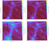Fig. 10. Projection plots of the DM density in cosmological simulations with L = 2 Mpc h−1 at z = 0.5 SIBEC-DM with Rc = 1 kpc (upper right) and CDM with the same initial conditions, but without a cut-off (upper left). The SIBCE-DM internal energies for the same snapshot showing the effective thermal energy U (lower left) and the self-interaction energy USI (lower right).

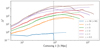Fig. 11. Matter power spectrum for cosmological simulations L = 2 Mpc h−1 at z = 0.5 for SIBEC-DM with R = 1 kpc (solid) and CDM (dashed). The comoving cut-off kcut is indicated with a dotted vertical line, and the spectrum at z = 50 is multiplied by 50 in the figure.

where

$$\begin{array}{c}\hfill {(2\pi )}^{3}P(k){\delta }^3(\mathit{k}-{\mathit{k}}^{\prime })=\widehat{\delta }(\mathit{k})\widehat{\delta }({\mathit{k}}^{\prime }),\end{array}$$(53)

and

$$\begin{array}{c}\hfill \widehat{\delta }(\mathit{k})={\displaystyle \int }{\mathrm{d}}^{3}x\delta (\mathit{x})e^{-i\mathit{k}·\mathit{x}},\end{array}$$(54)

with δ³ being the 3D Dirac delta function. At the largest scales the SIBEC-DM modes grow like CDM, while at smaller scales SIBEC-DM is suppressed compared to CDM due to the DM fluid pressure.

The simulations are insensitive to the initial ratio P/P_SI as long as it is much smaller than unity, as shown in Figs. 12 and 13. Below ζ = P/P_SI ≲ 0.1, there is little change in the final halos. As soon as structure begins to form, the thermal energy increases due to the conversion of kinetic energy to internal energy, hence, a small amount of initial thermal energy matters little. Nevertheless, despite the effective thermal energy dominating the DM-halo cores, it is the strength of the self-interaction that determines the characteristic size of the cores. This is because it is at the Jeans’ scale due to the self-interactions that the pressure forces begin opposing gravity, creating the shocks that cause the heating of the fluid.

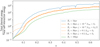Fig. 12. Evolution of the ratio of the total thermal energy and total self-interaction energy for the simulations run.

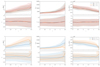Fig. 13. Scaling functions at several redshifts for the core radii rc (left), the core density δc (middle), and the core mass Mc (right) for SIBEC-DM halos with Rc = 3 kpc and different initial ζ = P/PSI (upper), and different initial power cut-offs (lower). The shaded areas give the first and third quartiles for the scaling parameters obtained from the Theil-Sen regression.

Another interesting feature is the dependence of δ_c on the halo mass. The Burkert profile fitted to observational data prefers a negative slope, meaning massive halos are less dense. In N-body simulations of CDM, considering instead the characteristic over-density δ_s of the halo in Eq. (39), such mass dependence arises, in very simple terms, because δ_s is proportional to the mean density at the time the halo forms, with low-mass halos generally collapsing at a higher redshift, when the universe was denser (Navarro et al. 1996). We might therefore expect processes that transform the CDM halo cusps into cores, for instance baryonic feedback, to produce core densities that inherit the same halo mass dependence (Ogiya et al. 2014). SIBEC-DM halos prefer instead a positive slope β ≈ 0.5 at z = 0.5, such that more massive halos are also denser. Furthermore, the SIBEC-DM halo core masses M_c scales approximately as $M_{\mathrm{c}}\sim M_{200}^{\gamma }$, with γ ≈ 0.75 at z = 0.5. The scaling of both M_c and δ_c can be qualitatively understood under the assumption of velocity dispersion tracing outside the core, meaning that the circular orbital velocity is nearly constant (Chavanis 2019a,b; Padilla et al. 2019; Dawoodbhoy et al. 2021),

$$\begin{array}{c}\hfill v_{\mathrm{c}}^2=\frac{G{M}_{\mathrm{c}}}{r_{\mathrm{c}}}\approx v_{200}^2=\frac{G{M}_{200}}{R_{200}},\end{array}$$(55)

which we indeed see to be approximately true in Fig. 8, since v² = −W/ρ. Inserting that r_c is constant, and $M_{200}\sim r_{200}^3$, gives

$$\begin{array}{c}\hfill M_{\mathrm{c}}\sim M_{200}^{2/3},\end{array}$$(56)

and

$$\begin{array}{c}\hfill {\delta }_{\mathrm{c}}\propto \frac{M_{\mathrm{c}}}{r_{\mathrm{c}}^3}\sim M_{200}^{2/3},\end{array}$$(57)

which are in the neighborhood of what is obtained in the simulations. We can improve this scaling argument by including a small mass dependence in $r_{\mathrm{c}}\sim M_{200}^{\alpha }$, which gives

$$\begin{array}{cc}& M_{\mathrm{c}}\sim M_{200}^{\frac{2}{3}+\alpha },\hfill \end{array}$$(58)

$$\begin{array}{cc}& {\delta }_{\mathrm{c}}\sim M_{200}^{\frac{2}{3}-2\alpha }.\hfill \end{array}$$(59)

Inserting α = 0.05 gives $M_{\mathrm{c}}\sim M_{200}^{0.72}$ and ${\delta }_{\mathrm{c}}\sim M_{200}^{0.57}$, while α = 0.1 gives $M_{\mathrm{c}}\sim M_{200}^{0.77}$ and ${\delta }_{\mathrm{c}}\sim M_{200}^{0.47}$. For comparison, independent FDM simulations, using the full NLSE or the Madelung equations, find varying exponents, with $M_{\mathrm{c}}\sim M_{200}^{1/3}$ (Schive et al. 2014a,b; Veltmaat et al. 2018), $M_{\mathrm{c}}\sim M_{200}^{5/9}$ (Mocz et al. 2017; Mina et al. 2022), or $M_{\mathrm{c}}\sim M_{200}^{0.6}$ (Nori & Baldi 2021), all of which are less steep than what we find for SIBEC-DM. Furthermore, as expected from hydrostatic equilibrium, the size of FDM halo cores have been found to be decreasing with the virial mass (Chan et al. 2022), as opposed to slightly increasing for SIBEC-DM.

Generally, we find the trends in r_c, δ_c, and M_c for the values of R_c and initial conditions tested in this paper to be in conflict with the SPARC dataset and Milky Way dSphs, although their slopes are in less tension with observations compared to FDM. The trends are mostly insensitive to the initial ratio P/P_SI ≪ 1, but they are dependent on the cut-off scale in the initial matter power spectrum (when it is not scaled along with R_c to match the Jeans’ length), as shown in Fig. 13. By moving the initial cut-off to larger scales, such that there is less initial power at small scales, the scaling exponents shift towards those inferred from the SPARC dataset and the Milky Way dSphs. On the flip-side, the prefactors shift away from the observations. For example, the total ratio P/P_SI increases as k_cut is lowered, meaning there is more thermal pressure, causing halos to have larger cores and lower central densities. However, as we saw in Fig. 6, decreasing the interaction strength, or equivalently, the core radius R_c, hardly affects the scaling exponents, but moves the prefactors in the desired direction. Based on this observation, one could imagine that a sufficiently small R_c and strong cut-off might create a population of halos that alleviates to some degree the current tension with the observed trends. According to Eqs. (58) and (59), a stronger mass dependence in the core radius $r_{\mathrm{c}}\sim M_{200}^{\alpha }$ will bring the SIBEC trends towards the observed ones, and can come about by having a larger thermal Jeans’ length for massive halos, such that more massive halos have a larger ratio of thermal energy to self-interaction energy, U/U_SI, due to increased heating, as observed in our simulations.

However, a good deal of caution is called for in making such a statement. For instance, the range of halo masses represented in the simulations is rather small, and baryonic physics are not included at all, but are known to affect the distribution of DM in halos. Furthermore, the scaling function parameters have some time-dependence, primarily the prefactors, and our simulations were only run until z = 0.5, whereas the observed galaxies and dSphs are at z ≈ 0. This is particularly true for the Rc3-b run with k_cut = k_J/2, which has about a fourth of the halos compared to k_cut = k_J, and is therefore more sensitive to disruptions in parts of the simulated halo population due to events such as mergers. We see this in Fig. 13 at z = 0.5, where the scaling parameters suddenly change, and the first and third quartile-region becomes very large, signaling that the scaling relations generally do not provide a good fit to the halo population at that point. Finally, but not least, the SIBEC-DM parameter space and initial conditions used in our simulations are not appropriate for a realistic realization of scalar field DM with self-interactions as given by the Lagrangian in Eq. (1), for which R_c ≳ 1 kpc are ruled out and the suppression in the initial power spectrum is much stronger (Shapiro et al. 2021; Hartman et al. 2022).

5. Conclusion

In this paper, a hydrodynamic approximation of the NLSE that includes the de Broglie-scale dynamics as an effective thermal energy was used to simulate the formation of structure of SIBEC-DM in a fully 3D cosmological setting. The advantage of such an approach is that the dynamics on the de Broglie-scale need not be resolved on the numerical grid, making the task of simulating SIBEC-DM simpler and computationally tractable. This is of particular importance when the de Broglie wavelength is much smaller than the self-interaction Jeans’ scale that we are interested in. On the other hand, this approach introduces an additional equation for the effective thermal energy that must be evolved through time, information about the underlying wavefunction is lost, and some simplifying assumptions were made, such as the skewlessness of the phase space distribution function.

Our simulations reproduce many of the features reported in Dawoodbhoy et al. (2021). The SIBEC-DM halos have cores with radii of order R_c, which is only weakly dependent on the halo mass. Outside the cores the halos transition to a CDM-like profile, which in our 3D simulations is the NFW profile. The SIBEC-DM halos are therefore generally well-described by a cored NFW-profile such as NFWc, Eq. (38), or the Burkert profile, Eq. (40). Despite the self-interactions determining the scale of the cores, the effective thermal energy ends up dominating over the self-interactions throughout the halos due to significant heating during collapse, even in the central regions. This is in contrast to the 1D simulations of Dawoodbhoy et al. (2021), who found the SIBEC-DM halo cores to not experience much heating, and the thermal energy to fall sharply below the self-interaction energy inside the core radius. However, Dawoodbhoy et al. (2021) anticipated that after collapse and relaxation, the SIBEC-DM halos should be largely isothermal with the central thermal energy on the order of the self-interaction energy. Spherically symmetric 1D simulations do not include the mixing of fluid layers that allows for such heating of the core, while in 3D, matter collapses onto the halos in clumps rather than shells, causing the outer shock-heated layers to be mixed with the central fluid, resulting in an isothermal profile. Our simulations therefore confirm this anticipated result of Dawoodbhoy et al. (2021).

Scaling relations for the core radii r_c, core densities δ_c, and core masses M_c as functions of the total halo mass M₂₀₀ were fitted to the simulated halo populations, which largely agree with hydrostatic considerations of the halo cores where r_c is nearly constant, as well as velocity dispersion tracing in the halo envelope, $v_{\text{c}}^2\approx v_{200}^2$. However, these trends do not agree with those obtained by fitting the Burkert profile to nearby galaxies in the SPARC dataset and the classical Milky Way dSphs. This poses an issue for SIBEC-DM with R_c ≳ 1 kpc and a largely CDM-like matter power spectrum at late times (Harko 2011; Harko & Mocanu 2012; Velten & Wamba 2012; Freitas & Gonçalves 2013; Bettoni et al. 2014; de Freitas & Velten 2015; Hartman et al. 2022), as was used in our simulations, although these scenarios are not well-motivated. For SIBEC-DM given by the field Lagrangian in Eq. (1), the self-interaction is constrained to R_c < 1 kpc, otherwise an early radiation-like period and a large comoving Jeans’ length washes out too much structure to be consistent with observations (Shapiro et al. 2021; Hartman et al. 2022). In fact, Shapiro et al. (2021) found by using constraints on FDM as a proxy for SIBEC-DM, and matching their transfer function cut-offs and HMFs, that the SIBEC-DM self-interaction should be as low as R_c ∼ 10 pc to not be in conflict with observations. We were unable to probe SIBEC-DM with initial conditions and parameters consistent with the Lagrangian in Eq. (1), since the large gap between the halo cores and the cut-off scale requires both a large simulation box and very high spatial resolution. It should be noted that our SIBEC-DM-only simulations do provide a better agreement with the slopes in observed scaling relations than FDM. In particular, FDM simulations generally find $M_{\mathrm{c}}\sim M_{200}^{\gamma }$ with 1/3 < γ < 0.6, while we find γ ≈ 0.75, which is closer to the observed γ ≈ 1.1. Additionally, FDM halos have core radii that generally decrease with the halo mass, while we find a slightly increasing trend due to larger halos experiencing more thermal heating, although not as steep as in the SPARC dataset and the Milky Way dSphs.

The main results of the present work is summarized as follows:

• Using a hydrodynamic approximation and fully 3D cosmological simulations, SIBEC-DM halos are found to have NFW-like envelopes with central core radii of order R_c. This confirms the results reported in Shapiro et al. (2021), based on 1D spherically symmetric simulations in the same hydrodynamic approximation, when the initial perturbation is chosen to yield an infall rate that matches the mass assembly history of 3D N-body simulations of CDM. The density profiles are therefore well-fitted by cored NFW profiles such as NFWc, Eq. (38), and the Burkert profile, Eq. (40).

• The SIBEC-DM core radii are only weakly dependent on the halo mass, largely as expected from hydrostatic equilibrium. The slight increase is due to larger halos generally experiencing more heating, and hence an increase in their thermal Jeans’ length.

• Despite the self-interaction energy initially dominating the internal energy and fluid pressure of the SIBEC-DM, as well as determining the general scale of the SIBEC-DM cores, the effective thermal energy ends up dominating throughout the halo. This result is insensitive to the initial ratio of the thermal energy relative to the self-interaction energy, as long as it is small, since the final thermal energy comes from heating as SIBEC-DM collapses and forms structure. Below ζ = P/P_SI ≲ 0.1, there are hardly any changes in the final halos.

• The SIBEC-DM halo core densities δ_c and core masses M_c are found to scale with the virial mass M₂₀₀ as ${\delta }_{\mathrm{c}}\sim M_{200}^{0.5}$ and $M_{\mathrm{c}}\sim M_{200}^{0.75}$. This result is insensitive to changes in R_c that is matched by a corresponding change in the cut-off scale, k_cut ∼ 1/R_c. Velocity tracing in the halo envelope and a nearly constant core radius predict these relations to be ${\delta }_{\mathrm{c}}\sim M_{\mathrm{c}}\sim M_{200}^{2/3}$. Including a small mass dependence in r_c improves the agreement with the simulations, $r_{\mathrm{c}}\sim M_{200}^{0.05}$, gives $M_{\mathrm{c}}\sim M_{200}^{0.72}$ and ${\delta }_{\mathrm{c}}\sim M_{200}^{0.57}$.

• The scaling relations for r_c(M₂₀₀), δ_c(M₂₀₀), and M_c(M₂₀₀), Eqs. (44)–(46), assuming the Burkert profile for the SIBEC-DM halos, generally do not agree with trends of the classical Milky Way dSphs and nearby galaxies in the SPARC dataset for the SIBEC-DM parameters tested in this work. Nevertheless, the slopes of the scaling relations in our SIBEC-DM-only simulation are in better agreement with observations compared to FDM-only simulations.

In future work, larger high-resolution simulations should be carried out to further investigate SIBEC-DM, as our current simulations have a limited box size and halo population. This is particularly relevant for probing SIBEC-DM with realistic initial conditions and self-interactions that are consistent with the HMF (Shapiro et al. 2021) and large-scale observables (Hartman et al. 2022). It will be important to test the validity and accuracy of the smoothing procedure and the resulting hydrodynamic approximation used in this work, especially if it continues to be used to test SIBEC-DM models. Dawoodbhoy et al. (2021) showed analytically for a few idealized 1D cases that smoothing the exact solutions of the NLSE gives the same large-scale fluid properties, such as pressure and density, as the smoothed phase space distribution function. These tests should be extended to more complicated scenarios, such as self-gravitation and the formation of shock fronts, to check, for instance, if the heating of the effective thermal energy is accurately captured by the hydrodynamic approximation, or if the skewlessness of ℱ is a valid assumption, both inside virialized halos and during the in-fall and collapse. In particular, the assumption of skewlessness should be tested in mergers, since the merging SIBEC-DM halos can have large plane-wave velocity dispersions, which would have significant implications for the merger event, although this will require using large and costly numerical simulations.

Acknowledgments

We thank the Research Council of Norway for their support, and the anonymous referee for their helpful comments and suggestions. We are also grateful to Matteo Nori and Marco Baldi for our discussions on simulations of ultra-light DM, and to Taha Dawoodbhoy and Paul R. Shapiro for their feedback on this work. Computations were performed on resources provided by UNINETT Sigma2 – the National Infrastructure for High Performance Computing and Data Storage in Norway.

References

Appendix A: Fitted scaling relation parameters

The fitted parameters for the scaling relations of r_c(M₂₀₀), δ_c(M₂₀₀), and M_c(M₂₀₀), Eqs. (44), (45), and (46), are shown in Tables A.1, A.2, and A.3. These values correspond to the fits shown in Figs. 6 and 13 obtained using Theil-Sen regression, including the results for the SPARC dataset (Li et al. 2020) and the Milky Way dSphs (Salucci et al. 2012).

All Tables

All Figures

Fig. 1. Self-interaction energy density USI, thermal energy density U, and gravitational potential energy density W of the spherically symmetric test halo with Rc = 1 kpc, relative to the interaction energy of the initial background ${\overline{U}}_{\mathrm{SI}}$. The result of the simulation with refinement levels 8 to 12 are shown in solid, while 7 to 11 is shown in dotted. The 3D simulation reproduces the 1D results of Ahn & Shapiro (2005) and Dawoodbhoy et al. (2021), in particular the large thermal energy in the wake of the accretion shock, its sharp decrease to below the self-interaction energy inside the core, and the fit USI ∝ ρ2 ∝ r−24/7 in the envelope.

In the text

	Fig. 2. Energy conservation (top), the smallest resolved physical cell length (middle), and the runtime in CPU hours (bottom) for the main suite of simulations. Runs with a minimum refinement level of 8 are shown in solid lines, and 7 in dotted lines.
In the text

	Fig. 3. Binned SIBEC-DM halo profiles and the HMF for Rc = 1 kpc at z = 1.5, with minimum refinement level 7 (dotted) and 8 (solid). The HMF of CDM for the same box size and initial resolution is included in black. The halo mass limit Mmin are indicated by dots. The standard deviation from the binned halo profile mean for level 8, as well as the Poisson error in the HMF, are shown in shaded.
In the text

	Fig. 4. Cumulative distribution functions for different cored halo profiles from SIBEC-DM simulations with Rc = 1 kpc (upper), Rc = 3 kpc (middle), and Rc = 10 kpc (lower) at z = 0.5. This shows the fraction of the halos that has ${\chi }_v^2$ smaller than a given value, and therefore how well the fitting function generally describes the halos in our simulation.
In the text

	Fig. 5. Mean (solid) and standard deviation (shaded) of binned SIBEC-DM halo profiles with Rc = 1 kpc at z = 0.5. The binned profiles are fitted to NFWc (dashed) and Burkert (dash-dotted). The fits of the NFW profile to the halo envelopes are also shown (dotted).
In the text

Fig. 6. Core radii rc (left), core densities δc (middle), and core masses Mc (right) versus M200 for halos in cosmological simulations of SIBEC-DM with Rc = 1 kpc, 3 kpc, and 10 kpc, using the Burkert profile. The upper plots show the scatter of halos at z = 0.5, with the fitted scaling Eqs. (44)–(46) shown in dashed lines, compared to the SPARC dataset (Li et al. 2020) and Milky Way dSphs (Salucci et al. 2012). The lower plots show the fitted median (solid) and the first and third quartiles (shaded) at several redshifts using Theil-Sen regression. The results from SPARC and the dSphs are also shown. In the scatter plot for rc the core radii Rc are indicated in dotted colored lines.

In the text

	Fig. 7. Ratio of average thermal and self-interaction energy, U and USI, inside the halo cores r < rc/2 in simulations with Rc = 3 kpc at z = 1.
In the text

Fig. 8. Top panel: self-interaction energy density USI, thermal energy density U, and gravitational potential energy density W of a sample halo with Rc = 1 kpc and M200 = 3 × 109 M⊙, relative to the interaction energy at the background level ${\overline{U}}_{\mathrm{SI}}$. The middle panel shows instead the specific energy, and the bottom panel the cumulative virial. The core radius rc and halo radius r200 are indicated with the inner and outer dotted vertical lines, respectively.

In the text

	Fig. 9. Final distributions of U/USI in 2D simulations with symmetrical (upper) and asymmetrical (lower) collapse, centered on the density peak. In the asymmetrical case, the second smaller over-density was initially located to the right. The minimum in the symmetrical case is around U/USI ≈ 2 × 10−2, while in the asymmetrical case its is U/USI ≈ 2.
In the text

	Fig. 10. Projection plots of the DM density in cosmological simulations with L = 2 Mpc h−1 at z = 0.5 SIBEC-DM with Rc = 1 kpc (upper right) and CDM with the same initial conditions, but without a cut-off (upper left). The SIBCE-DM internal energies for the same snapshot showing the effective thermal energy U (lower left) and the self-interaction energy USI (lower right).
In the text

	Fig. 11. Matter power spectrum for cosmological simulations L = 2 Mpc h−1 at z = 0.5 for SIBEC-DM with R = 1 kpc (solid) and CDM (dashed). The comoving cut-off kcut is indicated with a dotted vertical line, and the spectrum at z = 50 is multiplied by 50 in the figure.
In the text

	Fig. 12. Evolution of the ratio of the total thermal energy and total self-interaction energy for the simulations run.
In the text

	Fig. 13. Scaling functions at several redshifts for the core radii rc (left), the core density δc (middle), and the core mass Mc (right) for SIBEC-DM halos with Rc = 3 kpc and different initial ζ = P/PSI (upper), and different initial power cut-offs (lower). The shaded areas give the first and third quartiles for the scaling parameters obtained from the Theil-Sen regression.
In the text

References

- Ahn, K., & Shapiro, P. R. 2005, MNRAS, 363, 1092 [NASA ADS] [CrossRef] [Google Scholar]
- Arbey, A., Lesgourgues, J., & Salati, P. 2002, Phys. Rev. D, 65, 083514 [NASA ADS] [CrossRef] [Google Scholar]
- Arbey, A., Lesgourgues, J., & Salati, P. 2003, Phys. Rev. D, 68, 023511 [NASA ADS] [CrossRef] [Google Scholar]
- Berezhiani, L., & Khoury, J. 2015, Phys. Rev. D, 92, 103510 [Google Scholar]
- Berezhiani, L., Elder, B., & Khoury, J. 2019, JCAP, 2019, 074 [Google Scholar]
- Bettoni, D., Colombo, M., & Liberati, S. 2014, JCAP, 2014, 004 [CrossRef] [Google Scholar]
- Bullock, J. S., & Boylan-Kolchin, M. 2017, ARA&A, 55, 343 [Google Scholar]
- Burkert, A. 1995, ApJ, 447, L25 [NASA ADS] [Google Scholar]
- Böhmer, C. G., & Harko, T. 2007, JCAP, 2007, 025 [CrossRef] [Google Scholar]
- Chan, H. Y. J., Ferreira, E. G. M., May, S., Hayashi, K., & Chiba, M. 2022, MNRAS, 511, 943 [NASA ADS] [CrossRef] [Google Scholar]
- Chavanis, P.-H. 2011, Phys. Rev. D, 84, 043531 [NASA ADS] [CrossRef] [Google Scholar]
- Chavanis, P.-H. 2019a, Phys. Rev. D, 100, 123506 [NASA ADS] [CrossRef] [Google Scholar]
- Chavanis, P.-H. 2019b, Phys. Rev. D, 100, 083022 [NASA ADS] [CrossRef] [Google Scholar]
- Chavanis, P.-H., & Delfini, L. 2011, Phys. Rev. D, 84, 043532 [NASA ADS] [CrossRef] [Google Scholar]
- Crăciun, M., & Harko, T. 2020, Eur. Phys. J. C, 80, 735 [CrossRef] [Google Scholar]
- Cyburt, R. H., Fields, B. D., Olive, K. A., & Yeh, T.-H. 2016, Rev. Mod. Phys., 88, 015004 [NASA ADS] [CrossRef] [Google Scholar]
- Davis, M., Efstathiou, G., Frenk, C. S., & White, S. D. M. 1985, ApJ, 292, 371 [Google Scholar]
- Dawoodbhoy, T., Shapiro, P. R., & Rindler-Daller, T. 2021, MNRAS, 506, 2418 [NASA ADS] [CrossRef] [Google Scholar]
- de Freitas, R. C., & Velten, H. 2015, Eur. Phys. J. C, 75, 597 [NASA ADS] [CrossRef] [Google Scholar]
- Del Popolo, A., & Le Delliou, M. 2017, Galaxies, 5, 17 [Google Scholar]
- Dine, M., & Fischler, W. 1983, Phys. Lett. B, 120, 137 [NASA ADS] [CrossRef] [Google Scholar]
- Einasto, J. 1965, Trudy Astrofizicheskogo Instituta Alma-Ata, 5, 87 [NASA ADS] [Google Scholar]
- Ferreira, E. G. M. 2021, A&ARv, 29, 1 [NASA ADS] [CrossRef] [Google Scholar]
- Ferreira, E. G. M., Franzmann, G., Khoury, J., & Brandenberger, R. 2019, JCAP, 2019, 027 [CrossRef] [Google Scholar]
- Freitas, R. C., & Gonçalves, S. V. B. 2013, JCAP, 2013, 049 [CrossRef] [Google Scholar]
- Gill, S. P. D., Knebe, A., & Gibson, B. K. 2004, MNRAS, 351, 399 [Google Scholar]
- Goodman, J. 2000, New Astron., 5, 103 [NASA ADS] [CrossRef] [Google Scholar]
- Hahn, O., & Abel, T. 2011, MNRAS, 415, 2101 [Google Scholar]
- Harko, T. 2011, Phys. Rev. D, 83, 123515 [NASA ADS] [CrossRef] [Google Scholar]
- Harko, T., & Mocanu, G. 2012, Phys. Rev. D, 85, 084012 [Google Scholar]
- Hartman, S. T. H., Winther, H. A., & Mota, D. F. 2022, JCAP, 2022, 005 [CrossRef] [Google Scholar]
- Hu, W., Barkana, R., & Gruzinov, A. 2000, Phys. Rev. Lett., 85, 1158 [NASA ADS] [CrossRef] [Google Scholar]
- Huang, K. 1987, Statistical Mechanics, 2nd edn. (John Wiley& Sons) [Google Scholar]
- Hui, L., Ostriker, J. P., Tremaine, S., & Witten, E. 2017, Phys. Rev. D, 95, 043541 [NASA ADS] [CrossRef] [Google Scholar]
- Husimi, K. 1940, Proc. Physico-Math. Soc. Jpn., 22, 264 [Google Scholar]
- Khoury, J. 2016, Phys. Rev. D, 93, 103533 [Google Scholar]
- Knollmann, S. R., & Knebe, A. 2009, ApJS, 182, 608 [Google Scholar]
- Lancaster, L., Giovanetti, C., Mocz, P., et al. 2020, JCAP, 2020, 001 [Google Scholar]
- Lee, J.-W., & Koh, I.-G. 1996, Phys. Rev. D, 53, 2236 [Google Scholar]
- Lelli, F., McGaugh, S. S., & Schombert, J. M. 2016, AJ, 152, 157 [Google Scholar]
- Li, B., Rindler-Daller, T., & Shapiro, P. R. 2014, Phys. Rev. D, 89, 083536 [NASA ADS] [CrossRef] [Google Scholar]
- Li, P., Lelli, F., McGaugh, S., & Schombert, J. 2020, ApJS, 247, 31 [Google Scholar]
- Madelung, E. 1926, Naturwissenschaften, 14, 1004 [Google Scholar]
- Marsh, D. J. E. 2016, Phys. Rep., 643, 1 [NASA ADS] [CrossRef] [Google Scholar]
- Martel, H., & Shapiro, P. R. 1998, MNRAS, 297, 467 [Google Scholar]
- Matos, T., & Arturo Ureña-López, L. 2001, Phys. Rev. D, 63, 063506 [NASA ADS] [CrossRef] [Google Scholar]
- Matos, T., Guzmán, F. S., & Ureña-López, L. A. 2000, Class. Quant. Grav., 17, 1707 [NASA ADS] [CrossRef] [Google Scholar]
- May, S., & Springel, V. 2021, MNRAS, 506, 2603 [NASA ADS] [CrossRef] [Google Scholar]
- Membrado, M., Pacheco, A. F., & Sañudo, J. 1989, Phys. Rev. A, 39, 4207 [NASA ADS] [CrossRef] [Google Scholar]
- Mina, M., Mota, D. F., & Winther, H. A. 2020, A&A, 641, A107 [EDP Sciences] [Google Scholar]
- Mina, M., Mota, D. F., & Winther, H. A. 2022, A&A, 662, A29 [NASA ADS] [CrossRef] [EDP Sciences] [Google Scholar]
- Mocz, P., Vogelsberger, M., Robles, V. H., et al. 2017, MNRAS, 471, 4559 [Google Scholar]
- Mocz, P., Lancaster, L., Fialkov, A., Becerra, F., & Chavanis, P.-H. 2018, Phys. Rev. D, 97, 083519 [NASA ADS] [CrossRef] [Google Scholar]
- Navarro, J. F., Frenk, C. S., & White, S. D. M. 1996, ApJ, 462, 563 [Google Scholar]
- Navarro, J. F., Frenk, C. S., & White, S. D. M. 1997, ApJ, 490, 493 [Google Scholar]
- Nori, M., & Baldi, M. 2018, MNRAS, 478, 3935 [Google Scholar]
- Nori, M., & Baldi, M. 2021, MNRAS, 501, 1539 [Google Scholar]
- Ogiya, G., Mori, M., Ishiyama, T., & Burkert, A. 2014, MNRAS, 440, L71 [NASA ADS] [CrossRef] [Google Scholar]
- Padilla, L. E., Rindler-Daller, T., Shapiro, P. R., Matos, T., & Vázquez, J. A. 2019, Phys. Rev. D, 103, 063012 [Google Scholar]
- Peebles, P. J. E. 2000, ApJ, 534, L127 [NASA ADS] [CrossRef] [Google Scholar]
- Percival, W. J., Baugh, C. M., Bland-Hawthorn, J., et al. 2001, MNRAS, 327, 1297 [Google Scholar]
- Pitaevskii, L. P., & Stringari, S. 2016, Bose-Einstein Condensation and Superfluidity (Oxford: Oxford University Press) [Google Scholar]
- Planck Collaboration XIII. 2016, A&A, 594, A13 [NASA ADS] [CrossRef] [EDP Sciences] [Google Scholar]
- Preskill, J., Wise, M. B., & Wilczek, F. 1983, Phys. Lett. B, 120, 127 [NASA ADS] [CrossRef] [Google Scholar]
- Riess, A. G., Macri, L. M., Hoffmann, S. L., et al. 2016, ApJ, 826, 56 [Google Scholar]
- Rindler-Daller, T., & Shapiro, P. R. 2012, MNRAS, 422, 135 [NASA ADS] [CrossRef] [Google Scholar]
- Rindler-Daller, T., & Shapiro, P. R. 2014, Mod. Phys. Lett. A, 29, 1430002 [NASA ADS] [CrossRef] [Google Scholar]
- Robles, V. H., Bullock, J. S., & Boylan-Kolchin, M. 2019, MNRAS, 483, 289 [NASA ADS] [CrossRef] [Google Scholar]
- Rogers, K. K., & Peiris, H. V. 2021, Phys. Rev. Lett., 126, 071302 [NASA ADS] [CrossRef] [Google Scholar]
- Salucci, P., Wilkinson, M. I., Walker, M. G., et al. 2012, MNRAS, 420, 2034 [NASA ADS] [CrossRef] [Google Scholar]
- Schive, H.-Y., Chiueh, T., & Broadhurst, T. 2014a, Nat. Phys., 10, 496 [NASA ADS] [CrossRef] [Google Scholar]
- Schive, H.-Y., Liao, M.-H., Woo, T.-P., et al. 2014b, Phys. Rev. Lett., 113, 261302 [NASA ADS] [CrossRef] [Google Scholar]
- Schwabe, B., Niemeyer, J. C., & Engels, J. F. 2016, Phys. Rev. D, 94, 043513 [Google Scholar]
- Sen, P. K. 1968, J. Am. Stat. Assoc., 63, 1379 [CrossRef] [Google Scholar]
- Shapiro, P. R., Dawoodbhoy, T., & Rindler-Daller, T. 2021, MNRAS, 509, 145 [NASA ADS] [CrossRef] [Google Scholar]
- Skodje, R. T., Rohrs, H. W., & VanBuskirk, J. 1989, Phys. Rev. A, 40, 2894 [NASA ADS] [CrossRef] [Google Scholar]
- Tegmark, M., Blanton, M. R., Strauss, M. A., et al. 2004, ApJ, 606, 702 [Google Scholar]
- Teyssier, R. 2002, A&A, 385, 337 [CrossRef] [EDP Sciences] [Google Scholar]
- Theil, H. 1950, Nederl. Akad. Wetensch. Proc., 53, 386 [Google Scholar]
- Toro, E. 2006, Appl. Numer. Math., 56, 1464 [Google Scholar]
- Trujillo-Gomez, S., Klypin, A., Primack, J., & Romanowsky, A. J. 2011, ApJ, 742, 16 [Google Scholar]
- Turk, M. J., Smith, B. D., Oishi, J. S., et al. 2010, ApJS, 192, 9 [Google Scholar]
- Velten, H., & Wamba, E. 2012, Phys. Lett. B, 709, 1 [NASA ADS] [CrossRef] [Google Scholar]
- Veltmaat, J., Niemeyer, J. C., & Schwabe, B. 2018, Phys. Rev. D, 98, 043509 [NASA ADS] [CrossRef] [Google Scholar]
- Vogelsberger, M., Genel, S., Springel, V., et al. 2014, Nature, 509, 177 [Google Scholar]
- Weinberg, D. H., Bullock, J. S., Governato, F., Naray, R. K. D., & Peter, A. H. G. 2015, Proc. Natl. Acad. Sci., 112, 12249 [Google Scholar]
- Widrow, L. M., & Kaiser, N. 1993, ApJ, 416, L71 [NASA ADS] [CrossRef] [Google Scholar]
- Zhang, X., Chan, M. H., Harko, T., Liang, S.-D., & Leung, C. S. 2018, Eur. Phys. J. C, 78, 346 [NASA ADS] [CrossRef] [Google Scholar]