| Issue |
A&A
Volume 696, April 2025
|
|
|---|---|---|
| Article Number | A25 | |
| Number of page(s) | 13 | |
| Section | Astrophysical processes | |
| DOI | https://doi.org/10.1051/0004-6361/202553662 | |
| Published online | 28 March 2025 | |
Tension of the toroidal magnetic field in reconnection plasmoids and relativistic jets
Nicolaus Copernicus Astronomical Center, Polish Academy of Sciences, Bartycka 18, 00-716 Warsaw, Poland
⋆ Corresponding author; This email address is being protected from spambots. You need JavaScript enabled to view it.
Received:
2
January
2025
Accepted:
18
February
2025
Abstract
The toroidal magnetic field is a key ingredient of relativistic jets launched by certain accreting astrophysical black holes, and of plasmoids emerging from the tearing instability during magnetic reconnection, which is a candidate dissipation mechanism in jets. Tension of the toroidal field is an anisotropic force that can compress local energy and momentum densities. We investigate this effect in plasmoids produced during relativistic reconnection initiated from a Harris layer by means of kinetic particle-in-cell numerical simulations, varying the system size (including 3D cases), magnetisation, or guide field. We find that: (1) plasmoid cores are dominated by plasma energy density for guide fields up to Bz ∼ B0; (2) relaxed ‘monster’ plasmoids compress plasma energy density only modestly (by a factor of ∼3 above the initial level for the drifting particle population); (3) energy density compressions by factors ≳10 are achieved during plasmoid mergers, especially with the emergence of secondary plasmoids. This kinetic-scale effect can be combined with a global focusing of the jet Poynting flux along the quasi-cylindrical bunched spine (a proposed jet layer adjacent to the cylindrical core) due to poloidal line bunching (a prolonged effect of tension in the jet toroidal field) to enhance the luminosity of rapid radiation flares from blazars. The case of M87 as a misaligned blazar is discussed.
Key words: magnetic fields / magnetic reconnection / relativistic processes / methods: numerical / galaxies: active / galaxies: jets
© The Authors 2025
 Open Access article, published by EDP Sciences, under the terms of the Creative Commons Attribution License (https://creativecommons.org/licenses/by/4.0), which permits unrestricted use, distribution, and reproduction in any medium, provided the original work is properly cited.
This article is published in open access under the Subscribe to Open model. This email address is being protected from spambots. You need JavaScript enabled to view it. to support open access publication.
1. Introduction
Extremely luminous, highly variable, non-thermal, high-energy cosmic sources of radiation are often interpreted as originating from powerful collimated outflows known as relativistic jets (Madejski & Sikora 2016; Blandford et al. 2019). In many supermassive active galactic nuclei (AGNs), narrow jets and their relativistic motions can be observed directly (e.g. Jorstad et al. 2001; Lister et al. 2016). In the subclass of blazars, a small viewing angle allows for a huge (∼105) relativistic boost of non-thermal radiation produced by particles accelerated during dissipative processes in the approaching jet (Urry & Padovani 1995). The most luminous blazars, belonging to the subclass of flat-spectrum radio quasars (FSRQs), produce giga-electronvolt γ-ray flares with apparent luminosities of Lfl, FSRQ ∼ 1050 erg s−1 and variability timescales of tfl, FSRQ ∼ 10 min (e.g. Abdo et al. 2011; Ackermann et al. 2016; Shukla & Mannheim 2020)1. Another subclass of blazars, high-energy peaked BL Lac objects (HBLs), produce tera-electronvolt γ-ray flares with apparent luminosities of Lfl, HBL ∼ 1047 erg s−1 and variability timescales of tfl, HBL ∼ 3 min (Aharonian et al. 2007). Even after accounting for the relativistic boost, the energetic requirements for the blazar zones can be very demanding in terms of local energy density and radiative efficiency (e.g. Nalewajko et al. 2012; Ackermann et al. 2016; Appendix A).
The toroidal magnetic field is an essential ingredient of relativistic jets launched by magnetised accretion onto spinning black holes ((BHs); e.g. Begelman et al. 1984; Davis & Tchekhovskoy 2020). It is the main carrier of electromagnetic momentum (Poynting) flux (the initial form of jet power) (Blandford 1976). Its pressure acting along the velocity streamlines is the primary agent of acceleration to relativistic speeds (e.g. Camenzind 1989; Komissarov et al. 2007). In jet regions that expand laterally, the toroidal field decreases slower than the poloidal field, likely becoming the dominant component at distances of ∼0.1 − 1 pc typically inferred for emission of blazar flares (Nalewajko et al. 2014).
Toroidal magnetic field is also an essential ingredient of plasmoids (flux ropes) produced during large-scale magnetic reconnection due to the tearing instability of thin current sheets (Furth et al. 1963; Loureiro et al. 2007). Relativistic reconnection is one of the primary candidate mechanisms of energy dissipation considered for relativistic jets to explain the non-thermal particle acceleration and broad-band radiation in blazars (Sironi et al. 2015). In particular, rapid gamma-ray flares of blazars have been modelled in terms of reconnection-driven relativistic Alfvenic outflows – minijets (Giannios et al. 2009; Nalewajko et al. 2011)2, slower and denser plasmoids (Giannios 2013; Petropoulou et al. 2016; Christie et al. 2019), head-on plasmoid mergers (Nalewajko et al. 2015; Zhang et al. 2024), or tail-on plasmoid mergers (Ortuño-Macías & Nalewajko 2020). Although produced at vastly smaller scales than relativistic jets, reconnection plasmoids can be described by essentially the same physical principles.
A fundamental property of the magnetic field is that the associated stress tensor has an anisotropic component called magnetic tension (e.g. Parker 2007). For any loop of the toroidal field, tension induces a force acting towards the symmetry axis with the effect of compressing the loop interior. In the absence of other forces, an axisymmetric force-free equilibrium radial profile of the toroidal magnetic field is Bϕ(r)∝r−1, implying a strongly concentrated energy density profile of uB(r) = Bϕ2(r)/8π ∝ r−2. If such a profile could be maintained between widely separated scales, r1 ≪ r2, energy density at the inner radius would be greatly enhanced: uB, 1/uB, 2 ∼ (r2/r1)2.
In relativistic jets, the separation between the macrophysical scale (jet width) and the microphysical scale (particle gyroradius) can in principle reach ∼1010 (see Appendix B). The potential for energy density enhancement due to magnetic tension is thus enormous. On the other hand, scale separations that can be realised in numerical simulations are ∼104. Moreover, in the presence of other forces acting away from the symmetry axis, such as pressure gradients of plasma or the axial magnetic field (e.g. Ortuño-Macías et al. 2022), the compression of energy density is reduced and divided between the magnetic field and plasma in various proportions.
In Section 2, we consider the case of plasmoids emerging from reconnecting current layers in relativistically magnetised plasma. The internal structure of plasmoids can be investigated by kinetic numerical simulations, in particular using the particle-in-cell (PIC) method (e.g. Sironi et al. 2016; Petropoulou & Sironi 2018; Ortuño-Macías & Nalewajko 2020; Hakobyan et al. 2021; Schoeffler et al. 2023; Hakobyan et al. 2023; Chernoglazov et al. 2023). Previous numerical studies of reconnection plasmoids (summarised in Section 2.1) adopted various configurations of PIC simulations, such as 2D or 3D, in periodic or open boundaries, various background magnetisations, relativistically cold or hot plasma, with or without a guide field, and with or without radiative cooling.
The main result of this work is the analysis of energy density compression in plasmoids produced in a series of PIC simulations of relativistic reconnection, presented in Section 2.3. As is described in Section 2.2, these simulations were initiated from hot Harris-type current layers in periodic boundaries, leading to the formation of relaxed ‘monster’ plasmoids. We checked the effects of the guide magnetic field and the third dimension. While we do not include radiative cooling in those simulations, in Section 2.4 we compare our results with previous simulations presented in Ortuño-Macías & Nalewajko (2020), which included synchrotron radiative cooling and open boundaries.
In Section 3, we consider the lateral structure of relativistic jets and the role of the toroidal magnetic field. The context for this is the possibility of producing luminous and rapid flares observed in blazars powered by plasmoids produced by relativistic reconnection. The key question is whether reconnection can produce plasmoids in the right region across the jet, where the compression of plasmoid cores can be multiplied by the compression of the jet.
Previous studies summarised in Section 3 indicate that tension of the toroidal field competes with other forces (e.g. centrifugal force); while it does not dominate jet collimation, it contributes to a gradual differentiation of the jet structure into a quasi-cylindrical inner core and a paraboloidal outer layer. One of the key effects of toroidal field tension is poloidal field bunching (Tchekhovskoy et al. 2009), which effectively focuses the inner loops of toroidal field (and part of the Poynting flux) around the cylindrical jet core, in an adjacent quasi-cylindrical layer that we call the bunched spine. The focusing of the toroidal field is expected to destabilise the jet core to current-driven m = 1 kink modes, seeding reconnecting current layers and plasmoids around the jet core, where compression of plasmoid cores and high-σ particle acceleration can be combined most effectively with compression of the inner jet and beamed relativistically to produce rapid and bright gamma-ray flares of blazars.
Section 4 presents the discussion and conclusions. We propose a specific scenario for the production of luminous radiation flares from relativistic jets by combining energy density enhancements due to tension of the toroidal magnetic field at the scales of reconnection plasmoids (investigated by means of kinetic PIC simulations) and the global lateral jet structure. High-resolution observations of a central ridge along the nearby misaligned jet of M87 may constrain the proposed jet structure.
2. Reconnection plasmoids
2.1. Previous studies
Physical properties of plasmoids produced during relativistic magnetic reconnection have been studied by means of kinetic (PIC) numerical simulations. Here, we report a selection of previous studies initiated from Harris current layers. These studies adopted various assumptions: 2D or 3D, periodic or open boundaries, cold or hot background plasma, with or without a guide field, and with or without synchrotron cooling.
The guide field in the problem of magnetic reconnection is the field component that is not reversed in the initial configuration. As the anti-parallel field component becomes the toroidal field of individual plasmoids, the guide field becomes the axial field concentrated in the plasmoid cores. In the absence of the initial guide field, the plasmoid cores are supported by plasma pressure, resulting in the Z-pinch configuration.
Sironi et al. (2016) measured plasmoid profiles (functions of the radius, r) in 2D simulations (2L domain with L ∼ 3600de with de = c/ωp the skin depth, ωp = (4πe2n0/m)1/2 the plasma frequency3; using open boundaries) with relativistically cold background plasma (Θ0 = kBT0/mc2 = 10−4) without radiative cooling. They found plasma density to scale like n ∝ r−1, the magnetic energy fraction ϵB = uB/(n0mc2)∝r−1.2 (with n0 the background plasma density), and the kinetic energy fraction ϵkin = (⟨γ⟩ − 1)n/n0 ∝ r−1.4. The largest plasmoids of half-width w ∼ L/20 ∼ 180de reached core densities of nc/n0 ∼ 300(σ0/10)1/2, magnetic energy fractions of ϵB, c ∼ 800(σ0/10)3/2, and kinetic energy fractions of ϵkin, c ∼ 4000(σ0/10)3/2.
Petropoulou & Sironi (2018) analysed comparable simulations (2L domain with L ∼ 1000rL with a nominal ‘hot’ gyroradius rL = σ01/2de ∼ 3de for magnetisation σ0 = 10; and periodic boundaries) and obtained even larger plasmoids with half-widths of w ∼ 300de, and reported for them magnetic energy fractions of ϵB ∼ 20. In this and subsequent works of that group, the population of initial drifting particles was excluded from the analysis.
Ortuño-Macías & Nalewajko (2020) investigated evolution of plasmoids in 2D simulations (L ∼ 1500ρ0 domain with open boundaries) in relativistically hot plasma (Θ0 = kBT0/mc2 ∼ 106, hence the background gyroradius ρ0 = λD/σ01/2 is related to the Debye length, λD = Θ01/2de, with magnetisation of σ0 = B02/(4πΘ0n0mc2)∼10), and with synchrotron cooling. In case of slow cooling (Θ0 = 2 × 10⁵), they obtained plasmoids growing to half-widths of w ∼ 100ρ0 ∼ 30λD with core densities of nc/n0 ∼ 60 and magnetic field strengths of Bc/B0 ∼ 4. In case of fast cooling (Θ0 = 1.25 × 10⁶), the plasmoids were smaller (w ∼ 60ρ0 ∼ 20λD) with significantly denser cores (nc/n0 ∼ 300) and slightly stronger magnetic fields (Bc/B0 ∼ 6).
Hakobyan et al. (2021) investigated the structure of plasmoids in 2D PIC simulations with background hot magnetisation, σ0, up to 100, reaching w ∼ 30rL ∼ 300de (with rL = σ01/2de the hot gyroradius, and de the skin depth). Considering the force balance between magnetic tension and plasma pressure, they characterised the radial profiles of plasmoids with power laws of ρ ∝ r−1 and B ∝ r−2/3, noting also strong stratification of the mean particle energy ⟨γ⟩ (resulting in an even steeper profile of plasma energy density). For σ0 = 100, they achieved an enhancement in the plasma density, ρ, by a factor of ∼30 and in the magnetic field strength, B, by a factor of ∼3.
A comprehensive investigation of compression of plasmoid cores in 3D PIC simulations of relativistic reconnection was reported by Schoeffler et al. (2023). They considered background plasma with hot magnetisation of σ0 ∼ 25 and a mildly relativistic temperature (Θ0 = 4), taking into account synchrotron cooling (regulated by the magnetic field strength, B0) and the guide magnetic field, Bg. Compression was analysed in a parameter space of plasma density n/n0 and the magnetic field strength B/B0, by which they showed that the enhancement of n does not always correlate with the enhancement of B, which has complex implications for the luminosity of associated radiation signals. In their reference case (3D, radiative with B0 = 2 × 10¹¹ G, moderate guide field Bg/B0 = 0.4), the limit on the compression of both parameters was identified at n/n0 ∼ 30 (comparable with the initial density of the drifting plasma, nd/n0) and B/B0 ∼ 2. That limit was not significantly different in the non-radiative case (B0 = 2 × 10⁸ G). It depended somewhat (but not monotonically) on the guide field, Bg, and the aspect ratio, Lz/Lx, of the 3D domain. The density compression increased with increasing magnetisation, σ0, in proportion to increasing nd/n0.
Effects of strong synchrotron cooling on reconnection plasmoids have recently been investigated by Hakobyan et al. (2023) in 2D and Chernoglazov et al. (2023) in 3D. Strong synchrotron cooling reduces plasma pressure, causing further plasmoid contraction and plasma compression. It also severely limits the maximum energy that can be reached by the particles. Nevertheless, plasmoid cores are generally the brightest sources of radiation within sites of relativistic reconnection.
2.2. New simulations
We used a modified version of the public PIC code Zeltron (Cerutti et al. 2013) to perform effectively 2D and 3D simulations of relativistic magnetic reconnection with electron-positron pair plasma without a radiation reaction in Cartesian coordinates (x, y, z) with periodic boundaries. The physical domain was 0 ≤ x ≤ Lx, 0 ≤ y ≤ Ly, 0 ≤ z ≤ Lz, with Lz < Ly = Lx. The numerical resolution was dx = Lx/Nx = Ly/Ny = Lz/Nz = ρ0/2.56 with the nominal gyroradius ρ0 = Θemec2/eB0, with me the electron mass, c the speed of light, and e the electric charge; Θe = kBTe/mec2 = 1 the relativistic temperature of the initial Maxwell-Jüttner electron distribution with kB the Boltzmann constant; with B0 = 1 G the nominal magnetic field strength. We set two Harris layers: Bx(y < y1/2) = − B0tanh[(y − y1/4)/δ] and Bx(y ≥ y1/2) = B0tanh[(y − y3/4)/δ] with y1/2 = Ly/2, y1/4 = Ly/4, y3/4 = 3Ly/4. The layer thickness δ = 2ρ0/udr was determined by the drift velocity, βdr = 0.3 via udr ≡ γdrβdr ≡ βdr/(1 − βdr2)1/2 (Kirk & Skjæraasen 2003). The layers were supported by the pressure of a drifting particle population of density ndr(y < y1/2) = ndr, 0cosh−2[(y − y1/4)/δ] (and likewise for y > y1/2, centred at y3/4) with ndr, 0 = γdrB02/(8πΘemec2). A static background particle population of uniform density nbg was added to achieve the desired background magnetisation of σ0 = B02/(4πnbgΘemec2). In some cases, we added a guide magnetic field component of uniform strength Bz. We did not use any initial perturbation.
The list of performed simulations and their key parameters is presented in Table 1. The cases for Nz = 2 are essentially 2D. Simulations were performed for durations of at least 3Lx/c, over which they developed plasmoid chains that merged into one large relaxed plasmoid per layer. The magnetic energy dissipation efficiency, ℰB/ℰB, ini, was at least 50% in all cases without a guide field, almost 30% by 5Lx/c for Bz/B0 = 0.5, and roughly 10% by 4.5Lx/c for Bz/B0 = 1.
List of performed simulations with key parameters.
In simulations with a guide field, the total electric energy, ℰE, decays at a regular but slow rate of ∼20% per L/c (reflecting elastic oscillations of the plasmoid core). They were thus extended to durations of t ∼ 6L/c, by which point ℰE ∼ 10−2 ℰB,0. In contrast, simulations without a guide field (for any considered L/ρ0 or σ0) achieved ℰE ∼ 10−2.5 ℰB,0 by t ≲ 4L/c.
We calculated the volume distributions, Fa(μ) = dFa/dμ, of the parameter μa = log10(ua/uB, 0), with ua the energy density of either the magnetic field, uB = B2/8π (uB, 0 = B02/8π), or the plasma, upl = ⟨γ⟩ nmec2 (including both electrons and positrons). The distributions are normalised to unity, so that dμa∑iFa(μa, i) = 1.
2.3. New results
Figure 1 compares the functions, fa(μa) = log10(Fa(μa)), averaged over the entire durations of each simulation. The peaks of the FB distributions correspond to the initial background magnetic field strength, μB, ini = log10(1 + Bz2/B02). The peaks of the Fpl distributions correspond to the initial background plasma population (〈γ〉 ≃ 3.37 for Θe = 1): μpl, bg ≃ log10(6.7/σ0). The initial drifting population contributes up to μpl, dr ≃ log10(3.4γdr2)≃0.57.
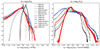 |
Fig. 1. Logarithms, f = log10(F), of volume distributions, F(μ) = dF/dμ, over the argument μ = log10(u/uB, 0), with u the energy density: of magnetic fields, uB = B2/8π (left panel), and of the plasma, upl = ⟨γ⟩nmc2 (right panel). Functions f(μ) were averaged over the duration of each simulation. |
The high-energy-density tails of the distributions have a complex structure that can be evaluated at different levels. For the reference case of σ0 = 10 without a guide field, comparing the results for simulations L1800_σ10 and L3600_σ10, convergence for FB was achieved to the level of 10−4, and for Fpl even down to 10−7. The case of σ0 = 20 is converged in Fpl down to 10−5.
2.3.1. Relaxed monster plasmoids
Monster plasmoids are very large (≳0.2L) and slow (v ≪ vA) plasmoids emerging from hierarchical mergers of plasmoids chains. In simulations performed with periodic boundary conditions, they dominate the final states into which reconnecting plasma relaxes.
The parameter with the most qualitative impact on the structure of monster plasmoids is the strength of the guide field, Bg, relative to B0. Thus, Figure 2 presents energy density maps for relaxed monster plasmoids in the final states of three simulations for Bg/B0 = 0, 0.5, 1.
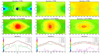 |
Fig. 2. Maps of log10(u/uB, 0)(x, y) for magnetic energy density, uB = B2/8π (upper panels), and plasma energy density, upl = ⟨γ⟩nmc2 (middle panels), for relaxed monster plasmoids at the end of each simulation. In the lower panels, we compare 1D energy density profiles of (u/uB, 0)(x, y0) measured along the strip indicated in the above maps by the dashed grey lines. A common colour scale for all maps is referenced along the left axes in the lower panels. Here, we present the effect of a guide field for σ0 = 10 and L/ρ0 = 1800. From the left, the columns show simulations: (1) L1800_σ10, (2) L1800_σ10_Bg05, and (3) L1800_σ10_Bg1. |
In the case of no guide field, Bg = 0 (L1800_σ10), the plasma energy density has a smooth structure, while the magnetic energy density ripples, especially along the x axis. The plasmoid is dominated by the plasma energy density with upl/uB ∼ 10, which peaks at μpl ≃ 0.9 across the central unmagnetised core for 0.45 < x/L < 0.54; in the fpl distribution (Figure 1, right panel, solid red line), this corresponds to a break at the −1 level. The magnetic energy density peaks at μB ≃ −0.05 (just below the initial peak of fB; Figure 1, left panel, solid red line) along a ring structure crossing the y/L = 0.75 plane at x/L ≃ 0.39 and 0.62. Hence, a relaxed monster plasmoid achieves only a minor compression of upl, and no compression of uB.
In the case of a strong guide field, Bg = B0 (L1800_σ10_Bg1), the plasmoid is characterised by a roughly uniform magnetic energy density with μB ∼ 0.3 (corresponding to the peak of fB; Figure 1, left panel, solid black line). The plasma energy density shows complex substructures, with high-density arcs tracing the magnetic field lines. Only the plasmoid core (0.4 < x/L < 0.59) is dominated by the plasma with μpl ≃ 0.6 (corresponding to a bump in fpl at the −1.1 level; Figure 1, right panel, solid black line), and hence upl/uB ∼ 2, the plasmoid layer is magnetically dominated with uB/upl ∼ 1.8.
The case of the moderate guide field, Bg = B0/2 (L1800_σ10_Bg05), shows an intermediate structure, which is qualitatively closer to the case of the strong guide field.
Figure 3 compares the y profiles of magnetic and plasma energy densities measured along the y axis of relaxed monster plasmoids. The first (from the left) panel compares such profiles for three simulation domain sizes, L/ρ0 = 900, 1800, 3600 (with no guide field, σ0 = 10). The general characteristic of these profiles (specific to the cases without a guide field) is a very sharp transition between the plasmoid core (0.455 < y/L < 0.54, uB < uB, 0/100, uniform upl) and the plasmoid layer, supported by a sharp ring structure of electric current density jz. Across the plasmoid core, the plasma energy density is roughly uniform at the level of upl ≃ 8.5uB, 0. It clearly dominates the magnetic energy density in the plasmoid layer, peaking at the level of uB, peak ≃ uB, 0, while remaining in pressure balance – a key factor is that our choice for the relativistic plasma temperature, Θe = 1, implies a relation4 between the plasma energy density and the pressure, upl/Ppl ≃ 3.4. Across the plasmoid layer, the plasma energy density decreases exponentially like upl ∝ 10−|y − y0|/(L/7), bringing the magnetic field towards the force-free equilibrium uB ∝ 1/|y − y0|2 for |y − y0|/L > 0.28. With increasing L/ρ0, the plasmoid core becomes smaller in units of L, and also larger in units of ρ0. It scales approximately as ∝(L/ρ0)1/2. However, this has little effect on the profiles of upl, both in the core and across the layer.
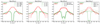 |
Fig. 3. Profiles of magnetic (green lines) and plasma (red lines) energy densities across (i.e. along the y coordinate) relaxed monster plasmoids. Panels from the left compare: (1) different sizes, L/ρ0, of simulation domain (2D with σ0 = 10, Bz = 0); (2) different magnetisations, σ0 (2D with L/ρ0 = 1800, Bz = 0); (3) 3D and 2D domains (with L/ρ0 = 900, σ0 = 10, Bz = 0); (4) different guide field strengths, Bg/B0 (2D with σ0 = 10, L/ρ0 = 1800). |
The second panel of Figure 3 compares the profiles of uB and upl for three values of initial background magnetisation σ0 = 10, 20, 40 (with no guide field, L/ρ0 = 1800). The effect of σ0 on the core and the layer of the plasmoid is rather minor (a clear effect of σ0 can be seen for y/L < 0.25 and y/L > 0.75, where background plasma still dominates). For σ0 = 10, the magnetic boundary between the core and the layer is less sharp, which is balanced by a slightly lower upl across the core.
The third panel of Figure 3 compares the profiles of uB and upl between an essentially 2D simulation (with Nz = 2) and a 3D simulation with Lz/ρ0 ≃ 42 (with Nz = 108), other key parameters being exactly the same (Lx = Ly = 900ρ0, σ0 = 10, Bg = 0). Profiles in the 3D case were calculated using different statistics along the z coordinate: minimum, mean, maximum. The resulting monster plasmoid shows a broader core with gradual boundaries – a plateau of upl ∼ 6uB, 0 with a total width of Δy ∼ 0.2L, and a base of uB ∼ 0.07uB, 0 with a total width of Δy ∼ 0.1L. The plasmoid layer is consistent between the 3D and 2D cases.
The last panel of Figure 3 compares the profiles of uB and upl for three values of the guide field strength, Bg/B0 = 0, 0.5, 1 (with L/ρ0 = 1800, σ0 = 10). In the presence of the guide field, both profiles appear less regular, which reflects a much slower relaxation of these plasma configurations. Nevertheless, one can notice that the profiles of uB are flatter, with plasmoid cores filled with uniform uB at the levels of ∼uB, 0 for Bg = B0/2, and ∼2uB, 0 for Bg = B0. Still, the plasmoid cores are dominated by upl, in the Bg = B0 case by a factor of ∼2. The plasmoid layer is roughly in equipartition for Bg = B0/2 and magnetically dominated for Bg = B0.
2.3.2. Plasmoid mergers
Figure 4 shows energy density maps for merging plasmoids in the same three simulations as in Figure 2.
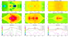 |
Fig. 4. Same as Figure 2, but for plasmoid mergers that maximise the plasma energy density, upl, for the same set of simulations: (1) L1800_σ10, (2) L1800_σ10_Bg05, and (3) L1800_σ10_Bg1. |
In the reference case L1800_σ10, the entire system of merging plasmoids including the secondary current layer is dominated by the plasma energy density reaching μpl ∼ 1.3 (corresponding to fpl ≃ −3 in the high-density tail; Figure 1, right panel, solid red line). The magnetic energy density reaches μB ∼ 0.6 (corresponding to fB ≃ −3.7; Figure 1, left panel, solid red line) in the vicinity of the current layer (possibly related to the formation of a minor secondary plasmoid). The electric energy density reaches μE ∼ −0.9 in the same region. Compared to the relaxed monster plasmoid, compression of upl is stronger by a factor of ∼2.5, but compression of uB is stronger by a factor of ∼4.5.
In the case of a strong guide field, Bg = B0 (L1800_σ10_Bg1), we show a merger that forms a secondary current layer where the plasma energy density reaches μpl ≃ 0.95 (corresponding to fpl ≃ −4; Figure 1, right panel, solid black line; higher by a factor of ≃2.2 than in the monster plasmoid) and the magnetic energy density reaches μB ≃ 0.55 (corresponding to fB ≃ −2; Figure 1, left panel, solid black line; higher by factor ≃1.8 than in the monster plasmoid).
The case of the moderate guide field, Bg = B0/2 (L1800_σ10_Bg05), shows plasma energy densities comparable to the case of no guide field.
2.3.3. Structures in the volume distributions
With this analysis, we can identify the main structures in the volume distributions fpl(μpl) and fB(μB) presented in Figure 1.
The plateau in the fpl distribution corresponds to relaxed plasmoids. In the absence of a guide field, it extends to μpl ≃ 1 or upl/uB, 0 ∼ 10, only weakly depending on the background magnetisation, σ0. Compared with the initial drifting particle population, this means a modest compression by a factor of ∼2.7. A guide field of Bz = B0 reduces this compression by a factor of ∼1.8. Such a plateau is absent in the fB distribution – relaxed plasmoids do not amplify uB.
The steep high-density tail of the fpl and fB distributions, extending to the level of −4, corresponds to plasmoid mergers. Considering the tail of the fpl distribution at the level of −4, in our reference case (σ0 = 10 in the absence of a guide field) it reaches μpl ≃ 1.5. Compared with the initial drifting particle population, this means compression by a factor of ∼8.5. A higher magnetisation of σ0 = 40 enhances this compression by a factor of ∼1.6, while a guide field of Bz = B0 reduces it by a factor of ∼3.5. Considering the tail of fB at the same level of −4, for σ0 = 10 in the absence of a guide field it reaches μB ≃ 0.75 (compression of uB, 0 by factor ∼5.5), for σ0 = 40 compression increases by a factor of ∼1.4, and for Bz = B0 it decreases by a factor of ∼1.25.
The second high-density tail of the fpl distribution, extending below the −4 level, can be identified as secondary plasmoids. Considering the level of −6, in the reference case it reaches at least μpl ≃ 2.1 (a factor ∼4 higher than for primary merging plasmoids). In the cases of σ0 = 20, 40, it reaches μpl ≃ 2.4 (factor ∼2 higher), and in the guide field case Bz = B0 it reaches μpl ≃ 1.35 (a factor of ∼5.5 lower).
2.4. Comparison with open-boundary radiative simulations
Figure 5 presents volume distributions of magnetic and plasma energy densities for simulations of relativistic reconnection initiated from a single Harris current layer using open boundary conditions and including synchrotron cooling, first presented in Ortuño-Macías & Nalewajko (2020). Open boundary conditions were applied across both ends of the current layer (x = 0 and x = Lx), which allowed for the free escape of plasmoids and prevented the formation of a single slow (due to the cancellation of x momentum) monster plasmoid. The background plasma was extended to a larger volume (Lz = 4Lx), largely preserving it in pristine condition throughout the simulation time. We thus find a stronger dominance of background plasma at uB, upl < uB, 0 (xB, xpl < 0). In the Fpl distribution, a bump for 0 < xpl < 1.1 corresponding to large plasmoids is still prominent. A major difference from periodic boundary simulations is the presence of extended power law tails in both FB and Fpl distributions. In the high-magnetisation case (σ0 = 50), the tail of FB extends over 0.3 < xB < 2.8, and the tail of Fpl extends over 1.6 < xpl < 3.7. The tails are less extended in the low-magnetisation cases (σ0 = 10), and especially the cut-off of FB is sensitive to radiative cooling efficiency, shifting to xB ≃ 1.2 for Θ = 2 × 10⁵ (slow cooling). The power law index is approximately p ≃ −5/3 for both FB and Fpl, although for σ0 = 50 it hardens towards the highest xB, xpl to p ≃ −1, and for σ0 = 10 it softens to p ≃ −2.
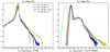 |
Fig. 5. Same as Figure 1, but for the open-boundary simulations with synchrotron cooling first presented in Ortuño-Macías & Nalewajko (2020). The black dashed lines indicate power laws of index −5/3. |
3. Relativistic jets
Relativistic jets are launched from rotating magnetospheres with large fluxes in the poloidal magnetic field (Blandford 1976). The twist of the poloidal magnetic field generates a toroidal magnetic component and a perpendicular electric field, combining into outflowing electromagnetic momentum – the Poynting flux. In the process of Blandford & Znajek (1977), an electromagnetic version of the Penrose process (Lasota et al. 2014), torque is exerted on the BH, converting its rotational energy to the energy of the toroidal magnetic field and the associated electric field.
A magnetosphere connected to the BH horizon achieves highly relativistic magnetisation (σ = b2/w ≫ 1) and force-free conditions (negligible inertia, ρc2, pressure, P, enthalpy, w; sufficient charge density, ρe, current density, j) by unloading its plasma onto the BH. This results in a sharply edged cavity of low plasma density, which (in combination with relatively uniform magnetic enthalpy density, b2) corresponds with the σ > 1 magnetosphere (e.g. Nalewajko et al. 2024).
An outflowing BH magnetosphere is gradually collimated by external plasma pressure and accelerated by the pressure of the toroidal magnetic field (Camenzind 1989), converting its electromagnetic energy into kinetic plasma energy. According to the conservation of the Michel parameter (specific energy) μ = Γ(1 + σϕ′) (Michel 1969), magnetisation σϕ′=Bϕ′2/(4πw′), based on the co-moving toroidal magnetic field Bϕ′ and relativistic enthalpy density w′, converts into the bulk Lorentz factor Γ. The efficiency of such acceleration depends critically on the geometry of poloidal magnetic field lines – it is particularly low in the spherical case (Begelman & Li 1994), but can be very high in the parabolic case (Beskin & Nokhrina 2006). In this acceleration-collimation zone (ACZ), extending to distances of r (103 − 105)MBH (Komissarov et al. 2007, 2009), the jet is characterised by high magnetisation and largely ordered magnetic fields.
The boundary of a relativistic jet can be defined by the trans-relativistic four-velocity u = Γv/c = 1, which corresponds to the Lorentz factor  . Within the jet is the density cavity, which in the ACZ can be identified by σ = 1 (beyond the ACZ, σ < 1 across the entire jet; whether the cavity remains well defined depends on the efficiency of plasma mixing processes). Recent numerical works (e.g. Davelaar et al. 2018; Salas et al. 2024) describe the inner σ > 1 region as the jet spine, and the outer σ < 1 region as the jet sheath; the original spine-sheath structure was proposed by Ghisellini et al. (2005).
To describe the jet structure, we use spherical coordinates (r, θ, ϕ) and a cylindrical radius of R = r sin θ. Gradual collimation in the ACZ means that the shape of the jet spine, θsp(r), can be described as paraboloidal. Beyond the ACZ, it transitions to conical; this has been confirmed by direct measurements of the innermost jets in nearby AGNs with the very-long-baseline interferometry (VLBI) technique (Asada & Nakamura 2012; Kovalev et al. 2020). A flat or slowly declining profile of external (sheath) pressure may even lead to recollimation of the jet spine (Bromberg & Levinson 2007; Porth & Komissarov 2015).
3.1. Lateral structure of jet magnetic fields
Relativistic jets can be robustly described by stationary and axisymmetric models. In such models, one considers two main components of the magnetic and velocity fields that are closely interrelated. The poloidal plasma velocity is parallel to the poloidal magnetic field; hence, poloidal plasma streamlines θs(r) coincide with the poloidal field lines. The relation between the poloidal and toroidal magnetic fields is governed by the trans-field momentum (Grad-Shafranov) equation (Beskin 2010). Detailed solutions presented in the literature (e.g. Appl & Camenzind 1993; Lyubarsky 2009, 2010; Beskin et al. 2023) show several characteristic features. One can start by describing the poloidal component, persistently anchored to the central engine, and then discuss the toroidal component as a train of giant electromagnetic waves propagating along the poloidal streamlines.
Close to the BH, the magnetosphere is uncollimated; hence, the streamlines are roughly spherical, θs(r)≃θs(rH). In the initial stage of uniform (equilibrium) collimation (Lyubarsky 2010), the entire jet remains in causal contact, and the streamlines are able to adapt to the jet spine boundary, θsp(r), to the tension of toroidal magnetic field, and to the centrifugal forces due to both azimuthal rotation and poloidal curvature (Narayan et al. 2009). In the subsequent stage of differential (non-equilibrium) collimation, beyond the fast magnetosonic surface, the inner layer of poloidal field lines bunches towards the jet symmetry axis (Tchekhovskoy et al. 2009; Chatterjee et al. 2019). An important consequence is that the strength of poloidal magnetic field, Bp, evolves very differently along individual field lines.
Close to the jet symmetry axis, magneto-hydrodynamic (MHD) models predict a narrow cylindrical structure called the jet core (e.g. Appl & Camenzind 1993; Beskin & Nokhrina 2009; Lyubarsky 2009; Beskin et al. 2023). Here, the poloidal magnetic field lines are able, more or less, to co-rotate at the rate imposed by the central engine (this corresponds roughly to the light cylinder of pulsars). The characteristic radius of the jet core is Rc ∼ uc/ΩB, where uc = Γcβc ∼ 1 is the minimal four-velocity of bulk motion along the core5. For a ≃ 0.9, this means that Rc ≃ 6MBH, effectively imposing the BH length scale over great distances. A strictly cylindrical jet core would maintain constant Bp, support only a weak toroidal field (hence little Poynting flux), and inefficient bulk acceleration with Γj ≃ Bϕ/Bp ≃ ΩBR (Lyubarsky 2009).
Outside the jet core (R > Rc), differential collimation results in poloidal field lines diverging faster than in the spherical case, resulting in Bp declining steeper than 1/r2, enhancing the acceleration efficiency due to the magnetic nozzle effect (Begelman & Li 1994). Efficient conversion of magnetic to kinetic energy still requires maintaining equilibrium with the external pressure (Lyubarsky 2010). On the other hand, a steeply decreasing external pressure (e.g. when a gamma-ray burst jet breaks out of a collapsar) enables additional acceleration of the outermost jet layers via the rarefaction mechanism (Tchekhovskoy et al. 2010; Komissarov et al. 2010).
The toroidal magnetic field is induced by the rotation of poloidal field lines at the jet base, where the centrifugal force wins over BH gravity and dominates the magnetic tension. Black hole magnetospheres do not rotate rigidly, and they inject the toroidal field over a broad range of streamlines, well away from the jet core. The relative strengths of the toroidal and poloidal components define the magnetic pitch, 𝒫 = RBr/Bϕ (Appl et al. 2000; Bromberg et al. 2019). The initial stage of jet collimation is characterised by roughly uniform 𝒫. At the jet core radius, Rc, one has Bϕ ≃ Br; hence, 𝒫 ≃ Rc across the jet. This implies that radial profiles of toroidal field strength Bϕ(R) peak well outside the jet core, and hence Rc is not their characteristic lateral scale.
(Chatterjee et al. 2019) performed axisymmetric general-relativistic MHD (GRMHD) simulations of strongly collimated relativistic jets extending to distances beyond 105rg. They demonstrated strong bunching of poloidal field lines (Tchekhovskoy et al. 2009) leading to the formation of a jet core with a radius of Rc ≃ 4RL (Beskin et al. 2023) (their a = 15/16 implies ΩB ≃ ΩH/2 ≃ 0.17; hence, RL ≃ 5.7Rg). On the one hand, bunching of poloidal field lines is a consequence of the magnetic tension of the toroidal field; on the other hand, bunched poloidal field lines transmit the toroidal field parallel to the jet core. The toroidal magnetic energy gradually converts into the kinetic energy of the plasma, resulting in high bulk Lorentz factors in the vicinity of the jet core, which was also reported by Chatterjee et al. (2019). At the same time, the outer jet regions are loaded with denser proton plasma from the sheath region, apparently due to the interchange (magnetic Rayleigh-Taylor) instability6. Mass loading via instabilities is expected to develop a highly inhomogeneous filamentary structure; whether such filaments can reach the jet core is unknown. It has been suggested that filamentary mass loading would result in highly inhomogeneous jet magnetisation with σmax ≳ 103 matching the maximum particle energies inferred from non-thermal emission of blazars (Nalewajko 2016). On average, mass loading should reduce not only the bulk Lorentz factor, Γ, but also the Michel parameter, μ = Γ(1 + σ) (maximum achievable Γ, hence the potential for further acceleration). The overall effect of poloidal field bunching is thus the concentration of the jet energy flux along the jet core.
The poloidal pressure of the toroidal magnetic field is the main force accelerating the jet to relativistic speeds. A non-uniform structure of Bϕ(θ) results in a non-uniform structure of Γ(θ). The acceleration efficiency depends also on the geometry of jet streamlines (the rate of velocity divergence). Thus, acceleration should be less efficient in the jet core, and particularly along the jet axis. The toroidal magnetic field is the main carrier of the poloidal Poynting flux, which is converted into plasma kinetic energy density along each streamline.
The lateral structure of a relativistic jet spine in the differentiated ACZ stage is summarised schematically in Figure 6. Across such a jet spine, we distinguish three zones: the innermost cylindrical jet core, the intermediate quasi-cylindrical bunched spine, and the outermost paraboloidal main spine. The bunched spine is distinguished as the location of the peak bulk Lorentz factor, Γ, and the toroidal magnetic field, Bϕ, which means the peak energy (Poynting) flux density. The main spine zone is the most extended and carries the bulk of the energy flux. It can be polluted by protons from the jet sheath via boundary instabilities (Chatterjee et al. 2019), but this reduces the bulk Lorentz factor and dilutes the energy flux density. The jet core is prone to current-driven instability (CDI) (Kruskal & Schwarzschild 1954; Freidberg 1982; Begelman 1998), which can accelerate particles via reconnection in high-σ conditions (Alves et al. 2018; Davelaar et al. 2020; Ortuño-Macías et al. 2022). However, the reduced bulk Lorentz factor of the jet core would reduce the relativistic boost of associated radiation.
 |
Fig. 6. Proposed lateral structure (not to scale) of a relativistic jet differentiated due to poloidal field bunching. The ‘bunched spine’ zone is introduced as the region maximizing the jet energy flux density. The introduction of plasmoids from reconnection layers created due to CDI in the jet core allow the energy density enhancement factors of the plasmoids and of the bunched jet spine to multiply. |
Efficient poloidal field bunching would result in a narrow bunched spine with a radius of peak toroidal field strength Rpeak ≪ Rj. It also implies the enhancement of the peak Poynting flux density, S, compared with the mean value across the jet spine. In Appendix C, we consider a generic model for radial profiles S(R) and calculate the dependence between the enhancement factor fS = Speak/⟨ S⟩ and Rpeak/Rj. We find that fS ∝ (Rpeak/Rj)−3/2, for example enhancement by a factor of fS ∼ 10, requires Rpeak/Rj ∼ 0.15.
In numerical simulations of the CDI, perturbations tend to spread from the most unstable toroidal field core to the outside (Bromberg & Tchekhovskoy 2016; Bromberg et al. 2019; Ortuño-Macías et al. 2022). Hence, we propose that plasmoids from reconnection layers induced by CDI in the jet core may spread to the bunched spine zone, as is indicated in Figure 6. During that process, they would be need to be carried by the poloidal bulk flow of the jet in order to relativistically boost the emitted radiation. Carrying large plasmoids by background high-σ flow is not expected to be a highly efficient process, because of their significant inertia, which in a slightly different context results in an anti-correlation between plasmoid growth and bulk acceleration (Sironi et al. 2016; Ortuño-Macías & Nalewajko 2020). Moreover, the poloidal velocity shear is rarely accounted for in studies of CDI (Nalewajko & Begelman 2012), and its effect is still unclear. Alternatively, strongly sheared magnetic perturbations may induce reconnection layers directly in the bunched spine zone.
4. Discussion and conclusions
We considered an analogy between the lateral structures of relativistic jets and plasmoids produced by magnetic reconnection. In both cases, a key role is played by the toroidal component of magnetic field, the tension of which introduces an anisotropic stress that in principle can compress the energy density of both plasma and the magnetic field.
Compression of the energy density in reconnection plasmoids was investigated by kinetic PIC numerical simulations in 2D and 3D periodic domains, starting from hot Harris layers and evolving to relaxed monster plasmoids. We considered the effects of domain size, background magnetisation, and the guide magnetic field. In our simulations without a guide field, the plasma energy density achieves values of upl ∼ 102uB, 0 (relative to the initial background magnetic energy density), higher than the magnetic energy density, uB ∼ 10uB, 0. The highest energy densities correspond to the secondary plasmoids emerging between merging primary plasmoids. However, the initial plasma energy density extends to ∼4uB, 0 for the hot drifting particles. In the presence of a guide field or third dimension, the plasma energy densities are reduced by a few factors.
We have also re-analysed the results of previous PIC simulations, first presented in Ortuño-Macías & Nalewajko (2020), which used open boundaries and synchrotron cooling. Those results show power law tails in the distributions of both upl and uB with indices close to −5/3. The cooling efficiency affects mainly the extent of the uB distribution, which may explain the apparent lack of such a power law tail in the results of our new simulations.
In relativistic jets, the effect of the toroidal magnetic field has been controversial. Eventually, it was understood that its tension is insufficient to collimate such jets. However, toroidal field tension has the subtle effect of gradually differentiating the lateral jet structure. The key effect of poloidal field bunching has been identified by Tchekhovskoy et al. (2009). We propose that this effect forms an intermediate layer across the jet spine, referred to as the bunched spine, adjacent to the central jet core, corresponding roughly to the peaks of both the toroidal field strength, Bϕ(R), and the bulk Lorentz factor, Γ(R). The bunched spine is characterised by an enhanced Poynting flux density, S. For generic radial profiles of S(R), the enhancement factor, fS = Speak/⟨ S⟩, is sensitive to the relative peak radius, Rpeak/Rj. Poloidal field bunching was demonstrated in 2D GRMHD global simulations of relativistic jets (Chatterjee et al. 2019); however, it appears to be less efficient in 3D simulations.
An additional enhancement of the luminosity of short flares of energetic radiation can be provided by the effect of kinetic beaming (Cerutti et al. 2012), also known as pitch-angle anisotropy (Comisso & Sironi 2021; Sobacchi et al. 2023). This effect is not expected to be important in relaxed reconnection plasmoids, but rather during the formation of plasmoid chains, and likely also during plasmoid mergers. Our PIC simulations confirm that plasmoid mergers produce the highest energy densities in reconnection layers, and the resulting radiation intensity could be further enhanced by kinetic beaming.
The possibility of locally concentrating the momentum flux density of relativistic jets is important also for alternative models of rapid blazar flares; for example, the obliteration of stars wandering into the jet (e.g. Bednarek & Protheroe 1997). The efficiency of bulk acceleration can be increased in a sharply inhomogeneous jet due to impulsive acceleration (Granot et al. 2011), which can also be described as a relativistic whip.
4.1. The jet of M87
The proposed scenario can be confronted with observations of relativistic AGN jets resolved by VLBI. In the best-studied case of M87 (for review see Hada et al. 2024), the approaching jet (seen at the viewing angle of ≃18°) has long been known to be limb-brightened at scales7 of ∼50 mas (Reid et al. 1989), ∼1 mas (Junor et al. 1999), and ∼0.2 mas (Kim et al. 2018). The < 0.6 mas limbs were modelled by Punsly (2022, 2023, 2024) in terms of the thick tubular jet sheath. Recently, a third central ridge has been reported on scales of ∼0.5 mas (Lu et al. 2023) and ∼8 mas (Tazaki et al. 2023), and possibly also at ∼300 mas8. The 0.5 mas ridge was interpreted by Lyutikov & Ibrahim (2024) in terms of strong beaming due to the instant bulk acceleration of a pair-dominated hollow-cone jet. The central ridge appears more likely to be a signature of the jet core weakly beamed due to a reduced bulk Lorentz factor. The highly relativistic jet spine would be de-beamed at such a large viewing angle.
According to the AGN unification paradigm (Urry & Padovani 1995), a Fanaroff-Riley type I radio galaxy such as M87 should be a misaligned counterpart of a BL Lac type blazar. Beamed non-thermal blazar emission should be produced in a highly dissipative blazar zone. Models of BL Lac type blazars do not provide strong constraints on the location. A de-projected distance of 1 pc corresponds to ≃4 mas, indicating that the ∼8 mas ridge is potentially adjacent to a blazar zone in the form of bunched spine.
A well known dissipative zone in the M87 jet is the HST-1 knot observed at ≃860 mas (Giroletti et al. 2012). It shows evidence of apparently superluminal motions (Biretta et al. 1999; Cheung et al. 2007), and produced a spectacular X-ray/optical/radio outburst over a timescale of a few years (e.g. Harris et al. 2006, 2009). It has been suggested to be the blazar zone of the M87 jet (Barnacka et al. 2014), which would pose severe problems of sufficient energy density and a short variability timescale at a de-projected distance of ∼220 pc.
4.2. Conclusions
In the multi-scale system of a relativistic jet hosting plasmoids produced by magnetic reconnection, we consider it more likely for a significant (factor ≳10) energy density enhancement to be achieved due to tension of the toroidal magnetic field on the local scale of plasmoid cores, rather than on the global scale of a bunched jet spine (the layer adjacent to the central jet core). Even a moderate (∼3) global-scale enhancement combined with a stronger (∼10) local-scale enhancement would boost the luminosity of rapid blazar flares by a factor of ∼30 at standard jet bulk Lorentz factors of Γj ∼ 10 − 20, strongly reducing the extreme energetic requirements of such flares.
However, even for the brightest blazar flares detected in γ-rays by the Fermi satellite, the statistical significance of variability on suborbital timescales (typically within ∼30 min windows) is limited to ∼2σ (Meyer et al. 2019); see also Nalewajko (2017).
However, it has been argued that relativistic turbulence provides more consistent beaming statistics than minijets (Narayan & Piran 2012; Sobacchi et al. 2023).
Subscripts 0 refer to the background plasma.
For isotropic Maxwell-Jüttner distribution, upl/Ppl equals the mean particle Lorentz factor ⟨γ⟩ ≃ 3Θe + K1(1/Θe)/K2(1/Θe), with Kn the modified Bessel function of the second kind.
For a Kerr BH of mass MBH and spin a in natural units G = c = 1, the outer horizon radius is rH/MBH = 1 + (1 − a2)1/2, and the angular velocity is ΩH = a/(2rH). The magnetosphere rotates with an angular velocity of ΩB ≃ ΩH/2 (Komissarov 2001).
Chatterjee et al. (2019) call this a pinch instability, with ‘pinch’ referring to longitudinal ∝exp(ikr) perturbations of the spine-sheath boundary; ‘pinch’ usually refers to the m = 0 mode of current-driven perturbations, ∝exp(imϕ).
At the estimated distance of DM87* ≃ 16.8 Mpc and BH mass MM87* ≃ 6.5 × 10⁹ M⊙ (Event Horizon Telescope Collaboration 2019), 1 mas corresponds to a projected linear scale of ≃81 mpc ≡ 260Rg, and a de-projected scale of ≃0.26 pc.
Presented by T. Savolainen at the IAU Symposium 375 in Kathmandu, Nepal (Dec. 2022).
Propagating pattern, rather than stationary (Sikora et al. 1997).
Corresponding to the magnetic jet power of PB = (c/8)(ΓjRjB′)2 ∼ 1044 erg s−1.
Acknowledgments
We gratefully acknowledge Poland’s high-performance Infrastructure PLGrid (HPC Centers: ACK Cyfronet AGH, PCSS, CI TASK, WCSS) for providing computer facilities and support within computational grants no. PLG/2023/016444 and PLG/2024/017356; and the Nicolaus Copernicus Astronomical Center for providing the Chuck cluster. This work was supported by the Polish National Science Centre grant 2021/41/B/ST9/04306.
References
- Abdo, A. A., Ackermann, M., Ajello, M., et al. 2011, ApJ, 733, L26 [NASA ADS] [CrossRef] [Google Scholar]
- Ackermann, M., Anantua, R., Asano, K., et al. 2016, ApJ, 824, L20 [NASA ADS] [CrossRef] [Google Scholar]
- Aharonian, F., Akhperjanian, A. G., Bazer-Bachi, A. R., et al. 2007, ApJ, 664, L71 [NASA ADS] [CrossRef] [Google Scholar]
- Alves, E. P., Zrake, J., & Fiuza, F. 2018, Phys. Rev. Lett., 121, 245101 [NASA ADS] [CrossRef] [Google Scholar]
- Appl, S., & Camenzind, M. 1993, A&A, 274, 699 [NASA ADS] [Google Scholar]
- Appl, S., Lery, T., & Baty, H. 2000, A&A, 355, 818 [NASA ADS] [Google Scholar]
- Asada, K., & Nakamura, M. 2012, ApJ, 745, L28 [NASA ADS] [CrossRef] [Google Scholar]
- Barnacka, A., Geller, M. J., Dell’Antonio, I. P., et al. 2014, ApJ, 788, 139 [NASA ADS] [CrossRef] [Google Scholar]
- Bednarek, W., & Protheroe, R. J. 1997, MNRAS, 287, L9 [NASA ADS] [CrossRef] [Google Scholar]
- Begelman, M. C. 1998, ApJ, 493, 291 [NASA ADS] [CrossRef] [Google Scholar]
- Begelman, M. C., & Li, Z.-Y. 1994, ApJ, 426, 269 [NASA ADS] [CrossRef] [Google Scholar]
- Begelman, M. C., Blandford, R. D., & Rees, M. J. 1984, RvMP, 56, 255 [Google Scholar]
- Beskin, V. S. 2010, MHD Flows in Compact Astrophysical Objects: Accretion, Winds and Jets (Berlin, Heidelberg: Springer-Verlag), Astron. Astrophys. Lib., ISBN 978-3-642-01289-1, 2010 [Google Scholar]
- Beskin, V. S., & Nokhrina, E. E. 2006, MNRAS, 367, 375 [Google Scholar]
- Beskin, V. S., & Nokhrina, E. E. 2009, MNRAS, 397, 1486 [NASA ADS] [CrossRef] [Google Scholar]
- Beskin, V. S., Kniazev, F. A., & Chatterjee, K. 2023, MNRAS, 524, 4012 [Google Scholar]
- Beskin, V. S., Khalilov, T. I., Nokhrina, E. E., et al. 2024, MNRAS, 528, 6046 [NASA ADS] [CrossRef] [Google Scholar]
- Biretta, J. A., Sparks, W. B., & Macchetto, F. 1999, ApJ, 520, 621 [NASA ADS] [CrossRef] [Google Scholar]
- Blandford, R. D. 1976, MNRAS, 176, 465 [NASA ADS] [Google Scholar]
- Blandford, R. D., & Znajek, R. L. 1977, MNRAS, 179, 433 [NASA ADS] [CrossRef] [Google Scholar]
- Blandford, R., Meier, D., & Readhead, A. 2019, ARA&A, 57, 467 [NASA ADS] [CrossRef] [Google Scholar]
- Bromberg, O., & Levinson, A. 2007, ApJ, 671, 678 [NASA ADS] [Google Scholar]
- Bromberg, O., & Tchekhovskoy, A. 2016, MNRAS, 456, 1739 [CrossRef] [Google Scholar]
- Bromberg, O., Singh, C. B., Davelaar, J., et al. 2019, ApJ, 884, 39 [NASA ADS] [Google Scholar]
- Camenzind, M. 1989, Accretion Disks and Magnetic Fields in Astrophysics, 156, 129 [NASA ADS] [Google Scholar]
- Cerutti, B., Werner, G. R., Uzdensky, D. A., et al. 2012, ApJ, 754, L33 [NASA ADS] [CrossRef] [Google Scholar]
- Cerutti, B., Werner, G. R., Uzdensky, D. A., & Begelman, M. C. 2013, ApJ, 770, 147 [Google Scholar]
- Chatterjee, K., Liska, M., Tchekhovskoy, A., et al. 2019, MNRAS, 490, 2200 [NASA ADS] [CrossRef] [Google Scholar]
- Chernoglazov, A., Hakobyan, H., & Philippov, A. 2023, ApJ, 959, 122 [NASA ADS] [CrossRef] [Google Scholar]
- Cheung, C. C., Harris, D. E., & Stawarz, Ł. 2007, ApJ, 663, L65 [NASA ADS] [CrossRef] [Google Scholar]
- Christie, I. M., Petropoulou, M., Sironi, L., et al. 2019, MNRAS, 482, 65 [NASA ADS] [CrossRef] [Google Scholar]
- Clausen-Brown, E., Savolainen, T., Pushkarev, A. B., et al. 2013, A&A, 558, A144 [NASA ADS] [CrossRef] [EDP Sciences] [Google Scholar]
- Comisso, L., & Sironi, L. 2021, Phys. Rev. Lett., 127, 255102 [Google Scholar]
- Davelaar, J., Mościbrodzka, M., Bronzwaer, T., et al. 2018, A&A, 612, A34 [NASA ADS] [CrossRef] [EDP Sciences] [Google Scholar]
- Davelaar, J., Philippov, A. A., Bromberg, O., et al. 2020, ApJ, 896, L31 [NASA ADS] [CrossRef] [Google Scholar]
- Davis, S. W., & Tchekhovskoy, A. 2020, ARA&A, 58, 407 [Google Scholar]
- Event Horizon Telescope Collaboration (Akiyama, K., et al.) 2019, ApJ, 875, L6 [Google Scholar]
- Freidberg, J. P. 1982, RvMP, 54, 801 [Google Scholar]
- Furth, H. P., Killeen, J., & Rosenbluth, M. N. 1963, PhFl, 6, 459 [NASA ADS] [Google Scholar]
- Ghisellini, G., Tavecchio, F., & Chiaberge, M. 2005, A&A, 432, 401 [CrossRef] [EDP Sciences] [Google Scholar]
- Giannios, D. 2013, MNRAS, 431, 355 [NASA ADS] [CrossRef] [Google Scholar]
- Giannios, D., Uzdensky, D. A., & Begelman, M. C. 2009, MNRAS, 395, L29 [NASA ADS] [CrossRef] [Google Scholar]
- Giroletti, M., Hada, K., Giovannini, G., et al. 2012, A&A, 538, L10 [NASA ADS] [CrossRef] [EDP Sciences] [Google Scholar]
- Granot, J., Komissarov, S. S., & Spitkovsky, A. 2011, MNRAS, 411, 1323 [NASA ADS] [CrossRef] [Google Scholar]
- Hada, K., Asada, K., Nakamura, M., et al. 2024, A&ARv, 32, 5 [NASA ADS] [Google Scholar]
- Hakobyan, H., Petropoulou, M., Spitkovsky, A., et al. 2021, ApJ, 912, 48 [NASA ADS] [CrossRef] [Google Scholar]
- Hakobyan, H., Ripperda, B., & Philippov, A. A. 2023, ApJ, 943, L29 [Google Scholar]
- Harris, D. E., Cheung, C. C., Biretta, J. A., et al. 2006, ApJ, 640, 211 [NASA ADS] [CrossRef] [Google Scholar]
- Harris, D. E., Cheung, C. C., Stawarz, Ł., et al. 2009, ApJ, 699, 305 [NASA ADS] [CrossRef] [Google Scholar]
- Jorstad, S. G., Marscher, A. P., Mattox, J. R., et al. 2001, ApJS, 134, 181 [Google Scholar]
- Junor, W., Biretta, J. A., & Livio, M. 1999, Nature, 401, 891 [NASA ADS] [CrossRef] [Google Scholar]
- Kim, J.-Y., Krichbaum, T. P., Lu, R.-S., et al. 2018, A&A, 616, A188 [NASA ADS] [CrossRef] [EDP Sciences] [Google Scholar]
- Kirk, J. G., & Skjæraasen, O. 2003, ApJ, 591, 366 [CrossRef] [Google Scholar]
- Komissarov, S. S. 2001, MNRAS, 326, L41 [Google Scholar]
- Komissarov, S. S., Barkov, M. V., Vlahakis, N., et al. 2007, MNRAS, 380, 51 [NASA ADS] [CrossRef] [Google Scholar]
- Komissarov, S. S., Vlahakis, N., Königl, A., et al. 2009, MNRAS, 394, 1182 [NASA ADS] [CrossRef] [Google Scholar]
- Komissarov, S. S., Vlahakis, N., & Königl, A. 2010, MNRAS, 407, 17 [NASA ADS] [CrossRef] [Google Scholar]
- Kovalev, Y. Y., Pushkarev, A. B., Nokhrina, E. E., et al. 2020, MNRAS, 495, 3576 [NASA ADS] [CrossRef] [Google Scholar]
- Kruskal, M., & Schwarzschild, M. 1954, RSPSA, 223, 348 [Google Scholar]
- Lasota, J.-P., Gourgoulhon, E., Abramowicz, M., et al. 2014, Phys. Rev. D, 89, 024041 [NASA ADS] [CrossRef] [Google Scholar]
- Lister, M. L., Aller, M. F., Aller, H. D., et al. 2016, AJ, 152, 12 [NASA ADS] [CrossRef] [Google Scholar]
- Loureiro, N. F., Schekochihin, A. A., & Cowley, S. C. 2007, PhPl, 14, 100703 [NASA ADS] [Google Scholar]
- Lu, R.-S., Asada, K., Krichbaum, T. P., et al. 2023, Nature, 616, 686 [CrossRef] [Google Scholar]
- Lyubarsky, Y. 2009, ApJ, 698, 1570 [NASA ADS] [CrossRef] [Google Scholar]
- Lyubarsky, Y. E. 2010, MNRAS, 402, 353 [Google Scholar]
- Lyutikov, M., & Ibrahim, A. 2024, ApJ, 962, 18 [NASA ADS] [Google Scholar]
- Madejski, G., & Sikora, M. 2016, ARA&A, 54, 725 [NASA ADS] [CrossRef] [Google Scholar]
- Meyer, M., Scargle, J. D., & Blandford, R. D. 2019, ApJ, 877, 39 [Google Scholar]
- Michel, F. C. 1969, ApJ, 158, 727 [NASA ADS] [CrossRef] [Google Scholar]
- Morris, P. J., Potter, W. J., & Cotter, G. 2019, MNRAS, 486, 1548 [NASA ADS] [CrossRef] [Google Scholar]
- Nalewajko, K. 2016, Galaxies, 4, 28 [NASA ADS] [CrossRef] [Google Scholar]
- Nalewajko, K. 2017, Galaxies, 5, 100 [NASA ADS] [CrossRef] [Google Scholar]
- Nalewajko, K., & Begelman, M. C. 2012, MNRAS, 427, 2480 [CrossRef] [Google Scholar]
- Nalewajko, K., Giannios, D., Begelman, M. C., et al. 2011, MNRAS, 413, 333 [NASA ADS] [CrossRef] [Google Scholar]
- Nalewajko, K., Begelman, M. C., Cerutti, B., et al. 2012, MNRAS, 425, 2519 [NASA ADS] [CrossRef] [Google Scholar]
- Nalewajko, K., Begelman, M. C., & Sikora, M. 2014, ApJ, 789, 161 [NASA ADS] [Google Scholar]
- Nalewajko, K., Uzdensky, D. A., Cerutti, B., et al. 2015, ApJ, 815, 101 [NASA ADS] [CrossRef] [Google Scholar]
- Nalewajko, K., Kapusta, M., & Janiuk, A. 2024, A&A, 692, A37 [NASA ADS] [CrossRef] [EDP Sciences] [Google Scholar]
- Narayan, R., & Piran, T. 2012, MNRAS, 420, 604 [NASA ADS] [CrossRef] [Google Scholar]
- Narayan, R., Li, J., & Tchekhovskoy, A. 2009, ApJ, 697, 1681 [NASA ADS] [CrossRef] [Google Scholar]
- Ortuño-Macías, J., & Nalewajko, K. 2020, MNRAS, 497, 1365 [Google Scholar]
- Ortuño-Macías, J., Nalewajko, K., Uzdensky, D. A., et al. 2022, ApJ, 931, 137 [Google Scholar]
- Parker, E. N. 2007, Conversations on Electric and Magnetic Fields in the Cosmos (Princeton: Princeton University Press), ISBN-10 0-691-12840-5 (HB) [Google Scholar]
- Petropoulou, M., & Sironi, L. 2018, MNRAS, 481, 5687 [NASA ADS] [CrossRef] [Google Scholar]
- Petropoulou, M., Giannios, D., & Sironi, L. 2016, MNRAS, 462, 3325 [NASA ADS] [CrossRef] [Google Scholar]
- Porth, O., & Komissarov, S. S. 2015, MNRAS, 452, 1089 [Google Scholar]
- Punsly, B. 2022, ApJ, 936, 79 [NASA ADS] [CrossRef] [Google Scholar]
- Punsly, B. 2023, A&A, 679, L1 [NASA ADS] [CrossRef] [EDP Sciences] [Google Scholar]
- Punsly, B. 2024, A&A, 685, L3 [NASA ADS] [CrossRef] [EDP Sciences] [Google Scholar]
- Reid, M. J., Biretta, J. A., Junor, W., et al. 1989, ApJ, 336, 112 [NASA ADS] [CrossRef] [Google Scholar]
- Ripperda, B., Liska, M., Chatterjee, K., et al. 2022, ApJ, 924, L32 [NASA ADS] [CrossRef] [Google Scholar]
- Salas, L. D. S., Musoke, G., Chatterjee, K., et al. 2024, MNRAS, 533, 254 [NASA ADS] [CrossRef] [Google Scholar]
- Schoeffler, K. M., Grismayer, T., Uzdensky, D., et al. 2023, MNRAS, 523, 3812 [NASA ADS] [CrossRef] [Google Scholar]
- Shukla, A., & Mannheim, K. 2020, NatCo, 11, 4176 [Google Scholar]
- Sikora, M., Madejski, G., Moderski, R., et al. 1997, ApJ, 484, 108 [CrossRef] [Google Scholar]
- Sironi, L., Petropoulou, M., & Giannios, D. 2015, MNRAS, 450, 183 [Google Scholar]
- Sironi, L., Giannios, D., & Petropoulou, M. 2016, MNRAS, 462, 48 [NASA ADS] [CrossRef] [Google Scholar]
- Sobacchi, E., Piran, T., & Comisso, L. 2023, ApJ, 946, L51 [NASA ADS] [Google Scholar]
- Tazaki, F., Cui, Y., Hada, K., et al. 2023, Galaxies, 11, 39 [NASA ADS] [CrossRef] [Google Scholar]
- Tchekhovskoy, A., McKinney, J. C., & Narayan, R. 2009, ApJ, 699, 1789 [NASA ADS] [CrossRef] [Google Scholar]
- Tchekhovskoy, A., Narayan, R., & McKinney, J. C. 2010, New Astron., 15, 749 [NASA ADS] [CrossRef] [Google Scholar]
- Urry, C. M., & Padovani, P. 1995, PASP, 107, 803 [NASA ADS] [CrossRef] [Google Scholar]
- Zhang, H., Dong, L., & Giannios, D. 2024, MNRAS, 531, 4781 [NASA ADS] [CrossRef] [Google Scholar]
Appendix A: Energetics of blazar flares
Rapid and luminous blazar flares require efficient conversion of very high energy densities. For a typical estimate, consider a compact flaring region of radius Rfl′ propagating with speed βfl = vfl/c and Lorentz factor Γfl = (1 − βfl2)−1/2 (defining reference frame 𝒪′), and observed at viewing angle θobs ≃ 1/Γfl corresponding to a Doppler factor 𝒟fl = [Γfl(1 − βfl cos θobs)]−1 ∼ Γfl resulting in a luminosity boost9Lfl, obs = 𝒟fl4Lfl′ and shortening of variability timescale tfl = tfl′/𝒟fl. In blazars, relativistic motions with bulk Lorentz factors Γfl ∼ 20 can be deduced from apparently superluminal proper motions with speeds vapp ∼ 20c (with c the speed of light) along the jet (e.g. Jorstad et al. 2001; Lister et al. 2016). The intrinsic parameters can be approximated as tfl′∼Rfl′/c and Lfl′∼4πRfl′2ufl′c with ufl′ the intrinsic radiation energy density. The total power carried by the flare photons can be estimated as Pfl ∼ πRfl2Γfl2ufl′c ∼ [Γfl2/(4𝒟fl4)]Lfl, obs ∼ Lfl, obs/(4Γfl2) with Rfl = Rfl′∼𝒟flctfl. That power can be compared with the Eddington luminosity of the supermassive BH LEdd ≃ 1.5 × 1047(MBH/109 M⊙) erg/s with MBH ∼ 109 M⊙ the BH mass in units of the solar mass M⊙. For flaring FSRQs this gives Pfl, FSRQ ∼ 0.4(Γfl/20)−2LEdd, which is dangerously close to LEdd, and this is one reason to consider significantly higher values of Γfl (Ackermann et al. 2016). For flaring HBLs, Pfl, HBL ∼ 4 × 10⁻⁴(Γfl/20)−2LEdd, more comfortable at least in terms of LEdd.
Consider that this compact blazar zone is only a small part of a relativistic jet with a total power Pj and Lorentz factor Γj. At distance scale r the jet has lateral radius Rj = θjr with θj the half-opening angle. Interferometric radio observations of pc-scale blazar jets suggest that Γjθj ∼ 0.2 (Clausen-Brown et al. 2013). The jet can be subdivided laterally into streamtubes, of which we are interested only in the streamtube of radius Rst = Rfl that completely and minimally contains the flaring region. Neglecting the poloidal line bunching and assuming that power per unit solid-angle is roughly uniform across the jet, the fraction of jet power Pst in that streamtube would scale as Pst/Pj ≃ (Rst/Rj)2. We can ask, at what distances is the jet power passing through a flaring region sufficient to power the observed flare, Pj → fl > Pfl. We obtain the following estimate:
 (A.1)
(A.1)
In the case of FSRQs we set Γj = 20 and obtain r < 0.02(Γfl/20)2(Pj/LEdd)1/2 pc. This is shorter from constraints using other methods, which typically find rFSRQ ∼ 0.1 pc (Nalewajko et al. 2014). This is another reason to increase the Lorentz factor of the flaring region. Setting Γfl = 50 (Ackermann et al. 2016) would result in Pfl, FSRQ ∼ 0.07LEdd and r < 0.11 pc. This is particularly challenging for FSRQs producing ∼100 GeV flares like PKS 1222+216, for which pair-production absorption by optical/UV broad emission lines would be important at distances r ≲ 0.5 pc (Nalewajko et al. 2012). In the case of HBLs, r < 0.17(Γfl/20)2(Pj/LEdd)1/2 pc.
Appendix B: Scale separation in relativistic jets
Relativistic jets are characterised by very large separation between their macroscopic global scales (e.g. the lateral jet radius Rj) and the microscopic plasma scales (e.g. the gyroradius RL′, formally in the jet co-moving frame). A typical relativistic AGN jet with Lorentz factor Γj ∼ 20 and half-opening angle θj ∼ 0.2/Γj ∼ 0.01 (Clausen-Brown et al. 2013) at the distance of r ∼ 0.1 pc (typical for blazar zones; Nalewajko et al. 2014) would have a radius of Rj ∼ 10−3 pc ≃ 3 × 1015 cm and may contain magnetic fields of co-moving strength B′∼2.7 G10, and electrons of mean random Lorentz factor γe ∼ 100 having a gyroradius of RL′=γemec2/eB′∼6 × 104 cm, resulting in a huge scale separation of Rj/RL′∼5 × 1010. This would mean an enormous potential for energy density enhancement, if it could be fully utilised.
The presence of compact jet core would introduce an intermediate scale – the core radius Rc ∼ 6MBH (for high BH spin a ≃ 0.9). For a BH mass of MBH ∼ 109 M⊙ ∼ 1.5 × 1014 cm, one could expect Rc ∼ 1015 cm (and Rj ∼ 20MBH at r ∼ 2000MBH), implying Rj/Rc ∼ 3. This ratio could be increased by considering a lower MBH or a broader, less relativistic jet, but it can hardly be much larger than ∼10, and thus large energy density enhancement should not be expected to result from a compact jet core. Global GRMHD numerical simulations of jets reaching distances of ∼103MBH with well resolved jet spine of radius Rsp, both in 2D (Chatterjee et al. 2019) and in 3D (Ripperda et al. 2022; Salas et al. 2024), show bulk Lorentz factors Γj monotonically increasing across the jet from its axis until at least ∼0.4Rsp, which is consistent with toroidal magnetic field peaking at ≳Rsp/2, which implies no significant energy density enhancement due to tension of global toroidal field.
In magnetic reconnection involving macroscopically large (∼Rj) and microscopically thin (∼RL′) current layers, plasmoids will be produced and grown to a broad range of radii Rpl, potentially spanning the entire available range of scales RL′< Rpl < Rj. For plasmoids produced during relativistic magnetic reconnection, our PIC simulations with initial scale separation up to L/ρ0 = 3600 produced relaxed monster plasmoids with scale separation of Rout/Rc ≃ 13 and with contrast of total energy density of utot(Rc)/utot(Rout)≃16, much less than the idealised expectation of (Rout/Rc)2 ≃ 170. However, in a hypothetical case of large-scale relativistic reconnection producing a plasmoid reaching a size approaching the jet radius, e.g. Rout ≃ L/2 ∼ Rj/10 and initial scale separation of L/RL′∼1010, assuming that the plasmoid core radius scales like Rc/L ∼ 5.6 × 10⁻⁴(L/RL′)1/2, this would imply a scale separation of Rout/Rc ∼ 8 × 10⁷, and idealised energy density enhancement up to ∼6 × 10¹⁵. Such large plasmoids were considered by Morris et al. (2019) to explain rapid gamma-ray flares of blazars in terms of synchrotron self-Compton emission, assuming uniform energy density, which in the context of this work appears rather unfortunate.
Appendix C: Model for bunching momentum flux across jet
As discussed in Section 3, bunching (internal collimation) of poloidal magnetic field towards the jet axis (Tchekhovskoy et al. 2009) is expected to bunch the Poynting (electromagnetic momentum) flux into the bunched spine layer. Shifting inwards the radius Rpeak of peak momentum flux density relative to the jet (spine) radius Rj affects the mean momentum flux density across the jet. By considering a radial profile S(R) of momentum flux density, one can calculate the ratio of peak value Speak = S(Rpeak) to the mean value ⟨ S⟩ = (2/Rj2)∫0RjRS(R) dR as the jet momentum enhancement factor fS = Speak/⟨ S⟩. In the highly magnetised jet core (R < Rpeak), the momentum flux is dominated by the Poynting flux of density S(R)≃(c/4π)vz(R)Bϕ2(R). The toroidal field should satisfy Bϕ(R ≪ Rj)∝R in order to assure a finite poloidal current density jz(R) = (c/4πR) d(RBϕ)/dR and a uniform magnetic pitch 𝒫(R) = RBz(R)/Bϕ(R) for Bz(R ≪ Rj)≃const. Even in the case of uniformly accelerated core with vz(R ≪ Rj)≃const, the innermost momentum flux density should scale like S(R ≪ Rj)∝R2.
Consider a mathematical model of momentum flux density profile:
 (C.1)
(C.1)
The peak radius is given by Rpeak/Rj = p/(p + q), corresponding to Speak = S0ppqq/(p + q)p + q. We choose p = 2 to satisfy the inner scaling, and q ≥ 2 in order to have Rpeak ≤ Rj/2. Substituting r = R/Rj, one can integrate the mean value:
 (C.2)
(C.2)
The peak enhancement factor is thus:
 (C.3)
(C.3)
Examples of profiles S(R)/⟨ S⟩ and the function fS(Rpeak) for p = 2 are presented in Figure C.1. The case without poloidal field bunching (q = 2) corresponds to Rpeak = Rj/2 and is characterised by small enhancement of fS ≃ 1.9. However, as Rpeak/Rj decreases due to stronger bunching, fS increases, e.g. to ≃6.6 for Rpeak = Rj/5, to ≃22 for Rpeak = Rj/10. The enhancement function for p = 2 and 0.1 < Rpeak/Rj < 0.5 can be well approximated as fS ≃ 0.66(Rpeak/Rj)−3/2.
As will be shown in a different article, in the case without bunching (q = 2) such profile makes a good approximation to the radial distribution of poloidal Poynting flux in relativistic jets obtained in "extreme-resolution" GRMHD simulation of (Ripperda et al. 2022) reaching distances of ∼103Rg in 3D. The cases with bunching need to be compared with GRMHD simulations reaching larger distances, e.g. ∼105Rg in 2D (Chatterjee et al. 2019).
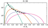 |
Fig. C.1. Solid coloured lines show examples of model radial profiles across a cylindrical jet of radius Rj of momentum flux density S(R) (defined by Eq. C.1) normalised by the mean value ⟨ S⟩ (Eq. C.2) for p = 2 and different values of q (corresponding to Rpeak/Rj = 1/10, 1/5, 1/3, 1/2). The thick dashed line shows the enhancement factor fS = Speak/⟨ S⟩ (Eq. C.3) as function of Rpeak/Rj. |
All Tables
All Figures
|
Fig. 1. Logarithms, f = log10(F), of volume distributions, F(μ) = dF/dμ, over the argument μ = log10(u/uB, 0), with u the energy density: of magnetic fields, uB = B2/8π (left panel), and of the plasma, upl = ⟨γ⟩nmc2 (right panel). Functions f(μ) were averaged over the duration of each simulation. |
| In the text | |
|
Fig. 2. Maps of log10(u/uB, 0)(x, y) for magnetic energy density, uB = B2/8π (upper panels), and plasma energy density, upl = ⟨γ⟩nmc2 (middle panels), for relaxed monster plasmoids at the end of each simulation. In the lower panels, we compare 1D energy density profiles of (u/uB, 0)(x, y0) measured along the strip indicated in the above maps by the dashed grey lines. A common colour scale for all maps is referenced along the left axes in the lower panels. Here, we present the effect of a guide field for σ0 = 10 and L/ρ0 = 1800. From the left, the columns show simulations: (1) L1800_σ10, (2) L1800_σ10_Bg05, and (3) L1800_σ10_Bg1. |
| In the text | |
|
Fig. 3. Profiles of magnetic (green lines) and plasma (red lines) energy densities across (i.e. along the y coordinate) relaxed monster plasmoids. Panels from the left compare: (1) different sizes, L/ρ0, of simulation domain (2D with σ0 = 10, Bz = 0); (2) different magnetisations, σ0 (2D with L/ρ0 = 1800, Bz = 0); (3) 3D and 2D domains (with L/ρ0 = 900, σ0 = 10, Bz = 0); (4) different guide field strengths, Bg/B0 (2D with σ0 = 10, L/ρ0 = 1800). |
| In the text | |
|
Fig. 4. Same as Figure 2, but for plasmoid mergers that maximise the plasma energy density, upl, for the same set of simulations: (1) L1800_σ10, (2) L1800_σ10_Bg05, and (3) L1800_σ10_Bg1. |
| In the text | |
|
Fig. 5. Same as Figure 1, but for the open-boundary simulations with synchrotron cooling first presented in Ortuño-Macías & Nalewajko (2020). The black dashed lines indicate power laws of index −5/3. |
| In the text | |
|
Fig. 6. Proposed lateral structure (not to scale) of a relativistic jet differentiated due to poloidal field bunching. The ‘bunched spine’ zone is introduced as the region maximizing the jet energy flux density. The introduction of plasmoids from reconnection layers created due to CDI in the jet core allow the energy density enhancement factors of the plasmoids and of the bunched jet spine to multiply. |
| In the text | |
|
Fig. C.1. Solid coloured lines show examples of model radial profiles across a cylindrical jet of radius Rj of momentum flux density S(R) (defined by Eq. C.1) normalised by the mean value ⟨ S⟩ (Eq. C.2) for p = 2 and different values of q (corresponding to Rpeak/Rj = 1/10, 1/5, 1/3, 1/2). The thick dashed line shows the enhancement factor fS = Speak/⟨ S⟩ (Eq. C.3) as function of Rpeak/Rj. |
| In the text | |
Current usage metrics show cumulative count of Article Views (full-text article views including HTML views, PDF and ePub downloads, according to the available data) and Abstracts Views on Vision4Press platform.
Data correspond to usage on the plateform after 2015. The current usage metrics is available 48-96 hours after online publication and is updated daily on week days.
Initial download of the metrics may take a while.