| Issue |
A&A
Volume 696, April 2025
|
|
|---|---|---|
| Article Number | A141 | |
| Number of page(s) | 32 | |
| Section | Stellar atmospheres | |
| DOI | https://doi.org/10.1051/0004-6361/202346391 | |
| Published online | 17 April 2025 | |
FENRIR: A statistical model of stellar variability
I. A physics-based, fast Gaussian process model to represent stellar activity and perform statistical Doppler imaging
1
Aix Marseille Université, CNRS, CNES, LAM,
Marseille,
France
2
Observatoire Astronomique de l’Université de Genève,
51 Chemin de Pegasi,
1290
Versoix,
Switzerland
★ Corresponding authors; This email address is being protected from spambots. You need JavaScript enabled to view it.
; This email address is being protected from spambots. You need JavaScript enabled to view it.
Received:
13
March
2023
Accepted:
26
January
2025
Abstract
Context. Stellar surfaces exhibit magnetic activity, which manifests in photometric and spectroscopic observations as a stochastic process. Precisely understanding its statistical structure is crucial for distinguishing stellar variability from signals of potential exoplanets. Furthermore, it could provide insights into the star itself.
Aims. Photometric and spectroscopic observations – including radial velocities (RVs) – can be described by their joint statistical distribution as a function of model parameters, also called the likelihood function. We aim to derive a likelihood function from a quantitative physical model.
Methods. We modeled stellar activity as a stochastic process and analytically derived its Gaussian process (GP) approximation in two variants: a fully physics-based joint model of RVs and photometry, and a model that retains the physical motivation while incorporating data-driven assumptions, applicable to any combination of photometric and spectroscopic measurements. The GP kernels are implemented in a public Python package using the S+LEAF framework, ensuring that likelihood evaluations scale linearly with data size.
Results. We applied our method to solar observations, HARPS-N spectroscopy and SORCE photometry. We show that the FENRIR GPs significantly outperform existing ones in terms of cross-validation. We give a proof of concept of “statistical Doppler imaging,” constraining the average properties of stellar spots and faculae even when they are too small to be individually resolved. Using only the statistical properties of RVs and photometry, we estimate the solar sky-projected obliquity with a precision of ~5°, Finally, we discuss the limitations of our model and exhibit non-Gaussianity in solar HARPS-N RVs.
Key words: methods: statistical / techniques: photometric / techniques: radial velocities / Sun: activity / sunspots / planets and satellites: detection
Both authors contributed equally to this work.
© The Authors 2025
 Open Access article, published by EDP Sciences, under the terms of the Creative Commons Attribution License (https://creativecommons.org/licenses/by/4.0), which permits unrestricted use, distribution, and reproduction in any medium, provided the original work is properly cited.
This article is published in open access under the Subscribe to Open model. This email address is being protected from spambots. You need JavaScript enabled to view it. to support open access publication.
1 Introduction
Stellar surfaces exhibit a variety of physical processes occurring on different timescales, including acoustic oscillations, granulation, super-granulation, and magnetic activity (Rincon & Rieutord 2018; Cegla 2019; Meunier 2023). These phenomena have signatures in photometric and spectroscopic data, which can be considered either as signal or noise depending on the scientific objective. In the context of Doppler imaging, the magnetic activity signature is the signal of interest. As the star rotates, the inhomogeneities in the stellar surface create spectral line shape changes. From high-resolution spectra taken at different stellar rotational phases, the goal is to infer a specific intensity map of the stellar surface (Deutsch 1958; Khokhlova 1976; Goncharskii et al. 1977, Goncharskii et al. 1982; Vogt & Penrod 1983; Vogt et al. 1987; Donati et al. 1997; Luger et al. 2021a). In contrast, the complex variability induced by stellar processes poses a significant challenge to exoplanet detection and characterization (Mayor et al. 2014; Sulis et al. 2020; Crass et al. 2021; Hara & Ford 2023). The goal of this series of articles is to provide a detailed, physics-based description of stellar variability signals seen as stochastic processes, useful both to model them as a noise and to gain insight on the star. In this study, we focus on stellar magnetic activity, hereafter referred to as stellar activity.
Stellar activity refers to the ensemble of processes occurring on and above a star’s surface, driven primarily by magnetic fields in the outer stellar layers. In particular, transient features might appear on the surface of stars: starspots (regions of reduced surface temperature caused by strong magnetic fields), or bright regions called faculae (see Fig. 1, and Schrijver 2002; Strassmeier 2009). Spots and faculae create an imbalance of flux on the star. Furthermore, they locally inhibit the convective motion of the gas on the stellar surface (Dravins et al. 1981). Overall, they create complex patterns in photometric and spectroscopic data (Saar & Donahue 1997; Desort et al. 2007; Meunier et al. 2010b; Boisse et al. 2012; Dumusque et al. 2014; Borgniet et al. 2015; Meunier et al. 2019; Meunier & Lagrange 2019a,b). Be they considered as signal or noise, activity-induced signals must be modeled precisely. This can be done by choosing a probability distribution of the data knowing the parameters of the signal of interest, or likelihood function.
In the context of Doppler imaging, the data consist in a time series of spectra taken over one or several rotation periods, possibly with contemporaneous photometry. The likelihood parameters describe the specific intensity map of the stellar surface, allowing one to recover the position of dark and bright magnetic regions. The parameters can be chosen as intensities on a grid covering the visible hemisphere Khokhlova (1976); Piskunov & Rice (1993) or coefficients of spherical harmonics (Luger et al. 2021a). Regardless of the parametrization, the stellar surface properties are usually retrieved by searching the parameters that fit the data best, or equivalently, that maximize the likelihood. Since several intensity maps can fit the data, it is common practice to include a regularization scheme (e.g., Goncharskii et al. 1977, Goncharskii et al. 1982; Donati et al. 1997; Petit et al. 2015). This is equivalent to choosing a prior, and maximizing the posterior distribution of the parameters describing the stellar surface. Alternatively, this posterior probability can be computed directly, which has the advantage of giving uncertainties on the reconstructed map Luger et al. (2021b,a).
In the context of exoplanets, the data are spectroscopic or photometric time series, possibly both. Most stars observed do not rotate sufficiently fast, nor do they exhibit sufficient levels of activity to resolve the stellar surface at a given time. Likelihood parameters related to stellar activity include stellar rotation period and the average lifetime of magnetic regions. The likelihood is almost always assumed to be Gaussian (Aigrain et al. 2012; Haywood et al. 2014; Rajpaul et al. 2015; Foreman-Mackey et al. 2017; Gilbertson et al. 2020; Jones et al. 2022; Hara & Ford 2023; Tran et al. 2023). Its exact parametric form has an impact on the inferred properties of the star and of the putative planets (e.g., Ahrer et al. 2021; Suárez Mascareño et al. 2021). In existing works, the likelihood parameters are not clearly related to physical quantities.
Our aim is to build a likelihood of photometric and/or spectroscopic time series given the average properties of stellar activity – the exoplanet case – which is rooted in a physical model. Conceptually, our solution consists of establishing an analytical link between the likelihood and prior used in Doppler imaging, and the one used in exoplanets. Our framework serves two purposes. First, one can expect that physics-based models disentangle more efficiently the signals due to stellar activity and planets. Second, a physics-based statistical model offers a new way to perform Doppler imaging. Indeed, Doppler imaging is possible only if several conditions are met (e.g., Rice & Strassmeier 2000; Kochukhov 2016): stellar regions must have a sufficient area and contrast to be resolved, the star needs to rotate sufficiently fast in order to see spots move across spectral lines, and the spots must be sufficiently stable during the observation time. However, one can envision that even if one of the conditions is not met and the regions cannot be resolved individually, it might be possible to perform “statistical Doppler imaging”; that is, to retrieve average properties of the stellar surface (stellar inclination, average latitude of spots, etc.).
The article is organized as follows. In Section 2, we present our general statistical formalism to transfer a physical model of the effect of magnetic regions to a likelihood function. We specify the model in Section 3 in two ways. First, we give a fully physics-based model for radial velocity (RV) and photometric observations. Second, we build a general model class that still retains the physical motivation but is more agnostic to the exact assumptions, and that can be applied to any combination of observables of a star (photometry, RV, spectroscopy, etc.). In Section 4, we describe the practical computation of the kernels. In Section 5, we apply our formalism to the analysis of HARPS-N and SORCE observations of the Sun. We compare the performances of the new and existing kernels, and we discuss the ability of physics-based FENRIR kernels to retrieve stellar inclinations as well as average properties of the magnetic regions. In Section 6, we discuss the limitations of our model. In particular, we highlight the presence of non-Gaussianity in RV observations of the Sun. We conclude in Section 7. We provide a public implementation of the FENRIR GPs with tutorial notebooks1.
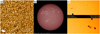 |
Fig. 1 (a) Inouye Solar Wave Front Correction (WFC) image, captured on Jan. 28, 2020, at 789 nm. The granulated structures around the spot are due to convection: hot plasma moves upward at the center of granules, cools down, and goes downwards between granules (darker intergranular regions). The contribution of brighter intra-granular regions exceeds that of intergranular ones, creating a so-called convective blueshift on observed spectra. Credit: NSO/AURA/NSF. (b) SDO observation of the Sun at wavelength 1700 Å. The bright regions are called faculae, and the dark regions are called spots. Both faculae and spots inhibit the upward convective motion of the gas (Dravins et al. 1981). Faculae cover more area than spots, but have a smaller temperature contrast with the quiet surface. The latitude, number, and lifetime of the spots varies along stellar magnetic cycles, on the timescale of a few years (11 years for the Sun). Courtesy of NASA/SDO and the AIA, EVE, and HMI science teams. (c) Group of sunspots observed at two different dates, top: January 6, 2012, bottom: January 8, 2012. Courtesy of NASA/SDO. |
2 Statistical framework
2.1 Gaussian likelihoods: Existing approaches
We shall first briefly present how likelihoods are usually defined for exoplanet searches, with the Gaussian process (GP) framework. In general, the data consist of photometric observations, or RVs and spectral indicators, possibly both (see e.g., Hara & Ford 2023). For the sake of clarity, we first consider the case where there is only one type of observations. For example, if we have photometric observations, Y = (y(tn))n=1..N where y(tn) is the photometric observation at time tn. The likelihood is chosen as a Gaussian distribution, which is fully characterized by its mean f (η) and covariance matrix V(η), and has the form
![Mathematical equation: $p(Y\mid \eta ) = {{\exp \left[ { - {1 \over 2}{{(Y - f(\eta ))}^T}{\bf{V}}{{(\eta )}^{ - 1}}(Y - f(\eta ))} \right]} \over {\sqrt {{{(2\pi )}^N}\left| {{\bf{V}}(\eta )} \right|} }}.$](/articles/aa/full_html/2025/04/aa46391-23/aa46391-23-eq1.png) (1)
(1)
 denotes the determinant of matrix V(η) and the subscript denotes matrix transposition. To simplify the notations but without loss of generality, we assume that η are the parameters of stellar activity. One can easily change Eq. (1) to account for planets, offsets etc. by adding another deterministic term in the mean (see Hara & Ford 2023), f (η) must be replaced by f (η) + h(θ) where h(θ) represents the expected signal of the planets, offsets, trends, depending on parameters θ. To add the observational uncertainties, denoting by Σ the diagonal matrix whose entries are
  , where σi is the error on observation i. The covariance V(η) must be replaced by V(η) + ς.
The value of V at row m and column n quantifies the similarity of the noise values at times tm and tn . Typically, the stellar noise is assumed to be stationary and is defined with a kernel function,
 (2)
(2)
For instance, the so-called quasi-periodic kernel (Aigrain et al. 2012; Haywood et al. 2014) is defined by a vector η of four parameters (η1, η2, ηз, η4),
![Mathematical equation: ${k^{{\rm{QP}}}}\left( {\left| {{t_m} - {t_n}} \right|,\eta } \right) = \eta _1^2\exp \left[ { - {{{{\left( {{t_m} - {t_n}} \right)}^2}} \over {2\eta _2^2}} - {{2{{\sin }^2}{{\pi \left( {{t_m} - {t_n}} \right)} \over {{\eta _3}}}} \over {\eta _4^2}}} \right].$](/articles/aa/full_html/2025/04/aa46391-23/aa46391-23-eq5.png) (3)
(3)
This kernel qualitatively expresses that the surface of the star remains similar to itself, though not identical, after one stellar rotation. The parameters η2 and η3 can be interpreted as the average lifetime of magnetic regions and the stellar rotation period, respectively. However, none of the parameters are clearly related to a physical model.
When several time series are available, it has been shown to be much better practice to analyze them jointly than separately (Rajpaul et al. 2015; Eastman et al. 2019; Hara & Ford 2023; Yu et al. 2024). We call these different observation types “channels”, and we suppose that we have q channels, not necessarily sampled at the same epochs. For instance, we might have observations through q = 2 channels: photometry and RVs. Channel i has Ni observations and is sampled at times  ,n = 1..Ni, and we call the vector of all observations Y =
 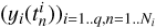 . The likelihood of data Y can still be described by Eq. (1). In existing works, the mean is always assumed to be zero. The covariance matrix can be seen as a block matrix, each i, j block gives the covariance between channels i and j. It is characterized by the kernels
 (4)
(4)
Multichannel Gaussian models are often chosen such that each channel is a linear combination of a GP and its derivatives (Rajpaul et al. 2015; Gilbertson et al. 2020; Jones et al. 2022; Delisle et al. 2022). This comes down to choosing a certain parametric form for Eq. (4) (see Gilbertson et al. 2020, Eqs. (8) and (9)). Eq. (4) can also be used when the channels are fluxes at different wavelengths, thus encompasses transit spectroscopy (Gibson et al. 2012; Gordon et al. 2020; Fortune et al. 2024), as well as the statistical Doppler imaging problem introduced above. In summary, both in the single and multi channel case, the data can always be represented as a single vector, and its Gaussian likelihood is fully characterized by mean and covariance functions.
2.2 FENRIR kernels
At the end of our derivations in Section 4, we establish that for any data, Y, consisting of several time series, FENRIR GPs have a kernel associated with channels i and j is of the form
 (5)
(5)
where kW(τ; η) is the part of the kernel corresponding to the intrinsic evolution of spot and faculae properties, and  is the periodic part of the kernel, corresponding to the changing viewing geometry as the star rotates. The kernel kλ(τ; η) accounts for the magnetic cycle, and its amplitude changes depending on the two channels i, j through a multiplicative coefficient, ai,j(η).
Eq. (5) has a similar structure to Eq. (3): a decaying function times a periodic one, but in FENRIR models the exact parametric form of the kernel and the hyperparameters are linked to a physical model.
2.3 Finite energy nonlinear impulse response (FENRIR)
Our aim is to describe the statistical distribution of multichannel data, Y, knowing the stellar parameters η, p(Y | η). The first step of our reasoning is to build a physically motivated random process, without assuming it Gaussian. Below, we describe how to generate a sample from p(Y | η).
The first step consists of generating a collection of times of arrival of spots and faculae, (tk)k= −∞..+∞. The appearance rate and the properties of spots and faculae vary with the magnetic cycles of stars on the timescales of several years (~ 11 years on the Sun) (Martinez Pillet et al. 1993; Borgniet et al. 2015). We refer to transient magnetic regions (spots, faculae, or groups of those) as stellar “features”. Features appear at times drawn from a Poisson process, just like the times of arrival of photons counted on a detector. Poisson processes are characterized by the average number of events per time unit, which might vary with time, λ(t).
When a stellar feature appears at time tk, its properties γ(tk) are drawn from a distribution p(γ | η, tk). This simply means that the properties of the feature depend both on the properties of the star, η, and the time at which it appears tk . When a stellar feature appears at time tk and has parameters γ(tk) it is assumed to have an effect gi(t − tk, γ(tk)) on channel i. For the observation geometry represented in Fig. 2, in Fig. 3 we show the effect of a point-wise dark spot with constant latitude, size and contrast on RVs and photometry.
We use the notation X ~ p(x) to indicate that the random variable X is drawn from the probability distribution p(x). Our model can be simply expressed with three equations.
 (6)
(6)
 (7)
(7)
 (8)
(8)
where
λ(t) is called the Poisson rate.
p(γ | t, η) is called the distribution of feature parameters.
ɡi(t, γ) is called the impulse response on channel i.
FENRIR models are filtered Poisson processes (e.g., Lefebvre & Bensalma 2015), where we make the additional assumption that the impulse response has always a finite energy.
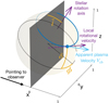 |
Fig. 2 Viewing geometry: a stellar feature represented by the dark blue point moves as the star rotates and is visible only a fraction of the time. It modifies the local emission, and velocity of the plasma, which appears to move outwards because of its convective motion. We parametrize the position of the feature with the angle between the sky plane and rotation axis, |


2.4 Likelihood of FENRIR models
Regardless of the exact choice of parametrization of our model, given data Y we could try to determine exactly which features affect the dataset. We now need to search their number K, find their times of appearance (tk)k =1,..,K, and estimate their parameters (γ(tk))k=1,..,K. We could search feature parameters with maximum posterior probability, or equivalently minimum – log posterior probability. Using the notation (tk) = (tk)k =1,..,K for simplicity, we would solve
 (9)
(9)
This is similar to the approach taken in Dumusque (2014), which fits a spot model generated with SOAP 2.0 simulations (Dumusque et al. 2014) onto RVs and spectral indicators.
In Eq. (9), the first term and second term in the sum have a counterpart in the Doppler imaging literature. Assuming a Gaussian likelihood, they correspond respectively to the χ2 and the regularization term (maximum entropy or Tikhonov, e.g., Goncharskii et al. 1977, 1982; Petit et al. 2015). Usually, in Doppler imaging the fitted parameters do not describe the individual active region, but the local line depth on the stellar surface (Piskunov & Rice 1993; Luger et al. 2021a). Still, the goal is to retrieve the state of the stellar surface with a certain regularization scheme.
However, for slow rotating stars, often targeted to search for exoplanets (Lovis & Fischer 2010), it is impractical to fit the properties of individual magnetic regions. The approach taken here is to compute p(Y | η). We need to marginalize the distribution p(Y | (tk), (γk), η) over (tk), (γk). We found that the marginalized likelihood is impractical to compute analytically. However, we can approximate it by a Gaussian likelihood.
To obtain a Gaussian likelihood in the form of Eq. (1), we computed the mean and covariance of the FENRIR process presented in Section 2.3. The calculation is presented in Appendix A.1. The mean of the FENRIR process for channel i evaluated at time  is given by
 (10)
(10)
and the covariance between the channels i and j evaluated at times  , respectively, is
 (11)
(11)
Eqs. (10), and (11) define unambiguously a Gaussian likelihood.
The Gaussian representation (1) is only an approximation of the likelihood of a FENRIR process. In particular, the higher- order cumulants of the FENRIR processes are usually non-zero. This aspect is further discussed in Section 6.2.
Eq. (11) is not yet identical to the FENRIR kernel in Eq. (5). To obtain this latter expression, as well as guaranteeing a O(N) cost of likelihood evaluation, we need further hypotheses on the impulse responses ɡj(t, γ), the statistical distribution of γ, p(γ | t, η), and the Poisson rate λ(t), which we now turn to.
3 Physical and data-driven models
FENRIR likelihoods come in two flavors: physics-based and data-driven. In the first case, we start from quantitative physical arguments to determine the impulse responses, distribution of feature parameters and Poisson rate (see Sections 3.1–3.3). In the data-driven case, we search those in a wide class of functions, not explicitly tied to physical parameters (Section 3.4).
3.1 Impulse response
Spots and faculae affect the photometry and spectroscopy in several ways. While spots are darker than their surroundings, faculae are brighter. Consequently, as they pass accross the visible hemisphere of the star, they have an a photometric effect. Secondly, because they break the flux imbalance of the approaching and receding limb of the star, they have a Doppler signature. Finally, their magnetic field inhibits the convection motion of the plasma in the stellar photosphere. The hot plasma has an upward motion, it cools down and moves back towards the center of the star. Because the plasma moving outwards is hotter, it represents a higher fraction of the total flux resulting in a global blueshift of the stellar light. In spots and faculae, the magnetic field tends to globally slow this motion, resulting in the so-called inhibition of the convective blueshift (Dravins et al. 1981; Meunier et al. 2010a; Dumusque et al. 2014).
To derive analytical expressions of the impulse responses, we made simplifying assumptions, whose validity is discussed in Section 6.1. First, we assume that the measured RV are the sum of the local RVs of the star weighted by their flux. Second, we assume that active regions are point-wise. We denote with ϕ and δ the latitude and longitude of the magnetic region on the stellar surface. We assume that the stellar rotation axis is well defined, and denote with  its angle respective to the sky plane (see Fig. 2). Our formalism can account for differential rotation. However, for the sake of simplicity, we assume a solid body rotation,
 (12)
(12)
In Appendix B, we show that with our assumptions, the photometric and inhibition of convective blueshift effects in RV, ɡph and ɡcb , and the effect on photometry h are
 (13)
(13)
 (14)
(14)
 (15)
(15)
where R⋆ is the stellar radius, 1vis(t) equals one when the feature is in the visible hemisphere, and 0 otherwise, ΔF is the flux difference of the magnetic region with the quiet surface flux, and Δ Vcb is the difference between the mean velocity of the flow of the quiet surface and of the magnetic region. The function W(t) models the variation in the amplitude of the magnetic region as a function of time and is parametrized by a time scale of the appearance of spots ρ. By convention, we consider that W(t) attains its maximum (maximal area of the feature) at t = 0 for this impulse response. The quantity µ is the ratio between the surface of the magnetic region projected onto the sky and its intrinsic surface,
 (16)
(16)
We have µ = cos ψ, where ψ is the angle between the line of sight and the normal to the magnetic region. As such, it is the quantity classically used to express limb-darkening laws. To simplify the notation, we use µ instead of  .
.
The central part of the Sun appears brighter than its edges, a phenomenon known as limb-darkening, also present in other stars. Furthermore, faculae and their counterpart in the chromosphere, plages, have a limb-brightening effect which counteracts the limb-darkening behavior of the flux (Frazier 1971; Unruh et al. 1999; Meunier et al. 2010a). The functions lph, lcb, and lf in Eqs. (13)–(15) are limb-darkening/brightening laws, which are functions of µ, and which we assume to be polynomials of the form:
 (17)
(17)
In Fig. 3, we show ɡph, ɡcb and h as a function of time for different spot latitudes and stellar inclination, assuming solidbody rotation and constant limb darkening. In Fig. 4, we illustrate the effect on RV of different limb-darkening laws. The limbdarkening effect tends to smooth the effect of a spot, and shift the maximal effect towards the longitude of the observer. The term Wρ(t) captures the increase and decrease in intensity as spots and faculae grow and vanish (see Fig. 5).
We assume that the effect of a given magnetic region in RV is a weighted sum of the photometric and convective blueshift inhibition effect, and that both effects obey a common limbdarkening law. Due to the degeneracies between the amplitude coefficients, we adopt the following parametrization for the effect of a spot or facula,
 (18)
(18)
 (19)
(19)
with γ = (δ, ϕ0, ρ, σphot, σrv-cb, σrv-phot, ω,  , a) and where ϕ(t) is given in Eq. (12), and σrv-cb, σrv-phot and σphot are free parameters controlling the amplitude of the respective contributions of the RV inhibition of convective blueshift, RV photometric effect, and flux effect in the photometric time series.
In the FENRIR model, it is supposed that stellar features appear potentially with a variable rate, but independently of each other. However, magnetic regions might appear in certain configurations. On the Sun, spots typically appear on longitudes shifted by 180° (Korhonen et al. 2001; Berdyugina & Usoskin 2003; Borgniet et al. 2015), and there is evidence that this behavior has effects in the Sun HARPS-N RV measurements (Hara et al. 2022). To take this into account, we consider the impulse response g as the effect of two groups of spots shifted by 180°. Overall, using the notations of Eqs. (18) and (19), the expression for the impulse response on RV and flux are
 (20)
(20)
 (21)
(21)
with γ = (δ, ϕ0, ρ, σphot, σrv-cb, σrv-phot, α180, ω,  , a). Eqs. (20) and (21) can be used to model the effect of spots or faculae, or their combined effect. We can further extend this idea to groups of four spots or faculae, two symmetric about the equator and two shifted by 180° (see Section 5).
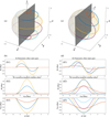 |
Fig. 3 In (a) and (c), colored lines represent the path of dark spots as the star rotates at different latitudes. In (a), the rotation axis in the plane of the sky, in (c) the rotation axis is tilted by 0.5 rad towards the observer with respect to the sky plane. (b1)/(d1): effect on RV of the imbalance break between the approaching an receding limb (ɡph in Eq. (13)), (b2)/(d2): RV convective blueshift inhibition effect on RV (ɡcb in Eq. (14)), (b3)/(d3): effect on photometry of the stellar surface darkening (h in Eq. (15)). |
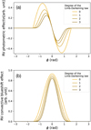 |
Fig. 4 Different RV effects of an equatorial dark spot due to the photometric effect (a) and inhibition of the convective blueshift (b), with limb-darkening laws of different degrees (simply l(µ) = µ,µ2,µ3). With the notations of Eq. (17), in increasingly darker yellow we take d = 0,1,2,3 and for j < d, aj = 0. |
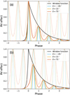 |
Fig. 5 RV convective blueshift inhibition on the RVs as a function of the rotation phase with a rising and decaying amplitude with a star inclined as in Fig. 3d. Black line: window function consisting of two exponentials, thin lines: effect of a spot without amplitude variation, bold lines: effect of the spot with varying amplitude. Colors correspond to the effect of spots at different latitudes (color code is the same as Fig. 3d). In (a) the maximum amplitude of the spot is attained on the visible hemisphere at the longitude of the observer (ϕ0 = 0), and in (b) the maximum amplitude is attained when the spot is 180° away from the observer. The window is chosen to reproduce the fact that, on the Sun, spots appear 10-11 times faster than they vanish (Howard 1992; Javaraiah 2011). |
3.2 Distribution of spots and faculae parameters
In the FENRIR formalism of, each time a feature appears, its parameters γ must be drawn from the distribution of features (Eq. (7)). The parameters of the individual features γ are δ the latitude, ϕ0 the longitude at which the feature reaches its maximal area, ρ the lifetime, σphot , σrv-cb , σrv-phot the amplitudes in photometry and in RV, α180 the amplitude of the opposite magnetic region, ω the angular velocity (or the rotation period P),  the stellar inclination, a the limb-darkening coefficients. The parameters ρ, σphot, σrv-cb, σrv-phot, α180, ω,
  , a are supposed to be identical for all magnetic regions and are included in the population parameters η. The only parameters drawn randomly from the distribution of feature parameters are (δ, ϕ0).
In the present work, we assume that the longitude at which the feature reaches its maximal area, ϕ0 , is uniformly distributed on [0,2π]. The latitude is drawn from two Gaussian distributions, symmetrical about the stellar equator, of means ±µδ and standard deviation σδ. Overall, we have population parameters η = (µδ, σδ, ρ, σphot, σrv-cb, σrv-phot, α180, ω,  , a).
, a).
The assumption that the parameters σrv-cb , σrv-phot, σphot and ρ are the same for all magnetic regions might seem simplistic. However this is not a huge loss of generality. As explained in Appendix C, σrv-cb , σrv-phot , σphot and ρ can be interpreted as the average properties of magnetic regions. Finally, we assume that p(γ|η, t) = p(γ|η), the distribution is independent of time. The model still accounts for the higher rate of apparition of magnetic regions at maximum activity.
3.3 Poisson rate
To specify the FENRIR model, we must choose the rate at which features appear on the star (λ(t) in Eq. (6)). This expresses the fact that the number of magnetic region varies with the magnetic cycle. In Fig. 6 we represent a RV time series simulated with a FENRIR process, such that there are ~50 visible spot groups per day, as observed on the Sun. The effect of inhibition of the convective blueshift is always positive, and as a consequence, a higher appearance rate of magnetic regions translates to a systematic RV effect.
In the present work, we assume that the function λ(t) is itself a stochastic process with a known mean function and covariance, similarly to the approach taken in Camacho et al. (2023). As we shall see in Section 4, this allows for great flexibility as well as a computationally efficient evaluation of the likelihood.
3.4 Formal assumptions for the physics-based and data-driven models
In Sections 3.1–3.3, we specified the key ingredients of the FENRIR model (Eqs. (6)–(8)). Their validity is discussed in Section 6.1. Our hypotheses can be summarized by the following formal assumptions.
-
The impulse response on channel number i, ɡi(t, γ), is represented as a product of a time window and a periodic part, each with their own variables. Denoting by γ = (γw, γper, ϕ0),
 (22)
(22)In the computations, Pi is assumed to be in the form of a Fourier series
 (23)
(23)where ik(γper) are the k-th Fourier coefficient of Pi(t, γper). In the case where the signal is real-valued, as is the case here, we have
 denotes the complex conjugate of z. For the sake of simplicity, the window function is the same in all the different channels.
Fig. 5 gives an example of this representation. The black line represents W(t, γW) for a certain value of γW, the thin and thick colored lines represent Pi(t, γper, ϕ0) and ɡi(t, γ), respectively, for three values of γper. Figs. 5a and b represent these quantities for two values of ϕ0.
The phase ϕ0 is distributed uniformly on [0,2π]. That is, the longitude at which the magnetic regions attain their maximal size is random on [0,2π].
-
The parameters of the window and of the periodic parts are supposed to be statistically independent,
 (24)
(24)In the context of stellar activity, it means that the evolution of the size of a magnetic region is independent of its longitude and latitude.
We assume that the properties of the distribution of feature parameters are independent of time, p(γ|η, t) = p(γ|η).
We assume that λ(t) is a stationary random process with expectation µλ(η), and covariance function kλ(τ; η).
The variation timescale in λ(t) is much greater than 2π/ω (defined in Eq. (23)): the magnetic cycle has a much longer timescale than the stellar rotation period.
In the physics-based setting, we obtained analytical expressions for each of mathematical expressions appearing in assumptions 1–6. The data-driven kernel consists in considering that the real and imaginary parts of the Fourier coefficients in Eq. (23) are the parameters η of our model. As shown in Section 4.3, if we do so, there is no need to specify the distribution of feature parameters.
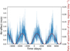 |
Fig. 6 Simulated RV as a function of time when the RV effect is due to a combination of inhibition of convective blueshift and a RV photometric effect. The average lifetime of the magnetic regions is 15 days. The rate varies as a A/2(1 + cos 2πt/Pmaɡc) where Pmaɡc = 11 years and A is such that there are on average 50 spots visible each day. |
4 The physics-based and data-driven kernels
4.1 Computations
From assumptions 1–6 in Section 3.4, in Appendix C we show that the covariance between a measurement taken in channel i at t and channel j at t + τ is of the form of Eq. (5), which is reproduced below for convenience,

such that
 (25)
(25)
 (26)
(26)
 (27)
(27)
where µi(η) = Eγ(i0(γ)), µj(η) = Eγ(j0(γ)), the mathematical expectancy of i0 and j0 defined in Eq. (23). The kernel, kλ(τ; η), is the covariance λ(t). It accounts for the magnetic cycle, and its amplitude changes depending on the two channels i, j through a multiplicative coefficient, ai, j . The fact that this covariance term is additive is a simplification due to assumption 6. If the time-scale of stellar rotation and magnetic cycle were closer, the expression of the FENRIR kernel would be more complex (see Appendix C.6). The periodic part of the kernel can be expressed in a Fourier series,
 (28)
(28)
where
 (29)
(29)
d, ik and jk being respectively the number of harmonics, and the Fourier coefficients of the impulse responses in channels i and j (see Eq. (23)).
In Appendix C, we present a method to evaluate the likelihood with a cost ∝ NrW(2d + 1) where N is the total number of data points, rw a coefficient linked to the window (typically one to three), and d is the number of harmonics in the Fourier expansion of the periodic part. This computational scheme applies both to the physics-based and data-driven models, we now highlight their specificities.
4.2 The physics-based kernels
In the case of the physical model, the kernel  is fully specified by the choices made in Section 3. However, for a specific choice of the distribution of spots latitudes and longitudes, the integral in Eq. (29) may not have an analytical expression. This can be circumvented in two ways. The first option consists in considering that the impulse response has always the same parameters, and that the average group of magnetic regions that it describes represents the average effect of magnetic regions. The second option is, for a given value of the hyperparameters η, we compute this integral numerically by discretizing the feature parameters γper. To improve performances, we precompute the integrals on a grid of values of hyperparameters, so that, when we need to evaluate the likelihood for a given value of η, we simply interpolate the integral values computed on the grid (the exact procedure is slightly more elaborate, see Appendix C).
In Section 3, we did not specify our choice for the evolution of the size of stellar spots and faculae, W(t). In Section 5, we use Matérn 1/2 or Matérn 3/2 kernels corresponding, respectively, to assuming that W(t) is a one-sided exponential or symmetric exponential (see Table C.1). Finally, for the kernel representing the magnetic cycle, kλ , we used a Matérn kernel.
4.3 The data-driven MultiFourierKernel
The physics-based model is specified only for RV and photometry. Furthermore, the physical assumptions on the impulse response and distribution of feature parameters might be faulty, and we could want to be more agnostic to them. Interestingly, for any choice of spectroscopic indicator and photometric channels, all the possible FENRIR kernels with assumptions 1–6 can be written as in Eq. (5) where the periodic part of the kernel is what we call a MultiFourierKernel,
 (30)
(30)
where ak(η) = (ak;i,j(η))i,j =1..q and bk(η) = (bk;i,j(η))i,j =1..q are q × q matrices defined as
 (31)
(31)
 (32)
(32)
where η = (αk, βk)k=0..d, and matrices αk, βk have a form
 (33)
(33)
 (34)
(34)
For real-valued data, they satisfy α−k = αk and β−k = −βk. In particular, for k = 0, β0 = 0.
If we were to choose the expression of the Fourier coefficients ik(γ) and the distribution p(γ | η) as generally as possible, we would not have a class of kernels more general than simply choosing as hyperparameters η the coefficients of matrices αk and βk, k = 0,…, d.
Here we have q observational channels. If we choose η = (αk, βk)k=0..d, everything happens as if there were q FENRIR processes indexed by l = 1..q, statistically independent and with the same rate, which have a fixed impulse response of the form Eq. (23), and which we call modes. In the context of stellar activity, this means that everything happens as if there were at most q equivalent spots, always with exactly the same parameters, appearing independently of each other. The matrices α and β define the real and imaginary parts of these “equivalent spots”/modes up to a factor (see Eq. (35)).
For k > 1, αk and βk matrices respectively have q(q + 1) and q(q − 1) free coefficients, so in total the model has q2 real-valued coefficients per harmonic. For k = 0 there are only q(q + 1)/2 real coefficients. There are d harmonics. In total, we have at most dq2 + q(q + 1)/2 free coefficients in the model. However, we can make an assumption on the rank of the matrices αk and βk, which reduces the number of free coefficients. In the following sections, we refer to the number of columns of αk and βk that are non-zero as the number of modes, and denote it by m. Overall, the MultiFourierKernel is defined by the number of modes m and the maximum harmonic order d (see Eq. (23)).
For instance, if we assume a single mode, only the coefficients of the first column of are non zero. It comes down to assuming that it is always the same equivalent spot that appears randomly. Assuming that d = 3 harmonics are used, everything happens as if there was a single type of spot appearing randomly, of impulse response on channel j,
 (35)
(35)
with  and
and  for k = 1,2,3.
It might seem surprising that in the data-driven version of FENRIR, the number of equivalent spots depends on the number of channels. This can be understood intuitively in the three- channel case outlined above, by considering that three types of magnetic regions might appear, each affecting only a certain channel. For example, spots of type one are only visible in RV, spots of type two in photometry, etc. To describe this situation, we need three independent templates. This case, although not physically motivated, shows that q templates might be needed to describe q channels. The fact that more than q templates do not introduce more expressivity of the kernels comes from degeneracies of the approximation of FENRIR processes by GPs. We refer the reader to Appendix C.7 for more details.
5 Analysis of HARPS-N solar RVs and SORCE Total Solar Irradiance
To illustrate the use of FENRIR GP kernels, we analyzed the HARPS-N solar RV time series2 (Dumusque et al. 2021) together with the SORCE Total solar Irradiance time series3 (Kopp 2020). We jointly modeled the RVs and the photometric time series using a FENRIR kernel.
The SORCE photometry is available binned by 6h intervals or binned by day. In the following experiments, we are mainly interested in modeling the effect of active regions (modulated by the rotation period of the Sun), whose timescales are much longer than a day. We thus used the daily binned SORCE photometry and also binned the HARPS-N time series by day for consistency.
The SORCE time series covers a time span of 17 years from February 2003 to February 2020, while the HARPS-N data cover three years from July 2015 to July 2018. In Section 5.1, we detail implementation choices for the physics-based FENRIR models applied to the Sun. In Section 5.2, we test the ability of these models to perform statistical Doppler imaging, that is to correctly assess the physical parameters related to the Stellar obliquity and the active-region properties. In Section 5.3, we compare the predictive accuracy of FENRIR kernels (physics-based and data-driven) to other kernels with cross-validation.
5.1 Physics-based FENRIR GP for the Sun
The FENRIR model described in previous sections is a versatile framework. Here we provide more details on the specific implementation we used for the analysis of solar data. Since we used daily binned data, we assumed short-term effects, such as granulation and oscillations, to be mostly averaged out, and we modeled them with a jitter term (white noise) on each time series. We also introduced an offset for each time series, which in particular captures the mean of the FENRIR process.
5.1.1 Active regions and magnetic cycle
We tried different ways of modeling the population of spots and faculae appearing on the Sun’s surface by varying different hypotheses:
-
Spots and faculae as separated (hereafter “sep.”) or mixed populations (herefater “mix.”).
We modeled the spots and faculae either as two independent populations (appearing at independent location and time) or by modeling an active region altogether by considering the average effect of spots and faculae (dis)appearing at the same location and time. Faculae tend to appear more often in the vicinity of spots (which would advocate the latter case), their lifetime is also typically longer than the spots’, and some active regions are also observed with faculae but without any spot (which would favor the former case). In Section 3, we showed the expression of the FENRIR model for spots and faculae. We simply note that if we use a sum of two independent FENRIR GP processes, one modeling spots the other faculae, the covariance of the sum is the sum of covariances. Alternatively, in “mix” model the impulse response is a weighted sum of the spot and the facula impulse responses (see details below).
-
Latitude distribution (hereafter “lat. dist.”) or opposite latitudes (hereafter “opp. lat.”).
We always assumed the distribution of latitude of the active regions to be symmetrical with respect to the equator. In the first case, the distribution was assumed to follow a mixture of two Gaussian distributions with means ±µδ and standard deviations σδ. In the second case, we used an approximation of this law, where the active regions appear always at the two same opposite latitudes ±δ (i.e., σδ → 0). This approximation might be crude, but is also much more efficient to compute.
Matérn 1/2 or 3/2 decay kernel, with timescale ρ for the window function of the periodic part. The Matérn 1/2 kernel might be interpreted as a sudden appearing and exponential decay of spots/faculae while the Matérn 3/2 kernel would correspond to a symmetric exponential appearing and disappearing (see Appendix C.4).
-
Matérn 1/2 or 3/2 decay kernel for the magnetic cycle part.
By taking all possible combinations of these four choices, we ended up testing 16 different physical models of active regions and magnetic cycle.
We always used a quadratic limb-darkening law (see Eq. (17)) with coefficients a0 = 0.3, a1 = 0.93, a2 = −0.23 (e.g., Livingston 2002). Both spots and faculae are affected by the limb-darkening effect. However, the faculae are additionnaly affected by the limb-brightening effect (e.g., Dumusque et al. 2014), as their contrast with respect to the surrounding region increases when they reach the limb of the Sun. We model this effect in the same fashion as the limb-darkening, using a quadratic law:
 (36)
(36)
with coefficients (see Meunier et al. 2010b):
 (37)
(37)
With this choice, the brightening is equal to one when the faculae is at the center of the star. The contrast of a spot is on the contrary approximately constant (i.e., bspot,0 = −1, bspot,1 = bspot,2 = 0).
These limb-darkening and limb-brightening laws enable one to model the populations of spots and faculae independently (sep. model). In order to model the overall effect of an active region including spots and faculae (mix. model), we now need to scale their contributions to the active region. While the flux decrease due to a spot is about 20 times stronger than the flux increase due to a plage of the same size at the center of the Sun, the surface covered by plages is also about 20 times larger (e.g., Meunier et al. 2010b). This means that for a typical active region, the scaling of the spot component should be about the same as that of the plage component. We thus adopt the following limb-brightening law for an active region containing spots and faculae:
 (38)
(38)
Since the limb-brightening effect models the change of contrast of the active region with respect to its surrounding, the overall effect of limb-brightening and limb-darkening is the product of the two polynomials l(µ)b(µ) (i.e. a polynomial of order 4), which is then to be combined with the projection effect, etc., as described in Eqs. (13)–(15). We illustrate in Fig. 7 the photometric effect of a spot, a plage, and the global photometric effect of an active region.
As explained in Sect. 4.2, computing the periodic part of the kernel requires us to evaluate the integrals of Eq. (29) numerically. We precomputed them on a grid of values for  , µδ, and σδ, so that when we run a Monte Carlo Markov chain (MCMC) estimate of the posterior distribution of η, the integrals of Eq. (29) can be simply evaluated by interpolation. We developed the Fourier series up to the third harmonic of the rotation period (d = 3). We sampled
  and µδ on a regular grid of 51 values in the range [0, π/2], and σδ on a regular grid of 51 values in the range [π/36, π/2]. For each point in the grid, we sampled 101 values of δ in the range
 ![Mathematical equation: $[\bar i - \pi /2,\pi /2]$](/articles/aa/full_html/2025/04/aa46391-23/aa46391-23-eq62.png) (latitudes that are visible from the observer) to integrate the Fourier coefficients over the population of spots/faculae (see Appendix C.5). We also computed the two coefficients (average photometeric effect and average RV convective-blueshift effect) of the terms due to the variations of the active region appearance rate (i.e., magnetic cycle, see Appendix C.6). Finally, we computed the likelihood for any value of
(latitudes that are visible from the observer) to integrate the Fourier coefficients over the population of spots/faculae (see Appendix C.5). We also computed the two coefficients (average photometeric effect and average RV convective-blueshift effect) of the terms due to the variations of the active region appearance rate (i.e., magnetic cycle, see Appendix C.6). Finally, we computed the likelihood for any value of  ,µδ, σδ by interpolation. In the simpler cases with only two opposite longitudes (opp. lat. model), integrals Eq. (29) were computed analytically, without interpolation on a precomputed grid.
We first included the effect of active regions at the opposite longitude (parameter α180, see Eqs. (20) and (21)). We then multiplied the two magnetic cycle amplitudes by a factor ηmag.. This parameter measures the ratio between the amplitude of the magnetic cycle variations and the periodic variations due to stellar rotation. Finally, we normalize all the coefficients such that the total amplitude (considering both the periodic and magnetic cycle components) in photometry is σphot., the total amplitude of the RV convective blue-shift effect is σrv−cb, and the amplitude of the RV photometric effect is σrv−phot.. We note that in our model, there is no contribution of the RV photometric effect in the magnetic cycle since this effect averages out.
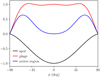 |
Fig. 7 Illustration of the photometric effect of spots, plages, and global effect of an active region accounting for the limb-brightening effect, the limb-darkening effect, and the projection effect. |
5.1.2 Model complexity and computing cost
All the 16 possible models presented above can be implemented as a S+LEAF covariance matrix, The exact rank r of the matrix depends on the model, ranging from r = 15 when using a single mixed population of active regions and Matérn 1/2 decay kernels to r = 90 when using two separated populations for the spots and the faculae and Matérn 3/2 kernels. The cost of the likelihood evaluations of the model scales as O(r2n) (see Foreman-Mackey et al. 2017; Delisle et al. 2022), where n is the total number of measurements (including RV and photometry).
5.2 Statistical Doppler imaging: Proof of concept
In Sect. 5.3.3, we compare the 16 FENRIR physics-based models presented above, together with various data-driven models, in their ability to predict missing data (cross-validation). Here we focus on the two best physics-based models, which both consider spots and faculae as independent populations (sep. model) and use Matérn 1/2 kernels for both the periodic and magnetic cycle components. The best model uses latitude distributions (lat. dist.) of active regions, while the second-best model uses two opposite latitudes (opp. lat.).
We used the samsam MCMC sampler4 (e.g., Delisle et al. 2018) to explore the parameter space. We provide the priors and posteriors of all the parameters explored in Tables 1 and 2. In Figs. 8 and 9, we show a corner plot of the stellar inclination  and the parameters of the distribution of spots and faculae in latitude. We additionally show the full corner plots, as well as convergence diagnostics in Appendix D (see Section 7). Since we observe the Sun from Earth, its inclination is not constant and oscillates through the year
 ![Mathematical equation: $\bar i \in [ - 7,7]$](/articles/aa/full_html/2025/04/aa46391-23/aa46391-23-eq65.png) . The distribution of active regions is typically symmetric with respect to the equator, with µδ ≈ 15° and σδ ≈ 8° (e.g., Mandal et al. 2017). The symmetry with respect to the equator implies that having positive or negative
. The distribution of active regions is typically symmetric with respect to the equator, with µδ ≈ 15° and σδ ≈ 8° (e.g., Mandal et al. 2017). The symmetry with respect to the equator implies that having positive or negative  values yields the same effects. The average absolute inclination through the year is about 4.5°. In both MCMC runs, the inclination is very well constrained to be close to zero, and compatible with the true average value. The average latitude of spots is also restricted to be close to the equator and compatible with the true value. The same is true for the average latitude of faculae. The width of the latitude distribution σδ mostly follows the priors for the spots, which means that it is not constrained by the data. In the case of the faculae, this width seem a bit more constrained towards low values. For both populations, the width is compatible with very small values. It is thus not surprising that the model assuming two opposite latitudes (equivalent to σδ → 0) is performing almost equally well and gives similar results.
In Eq. (18), we express the effect of a spot or faculae on RV as a function of its parameters, in particular the amplitude of their photometric and inhibition of convective blueshift effects. Since here we have a sep. model, we have amplitude terms both for the spots and faculae populations. Since spots are darker regions and faculae are brighter regions, one would expect σspots,phot. < 0, σspots, rv-phot. < 0, σfaculae,phot. > 0,and σfaculae, rv-phot. > 0. Moreover, both kinds of region inhibit the convective blueshift, which would thus result in a net redshift: σspots, rv-cb > 0, σfaculae, rv-cb > 0. Since we consider here a GP approximation of the FENRIR process, the overall sign of the effect is degenerate, but the relative signs of the amplitudes σspots,phot., σspots, rv-phot., and σspots, rv-cb are meaningful. The same is true for the relative signs of the amplitudes for faculae. In Tables 1 and 2, we see that all these signs are correctly recovered, except for σfaculae, rv-phot. which is found to be negative instead of positive. However, this value is constrained to be small compared to the inhibition of the convective blue-shift, and compatible with 0. This is expected since the contrast of faculae is low and their effect in RV is dominated by the inhibition of the convective blueshift.
The decay timescale of faculae (73 ± 8 d) is found to be about twice that of spots (40 ± 3 d). This trend is expected, since during the lifetime of an active region, spots typically disappear after one rotation, while faculae disappear after a few (typically 3-4) rotation periods (e.g., Xu et al. 2017). We note that the model tend to favor having spots appearing at opposite longitudes (αspots, 180 = 0.13 ± 0.05), while this is not true for faculae  . Finally, the magnetic cycle component of the model is dominated by the contribution of faculae (ηspots, mag. ≪ ηfaculae, mag.). As is noted in Appendix C.6, the amplitude of the magnetic cycle term is expected to increase with the typical lifetime of spots/faculae. Since the lifetime of faculae is expected to be longer than the lifetime of spots, we therefore expect their effect to dominate in the magnetic cycle (see e.g., Shapiro et al. 2016).
In Fig. 10, we show the kernel function corresponding to the maximum a posteriori set of parameters for the best physical model. It should be noted that the amplitude and timescale of the magnetic cycle component are degenerated (see the corner plot in Appendix D (see Section 7), which means that the long term component of this kernel (kλ(τ; η) in Eq. (5)) is not well constrained. The short term part (kW(τ; η)kper(τ; η) in Eq. (5)), shown in Fig. 11 is much better constrained. Finally, Figs. 12 and 13 show the GP’s conditional distribution corresponding to the maximum a posteriori set of parameters for the best physical model. The second best model gives very similar results.
This analysis shows that it is possible to perform statistical Doppler imaging, that is, to retrieve the stellar inclination and the average properties of active regions from the statistical distribution of the signal.
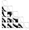 |
Fig. 8 Corner plot of the MCMC samples of the lat. dist. run for the Sun’s inclination and the spots latitude distribution parameters. The dashed lines correspond to the priors. |
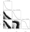 |
Fig. 9 Corner plot of the MCMC samples of the opp. lat. run for the Sun’s inclination and the spots latitude distribution parameters. The dashed lines correspond to the priors. |
Set of parameters explored in the MCMC of the lat. dist. run, with their priors and posteriors (median and 68.27% interval).
5.3 Predictive performance for different kernels
We now turn our attention to the capability of FENRIR kernels to adequately model the data, and whether they perform better than existing models. As a performance metric, we chose the cross-validation score because it is efficient to find a model with a good trade-off between its simplicity and its agreement with the data. Besides the physics-based FENRIR kernels, we also test the following ones.
Set of parameters explored in the MCMC of the opp. lat. run, with their priors and posteriors (median and 68.27% interval).
5.3.1 The FENRIR data-driven model
These kernels are very similar to the physics-based ones, and we still considered a Fourier decomposition up to the third harmonics of the rotation period (Prot./3). However, in the data-driven case, instead of computing this Fourier decomposition from a set of physical parameters, the coefficients of the matrices αk, βk (see Eqs. (33) and (34)) are left free for each harmonic k = 0,…, 3. We performed tests varying the number of modes as defined in Section 4.3. The magnetic cycle is also modeled with free coefficients and always with two modes.
In summary, in this data-driven approach, the two components (active-regions and magnetic cycle) can both be represented as the product of a MultiFourierKernel and a decay kernel. For the magnetic cycle, we only consider the constant part of the Fourier decomposition (up to harmonics zero), while the active-regions part is developed up to the third harmonics. We used two modes for the magnetic cycle and varied the number of modes for the active-regions component.
 |
Fig. 10 Kernel function using the maximum a posteriori parameters from the MCMC of the lat. dist. run. |
5.3.2 Latent GP and derivatives
In order to compare the FENRIR models with more classical approaches, we designed a second set of data-driven models where the active region part is modeled using one or more latent GPs Gk (Aigrain et al. 2012; Rajpaul et al. 2015; Gilbertson et al. 2020; Jones et al. 2022; Tran et al. 2023). The active region component in the channel i (RV or photometry) is modeled as a linear combination of these GPs and their derivatives,
 (39)
(39)
where αi,k, βi,k here are dummy variables, not the same as in Eqs. (33) and (34). We assume an ESP kernel for the GPs Gk. The ESP kernel is an approximation of the widely used squared- exponential periodic (SEP) kernel (e.g., Rajpaul et al. 2015):
 (40)
(40)
This approximation allows for efficient likelihood evaluations (i.e., with a linear scaling with the number of measurements, see Delisle et al. 2022). For the sake of consistency, we develop this approximation up to the third harmonics of the rotation period (Prot./3). We let the hyper-parameters of each latent GP (Pk, ρk, ηk) free and independent of each other. The magnetic-cycle component is modeled as in the FENRIR data-driven case.
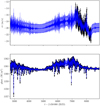 |
Fig. 12 Maximum a posteriori solution of the lat. dist. run superimposed over the RV (top) and photometric (bottom) data. |
5.3.3 Cross-validation tests
In order to compare the ability of different GP kernels to model the Sun’s RV, we designed cross-validation tests. We divide the data into a training set ytrain and a test set ytest. For each kernel, we run an MCMC on the training set and then compute the conditional probability of the test set given the model M:
 (41)
(41)
where η is the set of the model’s hyper-parameters that are explored in the MCMC. The MCMC algorithm allows one to estimate this integral as
 (42)
(42)
that is, the average of the conditional probability computed for each MCMC sample. Finally, the conditional probability for a given sample can easily be computed using its definition:
 (43)
(43)
which is the ratio of the likelihoods of the parameters ηk computed on the full dataset and on the training set.
This conditional probability allows one to compare the different models in their ability to predict the test set from the training set. Here we test our ability to disentangle planetary signatures from stellar activity in the RVs. We thus chose to keep all the photometric data in the training set, and split the RV timeseries between the training and the test sets. Moreover, we are mostly interested in comparing the active-regions component of the models. We thus decided to take eight chunks of 30 d in the RV timeseries for the test set.
We show in Table 3 the results of these cross-validation tests for the three models considered: the physics-based FEN- RIR model (see Sect. 5.1), the data-driven FENRIR model (see Sect. 5.3.1), and the classical case of latent GPs (see Sect. 5.3.2). For the physics-based FENRIR model, we tried the 16 variations of the model described in Sect. 5.1. For the data-driven FENRIR model, we tried to use one or two modes (for all harmonics) and a Matérn 1/2 or Matérn 3/2 kernel (both for the active-regions and for the magnetic cycle). Finally, for the latent GP case, we also tried one or two modes (i.e., one or two independent GPs), and varied the decay kernel for the magnetic cycle component (Matérn 1/2 or 3/2). The kernel of the latent GPs modeling the active regions is always an ESP kernel.
In Table 3, we provide the cross-validation score computed following Eq. (42) in log-scale for each model. This score is thus the log of the average conditional probability over the MCMC samples. Additionally, we provide the median and the 68.27 % interval of the log conditional probability over the MCMC samples. This interval illustrates the dependency of the conditional probability on the hyperparameters. Finally, we provide the RMS of the residuals on the train and test sets.
The best data-driven FENRIR models show slightly better performance than the best physics-based FENRIR. The difference in cross-validation score is of the same order of magnitude as the scatter in score among each model. In contrast, the best latent GP model shows significantly worse performances.
Among, the data-driven FENRIR models, the best performances are obtained when using two modes, which means that there are two independent component in the activity signal.
Among the physical-based FENRIR models, those modeling spots and faculae as two independent populations (sep.) clearly outperform the mixed populations models (mix.). The reality is in between those two extreme cases; that is, there is some correlation in the appearance of spots and faculae, and in particular some active regions consist of a spot surrounded by faculae, but this is not always the case. Our result suggest that considering spots and faculae as two independent populations is a better approximation. As discussed in Sect. 5.2, in the sep. case, while the latitude distributions of both types of active regions are similar, the decay timescale of spots is about half the decay timescale of faculae. This might explain why the sep. model is preferred over the mix. model, which inherently assumes that spots and faculae in the same active region appear and disappear at the same time. Regarding the latitude distribution (lat. dist. or opp. lat.), the two alternative models show very similar performances. As shown in Sect. 5.2, while the average latitude of active regions can be constrained, the width of of the distribution is not well constrained, which might explain the similar performances of both models.
The Matérn 1/2 kernel seems to be slightly preferred over the Matérn 3/2 kernel, both for the active regions component and for the magnetic cycle component, and both in the physics-based model and in the data-driven model.
5.3.4 Cross-validation tests using additional activity indicators
While in this article we derived the physics-based FENRIR model for RV and photometry only, the approach is more general and could be extended to additional activity indicators. Such an extension of our physics-based model is beyond the scope of this article. However, the data-driven FENRIR model, as well as the classical latent GPs approach, can readily be extended to any additional channels. We thus ran a larger series of crossvalidation tests, using the activity indicators extracted from the HARPS-N solar spectra at the same time as the RVs as provided by Dumusque et al. (2021).
We use the exact same splitting of the HARPS-N RVs between the training and test sets, and use different combinations of photometry and activity indicators as additional training data. Because we compute the conditional probability on the same RV test set, we can directly compare the cross-validation scores for any model and any set of activity indicators.
We tested all the possible combinations of photometry, full width half maximum (FWHM), bissector span (BIS),  , both with the data-driven FENRIR model and the classical latent GPs model, with one or two modes in both cases and with Matérn 1/2 or 3/2 decays for the active regions and magnetic cycle parts.
The 30 best models, in terms of cross-validation scores, are shown in Table 4, while the full list is shown in Appendix E (see Section 7). We also show in Fig. 14 the GP’s conditional distribution corresponding to the maximum a posteriori set of parameters for the best model (data-driven FENRIR GP with a single mode and trained on the FWHM and BIS indicators).
Here are a few comments inspired by these results:
The best cross-validation scores (Table 4) are significantly higher than the scores obtained using only the photometry as activity indicator (difference of about 16 in log, i.e., a factor of about 7 × 10⁶);
The bissector span is used in the 29 best models, which indicates that this activity indicator is particularly helpful in predicting RVs;
The FENRIR data-driven model seems to better predict RVs than the latent GPs model. However, it should be noted that the FENRIR data-driven model has a larger number of hyperparameters, since the amplitudes of all the harmonics of the rotation period are left free. While solar data allows one to constrain well these parameters, and to prevent overfitting (which would result in decreasing the cross-validation score), it might be more challenging to constrain them on smaller datasets.
The models with a single mode (as defined in Section 4.3) perform well, even when multiple activity indicators (except for the photometry) are included in the models: it is sufficient to model the data as if there were only one type of “average active region”, which appears at random times.
The Matérn 1/2 and 3/2 kernels seem to give similar predicting performances, while the computational cost of the Matérn 3/2 kernel is typically nine times larger.
Cross-validation tests for the active-regions component of the model trained on Sun RV + photometry.
6 Discussion
Our statistical model of stellar activity was built in three steps. First, we defined the FENRIR model in Section 2.3. Second, in Section 3, we made further assumptions on the impulse response, distribution of feature parameters, and rate of apparition of magnetic regions (Poisson rate). The validity of the assumptions in these two first steps is the object of Section 6.1. Third, we approximated FENRIR processes by a Gaussian distribution. This approximation is discussed in Section 6.2. In Appendix F, we present three additional discussions: the construction of relevant activity indicators, the potential relationship between phase shifts in RV and photometry with the faculae-to-spot ratio, and the application of our work to classical Doppler imaging.
6.1 Model assumptions: Limitations and novelty
In the FENRIR model, detailed in Section 2.3, the emergence times of magnetic regions follow a Poisson process (Eq. (6)). This means that the probability of a magnetic region appearing is independent of the presence of other active regions. However, this assumption does not fully hold, at least for the Sun, where active regions tend to emerge near existing ones and on active longitudes (e.g., Berdyugina & Usoskin 2003; Borgniet et al. 2015). Despite this, as discussed in Section 3.1, the issue is partially mitigated by considering impulse responses as groups of magnetic regions rather than individual ones. In our implementation, we account for spots shifted by 180°, which helps address this limitation.
We further specified the assumptions on the impulse response, distribution of feature parameters and Poisson rate in Section 3. Assumptions 1–6, outlined in Section 3.4, are common to the physics-based and data-driven models.
We assumed that the star has a solid body rotation (Eq. (23)). However, the angular velocity of the solar surface depends on the latitude, a phenomenon known as differential rotation (Gray 2005). With a preliminary analysis, we found that the firstorder effect of differential rotation is to reduce the time scale of the window kernel: the signal loses coherence more quickly.
Although the assumption that spot properties are independent of their position seems reasonable (Eq. (22)), it is known that their lifetime, size, and position depend on when they appear in the magnetic cycle (e.g., Song et al. 2024). First, at minimum solar activity, sunspots appear on average at a latitude 30-45° away from the equator. As the activity level rises, the average latitude of sunspots moves towards the equator. Second, the ratio of spots to faculae coverage varies with stellar activity (Nèmec et al. 2022), so that the parameters governing their effects should depend on time in a non-stationary way. This is further supported by the observation that if GP models are fitted to the solar HARPS-N RVs, the hyperparameters change significantly over time (Klein et al. 2024). While the general model can account for it (Eq. (7)), assumption 4 in Section 3.4 contradicts it. A possible workaround is to divide the data in shorter time intervals, such as months or years, and fit the model independently on each part.
In addition, we made several assumptions specific to the physics-based model (Sections 3.1–3.3). We computed the total RV as the sum of local stellar RVs weighted by their relative flux, which is simplistic. In Appendix B.3, we derived the expressions of RV, as well as ancillary indicators considering that the measured cross-correlation function (CCF) is a weighted sum of the local stellar CCFs, as is done in SOAP 2.0 (Dumusque et al. 2014). This formalism takes into account in particular the interdependence of velocity, contrast, and CCF width. Our model is also too simplistic for large spots, which cannot be assumed to be point-wise.
The lifetime of magnetic structures is correlated with their size, as documented by Meyer et al. (1974); Martinez Pillet et al. (1993). While our mathematical framework can accommodate this relationship, it is not currently incorporated into our physicsbased model implementation. Additionally, the influence of the magnetic network is not considered in our model (see Borgniet et al. 2015, for a discussion of its effect).
Our framework, despite its limitations, introduces several innovations. Traditionally, the representation of stellar activity in photometry and spectroscopy as a joint Gaussian Process (GP) relies on qualitative arguments (Aigrain et al. 2012; Gilbertson et al. 2020; Jones et al. 2022; Tran et al. 2023), resulting in the latent GP model in Eq. (39), possibly with higher order derivatives. In contrast, our approach offers a quantitative, physics-based model for understanding stellar activity in both photometry and spectra.
GP frameworks based on a quantitative physical models have been proposed. In Luger et al. (2021b,a) the goal is to retrieve an intensity map of the surface from photometric and spectroscopic measurements, respectively. In both cases, the GP represents the intensity pattern on the stellar surface and its uncertainties. The star rotates, but this pattern is considered fixed during the time span of the observations. Our framework focuses on modeling the evolution of stellar surfaces over time, and is more akin to Luger et al. (2021a). They start from a GP model of the stellar surface, and through a linear mapping, they derive a GP representation of photometric time series. Our framework has a different starting point, summarized by Eqs. (6)–(8). A comprehensive comparison of the two methods is beyond our current scope. We simply note that our framework extends to spectroscopy, accounts for the inhibition of the convective blueshift, incorporates variations due to the magnetic cycle, and enables likelihood evaluations scaling as O(N). Additionally, our approach features representations of non-Gaussianity, which we now explore.
Cross-validation tests for the active-regions component of the model trained on Sun RV and various activity indicators.
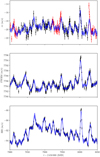 |
Fig. 14 Maximum a posteriori solution of the best (in terms of crossvalidation score) data-driven FENRIR model superimposed over the RV (top), FWHM (middle), and BIS (bottom) data, zoomed on a few rotation period. The train set is highlighted with black points, while the test set is highlighted with red points. |
6.2 Are stellar activity signals Gaussian?
A stochastic process X(t) is said to be a GP if for every finite collection of times t1,…, tn, then X(t1),…, X(tn) has a Gaussian multivariate distribution (Rasmussen & Williams 2005). The FENRIR GPs used in Section 5 satisfy this definition, but as mentioned in Section 2.4 they are only an approximation of the FENRIR models. We now discuss whether this is a good approximation.
There is a simple argument against stellar activity signals being strictly Gaussian. Indeed, if X(t) is a GP of vanishing mean, X(t) and –X(t) have exactly the same covariance, and thus the same probability. However, the signature of the inhibition of the convective blueshift on RV is not symmetrical, it always manifests as a net redshift (see Fig. 3 (b2)). Furthermore, as soon as there is an excess of the effect of regions brighter or darker than the quiet surface, the flux effect does not have a symmetric distribution. This type of non-Gaussianity could be called “spatial” and would manifest as a non-Gaussian histogram of RV and photometric observations.
Non-Gaussianity can also manifest in the temporal structure of the signal. If we were to generate several realizations of a GP, and compute the Fourier transform, it would appear that the phases are uniformly distributed on [0,2π]. In particular, phases at two different frequencies are statistically independent. In the case of stellar activity, we expect phases to be tied to each other. Suppose that only spots appear at a given latitude, and very rarely. This means that each time a spot appears, the difference between the phases of the process at the stellar rotation period and its harmonics is not only not uniform, but deterministic.
To study both spatial and temporal non-Gaussianity of stellar activity signals, we briefly introduce the notion of cumulant (for more details see Mendel 1991). Considering a stochastic process X(t), given n time stamps (ti)i=1,…,n the cumulant generating function of X(t1),…, X(tn) is
 (44)
(44)
In the Taylor expansion of  as a function of xis, the cumu- lant of order n, κn, is the coefficient of their products, x1 x2…xn. The cumulant κn is thus a function of (ti)i=1,…,n and is often referred to as the n-point correlation function. One of the properties of stationary GPs is that their cumulants of order three or greater are equal to zero.
A stationary process is such that the distribution of X(t + τ1),…,X(t + τn) does not depend on t. When the FENRIR process is stationary, its n-point correlation function, or cumulant of order n is expressed as a function of time lags between n – 1 points and a reference one. In Appendix A.2, we show that the cumulant of order n can be analytically derived from the FENRIR model (Eqs. (6)–(8)),
 (45)
(45)
Applying the Fourier transform to Eq. (45), we obtain the polyspectrum of our FENRIR process,
 (46)
(46)
where  is the Fourier transform of g(t, γ) considered as a function of time t. Like cumulants, polyspectra of GPs vanish at order three and beyond. We now discuss “spatial” and “temporal” non-Gaussianity in Sections 6.2.1 and Sections 6.2.2.
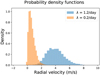 |
Fig. 15 Histogram of RVs simulated with a FENRIR process, with a rate of λ = 1.2 and λ = 0.2 magnetic region appearing per day (respectively the blue and orange histograms). |
6.2.1 Poisson rate and asymmetry
We might anticipate that increasing the rate of feature appearance enhances Gaussianity. At low Poisson rates, only one feature is present at a time. However, as the rate increases, multiple features begin to overlap, blurring phase information, and bringing the system closer to the conditions described by the central limit theorem.
As an illustration, we generated FENRIR processes using the same properties as in Section 3.3, with a sampling of one point per day over 20 years. We used two Poisson rates, λ: 1.2 and 0.2 magnetic regions appearing per day. The histograms of the simulated RVs are shown in Fig. 15. The RVs simulated with λ = 1.2 d–1 appear closer to a Gaussian distribution than those with λ = 0.2 d–1. To highlight this more clearly, we subtracted the mean from each simulated RV time series and normalized them by their standard deviations. Figure 16 displays the histogram of these normalized RVs. As anticipated, the distribution of RVs with λ = 1.2 d–1 is closer to a normal distribution. As a remark, Fig. 15 shows that the variance of the simulated RVs increases with λ, which is expected from Eq. (11).
The FENRIR simulations, based on Section 3, are designed to approximate the characteristics of the Sun’s magnetic regions. These simulations can be compared with a three-year time series of RVs measured by HARPS-N (Dumusque et al. 2021). We binned these measurements every 15 hours and subtracted a 9th-order polynomial, thus removing frequencies lower than approximately 1 year, to avoid masking the contribution of stellar rotation. Fig. 17 displays the histogram of the residual RVs, which exhibits a similar behavior to the FENRIR processes: a sharp cut-off at negative RVs, heavier tails at positive RVs, and a maximum slightly shifted towards negative RVs. This behavior is independent of the degree of the fitted polynomial. However, as expected, when binning is done over shorter intervals, high- frequency noise tends to make the RV histogram slightly more Gaussian.
The λ = 1.2 d–1 value is chosen to reproduce a Wolf number of ~50, and was calibrated to have the same standard deviation as the measured solar RVs, 1.23 m/s. Interestingly, while nothing was fine-tuned in the model to achieve this, the simulated and measured RVs have very similar empirical third-order moments: 1.02 m3/s3 and 0.91 m3/s3, respectively. Generating Gaussian noise with the same sampling as the solar 15-hour binned RVs, and using the same covariance (estimated via Fast Fourier Transform of solar RVs), yields a standard deviation of the third-order moment of 0.18 m3/s3. This indicates that the third-order moment of the measured RVs is non-zero with a 5σ significance and is accurately reproduced by the FENRIR model.
The fact that Gaussianity increases with λ can be qualitatively understood based on Eqs. (45) and (46). We consider a stationary FENRIR process, and its GP approximation. The two processes have identical first and second-order cumulants. Since the GP is stationary, from Eq. (45), its variance at each time σ2 would be constant, proportional to λ. If we were to estimate empirically the cumulants of this GP, they would zero because of statistical fluctuation. The standar the cumulant of order n of a GP is proportional turn to λn/2, while all cumulants of order n are proportional to λ. Consequently, the ratio of the cumulants of order n ⩾ 2 of the FENRIR process and its GP approximation is proportional to λ/λn/2. This tends to zero when λ increases for all n ⩾ 3: the FENRIR process becomes more and more indistinguishable from its GP approximation.
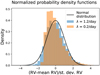 |
Fig. 16 Histogram of normalized RVs simulated with a FENRIR process, with a rate of λ = 1.2 and λ = 0.2 magnetic region appearing per day (respectively the blue and orange histograms). RVs are normalized by subtracting the mean of the time-series and dividing by its empirical standard deviation. The black line represents a Gaussian distribution with vanishing mean and variance 1. |
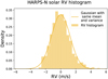 |
Fig. 17 Yellow histogram: Histogram of RVs measured on the Sun (public data Dumusque et al. 2021) by HARPS-N after binning by 15 hours, and fitting and subtracting a 9-th order polynomial. The solid yellow curve is a Gaussian ditribution with the same mean and variance as the data. |
6.2.2 Bispectrum
We now turn to “temporal” non-Gaussianity. Here, we do not study measured RVs, but only quantify the non-Gaussianity of FENRIR models. We use the polyspectrum of order 2, called the bispectrum. From Eq. (46), we obtain its expression for a FENRIR process,
 (47)
(47)
 (48)
(48)
The bispectrum is a function of the Fourier transform of the impulse response g, which can be expressed as a product of what we called a window function, modulating the amplitude of the signal as the region grows and decays in size, and a periodic term (see Eq. (23)). We first assume that the window term is constant (the size and brightness of the magnetic region are constant). The periodic part can be expressed as a truncated Fourier series
 (49)
(49)
This means that the Fourier transform of g is only non-zero at frequencies kω, k = –d, …, d, and the only non-zero products in the integrand of Eq. (47) are such that ω1 = k1ω and ω2 = k2ω2 such that k1, k2, and –(k1 + k2) are all integers between –d and d.
Even if a cumulant is non-zero, its value estimated from noisy data could be compatible with zero. To evaluate this, we consider that the amplitudes of  are estimated with an uncertainty. From there, we compute the mean squared error on s(ω1, ω2, γ) defined in Eq. (48).
In Fig. 18, we show the ratio of s and an upper bound on its mean squared error with the model of Section 3, assuming an inclination  , a latitude δ = 0, and a ratio between the photometric RV and convective blueshift inhibition effects B = 1. We assume that
  is known with a 15% accuracy for all ω, and the uncertainties on
  , are independent. It appears that several bispectrum coefficients are more than three times greater than their mean squared error.
The bispectrum shown in Fig. 19 concerns a single magnetic region with a fixed latitude and a given stellar inclination. In Fig. 19, we show the real part of Eq. (48) for ω1 = ω2 = ω as a function of inclination  and latitude
  means that the one pole of the star is pointing to the observer, and
  , the other pole,
  means the stellar rotation axis is perpendicular to the line of sight. For each inclination, only regions satisfying
  are visible (see Appendix B). The bispectrum (Eq. (47)) requires to perform an integration. In the bottom of Fig. 19 we show the value of the integrand Eq. (48) averaged over latitude, assuming that all latitudes are equally probable. It appears that the real part of the bispectrum does not average out for most inclinations.
In the case where the window function (growth and decay of the spot area) is taken as non constant, thanks to the convolution theorem, the Fourier transform of g is
 (50)
(50)
Taking into account the window function would give a smoothed version of Fig. 18, but would not necessarily mask non- Gaussianity.
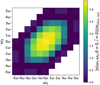 |
Fig. 18 Absolute value of the bispectrum divided by an upper bound on its mean squared error, for a purely periodic, equatorial spot signal with a contribution of the convective blueshift inhibition twice that of the RV photometric effect, and |

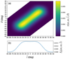 |
Fig. 19 (a): Real part of Eq. (48), ω, ω coefficient as a function of stellar inclination |

7 Conclusion
Our primary goal was to represent the signal induced by stellar activity as a stochastic process, derived from a quantitative physical model. We consider a general case where the data consist of observations of a given star in the form of one or several time series, which may vary in nature and are not necessarily sampled at the same epochs. These include radial velocities (RVs), photometry, activity indicators, or even timeseries of spectra used in transit spectroscopy or Doppler imaging. The FENRIR model, developed in this article, provides a joint likelihood representation of these observables: their probability distribution given the model parameters η, which include the sky-projected obliquity, average latitude of the spots, and rotation period.
The FENRIR model is built upon three key ingredients. (1) the impulse response: the effect of a given stellar feature (such as a spot or plage, or groups of them) as a function of its parameters (e.g., size, latitude). (2) The statistical distribution of feature parameters, given the average properties of the star, the parameters of the likelihood η. (3) The rate at which features appear, which may vary over the magnetic cycle.
The FENRIR model is generally not Gaussian, but it can be approximated by a Gaussian distribution. The resulting FENRIR GPs can be used like other GPs, here with hyperparameters η. We provide a public implementation in two flavors5, physicsbased and data-driven (see Section 3). In the first case, starting from a physical model, we specify the three ingredients of the model for the joint analysis of RV and photometry. The data- driven version considers the impulse response as a vector of free parameters, and can be used on any combination of observables.
FENRIR GPs are computed in the S+LEAF framework (Delisle et al. 2020, 2022). This enables fast likelihood evaluations, with a cost proportional to the number of observations.
Our goal is twofold: first, to improve the accuracy of stellar activity models, in order to improve exoplanet detection capabilities; and second, to constrain the statistical distribution of spots and faculae on slow rotating stars. To test the performance of FENRIR GPs, we analyzed data acquired on the Sun, SORCE photometry, and the first three years of HARPS-N spectroscopic observations (Dumusque et al. 2021). We tested the predictive accuracy of FENRIR models with cross-validation, on RV and photometry only, and on RV, FWHM, BIS, and photometry time series. In both cases, FENRIR models performed better than latent models with a GP and its derivatives. Second, using a separate process for spots and faculae, based solely on photometry and RVs, we retrieved the solar inclination with a precision of ~5°, as well as realistic spot and faculae distributions, close to the equator. This serves as a proof of concept, but further testing should be performed to ensure that our method gives reliable results on other stars.
The FENRIR framework is versatile. Here, we considered 16 variants of the physics-based model, but many more options are possible. It could be adapted to include differential rotation, and more subtle effects of spots and plages (see e.g., Dumusque et al. 2014). The FENRIR framework allows one to interpret the non-Gaussianity present in the solar data (see Section 6.2), and should, in the long run, allow one to go beyond the GP framework. In Appendix F, we also discussed several aspects: building relevant activity indicators, interpreting phase shifts between RV and photometry or log  as a signature of the ratio of spots and plages filling factors, using FENRIR in classical Doppler imaging. These avenues will be explored in future works.
Data availability
Appendices D (MCMC convergence tests and corner plots) and E (full table of cross-validation results) are available on Zenodo at https://doi.org/10.5281/zenodo.14919319.
Acknowledgements
This work has been carried out within the framework of the NCCR PlanetS supported by the Swiss National Science Foundation. We acknowledge financial support from the Swiss National Science Foundation (SNSF), grant number: 205010. The authors warmly thank Xavier Dumusque, Vincent Bourrier, Christophe Lovis, Nadège Meunier, Lionel Garcia, Sophia Sulis and Olivier Flasseur for their helpful suggestions. We thank Suzanne Aigrain for her careful review of our article and her insightful comments.
Appendix A Covariance and cumulants
A.1 Covariance in the general nonstationary case
In this appendix, we compute the mean and autocovariance of FENRIR processes. These expressions are particular case of the general formula for cumulants, derived in Section A.2. Since the manipulation of cumulants might be unfamiliar to our readers, here we give an alternate calculation. For simplicity, we refer to the magnetic regions appearing on the star (spots and faculae, or groups of them) as features.
We consider that the features appear independently on a time interval [–L/2, L/2] with rate λ(t). Then the times of feature appearance follow the distribution  . The signal in a given observational channel is modeled as
 (A.1)
(A.1)
and we denote by y(t) the limit in probability of yL(t) as L tends to infinity (yL(t) is a random variable). Here n is the number of features such that tk ∈ [–L/2, L/2], and follows a Poisson distribution of parameter  . To compute the covariance of y, which by definition is
 (A.2)
(A.2)
We first compute the expectancy of the value of y at a time t,  , then
  . In both cases, we do the calculation for yL and let L tend to infinity.
We first note that with our hypotheses, the probability of parameters {γ}n = γ1,…,γn knowing the times of arrival of features {t}n = t1,…, tn can be written

As a consequence, from the law of total probability,
 (A.3)
(A.3)
And we have
 (A.4)
(A.4)
So
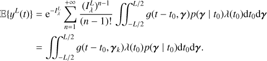 (A.5)
(A.5)
Provided this integral converges when L tends to infinity,
 (A.6)
(A.6)
We now compute the expectancy of the product yL(ta)yL(tb). Here also, provided the infinite sum and integral can be inverted, since for k ≠ j, tk and tj are statistically independent,
 (A.7)
(A.7)
 (A.8)
(A.8)
 (A.9)
(A.9)
Since there are n(n – 1) pairs of k, j where k ≠ j,  can be written as the sum of two terms CL and DL,
 (A.10)
and
 (A.11)
We note that as L tends to infinity, provided the integral over tk converges, CL(ta, tb) is the product of  and
and  . If DL(ta, tb) admits a limit as L tends to infinity, the covariance of y is
 (A.12)
In this formula, the distribution of γ can depend on to.
We note that if we replace y(tb) with z(tb) where z models the effect of stellar activity on another ancillary indicator,
 (A.13)
the reasoning is unchanged, and provided all the limits when L tends to infinity converge,
 (A.14)
A.2 Cumulants and polyspectra
A.2.1 Purpose
In this Section, we compute the analytical formula of the cumulants and polyspectra of the FENRIR process y(t), defined as
 (A.15)
For a stationary FENRIR process, the autocovariance is of the form  . Even if the γ can take only one value, the knowledge of k(τ) does not give unequivocally g: several functions can have the same autocorrelation. If y(t) is Gaussian, based on it the best we can do is to estimate k(τ). If y(t) is non-Gaussian we can characterize g more precisely, thus have not only less biases but also leverage more information. The purpose of cumulants is to reveal non-Gaussian behaviors.
The cumulant generating function of y(t1), y(t1)…, y(tn) is
 (A.16)
In the Taylor expansion of K as a function of αis, the cumulant of order n, κn, is the coefficient of their products, α1α2…αn. Considered as a function of t1,t2,…, tn it is sometimes called the n point correlation function. For a GP, cumulants of order three and four are zero. Our main result is that
Theorem 1. For a FENRIR process y(t) defined as in Eqs. (6)- Eqs. (8), the cumulant of order n is
 (A.17)
The covariance is the 2-point correlation function. When GPs are stationary, we have κn(t1, t2) = κn(|t1 – t2|) they are equivalently represented by the Fourier transform of the kernel κ(τ): their power spectrum density (PSD). Similarly, under the hypothesis of stationarity of the process, the quantity κn(t, t + τ1,…, t + τn–1) does not depend on t. Considering the n point correlation function as a function of the n – 1 variables τ1, …,τn–1, we can define the polyspectra as the n – 1 dimensional Fourier transform of κn(t, t + τ1,…, t + τn–1).
The proof of Eq. (A.17) can be modified straightforwardly to prove a more general result,
 (A.18)
where gi(t) are impulse responses associated with channel i. This expression generalizes Eq. (A.14). This expression has the advantage to be valid if the process is non stationary, and can explore non-Gaussian dependencies across channel. However, it is unlikely that all these aspects could be explored simultaneously in a practical way.
In the case where patterns appear with a constant Poisson rate, and the distribution followed by γ(tk) does not depend on time, γ(tk) ~ p(γ), the stochastic process y(t) is stationary. We can write Eq. (A.17) as a function of time differences τi = ti – t1. With the change of variable t ← t – t1,
 (A.19)
In that case, the Fourier transform of κn as a function of τ1, …,τn–1 is called the polyspectrum of order n. Here, provided the integrals on γ and τ1,…, τn–1 can be inverted, it is equal to
 (A.20)
The purpose of polyspectra can be understood by recalling that stationary GPs are completely characterized by their power spectral density, which is the Fourier transform of the kernel. Under mild conditions (Bloomfield 2004), the power spectral density has another interpretation: It is the mathematical expectancy of the squared modulus of the Fourier transform of the process. Stationary GPs thus have completely random phases. Suppose we compute the phase of a stationary GP between times t1 and t2 on the one hand and between times t3 and t4 on the other hand, such that t3 – t2 is much greater than the process correlation, the phase obtained on the first and second time intervals are statistically independent. For stationary GPs, for all n ⩾ 3, Eq. (A.20) should be equal to zero for all choice of frequencies ω1,…, ωn–1. As a consequence, significantly non-zero polyspectra indicate non-Gaussianity. We consider a quantity ν and all combinations of n – 1 frequencies such that 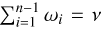 . In Eq. (A.20), the phase of the Fourier transform evaluated at ν can be seen as a point of reference. If the frequencies ω1, …,ωn–1 and v are not independent, the poly spectrum is non-zero.
A.2.2 Proof
To establish Eq. (A.17), we use several properties of cumulants, outlined below.
Theorem 2. We consider n random variables Y1, Y2,…, Yn (defined on the same σ algebra). (i) Cumulants are multilinear, for all i, for two real numbers a and b,  .
.
(ii) If there are at least two indices i , j such that Yi and Yj are independent, κ(Y1,…, Yi,…, Yj,…, Yn) = 0.
(iii) If N is a random variable following a Poisson distribution of parameter Λ, κ(N, N…, N) = Λ regardless of the number of times N is repeated.
(iv) Law of total cumulance. Suppose that we have a random variable Y and we can define the conditional distribution of Yis knowing X. Then
 (A.21)
where  means that π runs through all the possible partitions of indices of indices {1,…, n}. B ∈ π means that B runs through the blocks of permutation π and κ(Yi : i ∈ B | X) is the cumulant of Yi : i ∈ B knowing X . To understand (iv), suppose we want to compute κ(Y1, Y2, Y3). The partitions of our indices {1, 2, 3} are {{1}, {2}, {3}}, {{1}, {2, 3}}, {{2}, {1, 3}}, {{3}, {1, 2}}, {{1, 2, 3}}.
In the partition {{1}, {2}, {3}} we have three blocks, {1}, {2} and {3}. In the partition {{1}, {2, 3}} we have two blocks, {1} and {2, 3}. For n = 3, the law of total cumulance then writes

where the quantities κ(Yi : i ∈ B | X) are random variables because they are functions of the random variable X .
(v) With the same notations, the link between cumulants and non centred moments is the following
 (A.22)
For instance

Formulae (A.21) and (A.22) are similar. In the first case one takes the cumulants over the different blocks of the distribution, in the second one simply takes the product. This will be useful in the proof of Eq. (A.17).
Proof of Eq. (A.17): We consider n times ordered increasingly T1,…, Tn. We suppose that g has a finite support, meaning that for some T, for t outside [–T/2, T/2], g(t, γ) = 0. Because g has a finite support, computing the n-th order cumulant of y(T1), …,y(Tn) for y as defined in Eq. (A.15) is equivalent to compute the cumulant of the variables Yi
 (A.23)
where features appear at tk, following a Poisson process between t1 – T/2 and tn + T/2 with a variable rate λ(t), and we define the random variables G(Ti – tk) = g(Ti – tk, γ(tk)) to simplify notations. N is the number of features in this interval and follows a Poisson distribution with parameter  . A feature appearing at time tk has parameters drawn from the distribution p(γ, t).
In this expression, k(Gi : i ∈ B) are not random variables, but constants. Thanks to the multilinearity of cumulants (property (i) in Theorem (2)), we have
 (A.24)
Measurable functions of independent variables are independent. Since ti and tj are independent for i ≠, j, G(T1 – ti) and G(T1 – tj) are not independent if and only if i = j. Now, because cumulants are zero if two or more variables are independent (property (ii) in Theorem (2)),
 (A.25)
if and only if i1 = i2 = … in, and
 (A.26)
The ti, i = 1..Ns are drawn independently from the same distribution, so for a given k, all the G(Tk – ti), i = 1..N are drawn from the same distribution: κ(G(T1 – ti),…, G(Tn - ti) | N) = κ(G(T1 – tj),…, G(Tn – tj) | N) for all i, j = 1..N and
 (A.27)
Thanks to the law of total cumulance (property (iv) in Theorem 2),
 (A.28)
Injecting Eq. (A.27), denoting by Gk = G(Tk – t), we have
 (A.29)
Here κ(Gi : i ∈ B) is a constant, not a random variable. Thanks to the multilinearity of cumulants (i), we have
 (A.30)
where  where N is repeated |Bπ| times, the number of blocks in partition π. For a Poisson distribution of parameter Λ, κ(N,…, N) = Λ (property (iii) in Theorem (2)). We now have
 (A.31)
and thanks to the link between moments and cumulants (property (v) in Theorem (2)) we can write
 (A.32)
Finally, by definition of  ,
,
 (A.33)
canceling Λ in Eq. (A.32), and recognizing that because of the finite support of g, the integral (A.33) is unchanged if we take as lower and upper bounds –∞ and +∞, and is true for any T, we can thus extend our results to functions with infinite support and we have the desired result,
 (A.34)
Appendix B Analytical approximation of the spot/facula RV effect
B.1 Weighted radial velocity (RV)
In this appendix we approximate the RV and photometric effect as follows. We assume that the RV effect on the data of the quiet stellar surface is
 (B.1)
(B.1)
where x is the position on the visible disk, V(x) is the local velocity, F(x) the local flux, F0 the flux integrated on all the stellar surface and eobs the unit vector pointing from the observer to the star. Where
 (B.2)
(B.2)
where Vcb is the velocity modulus of the convective blueshift effect, er is pointing radially outwards, ω is the rotation axis times the rotational velocity and r is the vector joining the stellar center and the point at position x on the stellar surface.
Denoting by RVmag(t) the RV when a magnetic region is present, and by V′(x) and F′ (x) the velocity and flux fields ,
 (B.3)
(B.3)
where
 (B.4)
(B.4)
 (B.5)
(B.5)
We are interested in the difference between RVmag(t) and RVquiet(t). Developing  at first order in ΔF, we have
 (B.6)
(B.6)
 (B.7)
(B.7)
 (B.8)
(B.8)
The term ycb and yph are respectively called the inhibition of convective blueshift term RV photometric terms.
Assuming that the magnetic region is small, the flux can be written as product of the flux per surface unit f (x) times the projected area of the magnetic region, W(x)P(x) where W(x) is the intrinsic area and P(x) the projection effect, times the limbdarkening effect l(x). We write
 (B.9)
(B.9)
 (B.10)
In the following, we establish the expression of the flux and RV as a function of the position of the magnetic region (longitude ϕ and latitude δ) on an inclined star. For small spots, we can neglect the ΔF/F0 term in Eq. (B.7) (it is second order).
We model the surface of the star by a sphere and consider that a spot or facula is point-like. For the sake of simplicity, in the following we simply refer to a spot, but the reasoning for a facula is identical. We consider a direct frame x, y, ɀ such that x points in the direction of the observer and y, ɀ defines the sky plane.
We first assume that the rotation axis of the star is aligned with ɀ denote by ϕ, δ the spherical coordinate of the center of a spot, such that its position in the Cartesian frame is
 (B.11)
 (B.12)
 (B.13)
The local frame (u, υ, w) at (x, y, ɀ) is such that
 (B.14)
 (B.15)
 (B.16)
The effect of a spot on the RV depends on the inclination of the star with respect to the plane of the sky  . To compute the position of the spot and the projection of the local frame centered at the spot in the reference frame, we apply a rotation of axis y and angle
 ![Mathematical equation: $\bar i \in [0,\pi /2]$](/articles/aa/full_html/2025/04/aa46391-23/aa46391-23-eq329.png) . We now have
. We now have
 (B.17)
 (B.18)
 (B.19)
and
 (B.20)
 (B.21)
 (B.22)
We assume that the effect of the spot is proportional to its projected area onto the sky plane times a velocity projected onto the x axis (more precisely -x axis, since the velocity is assumed to be positive in the direction observer - star) multiplied by a limb-darkening effect. In the case of the photometric effect, the velocity in question is the velocity of the stellar surface due to the stellar rotation in the rest frame, it is therefore the υ component of the velocity. The convective blueshift inhibition effect is due to the motion of the gas from the center of the star to the stellar surface. We are therefore interested in the u component of the velocity projected onto x. The spot position on the stellar surface changes its projected surface onto the sky plane. The correction factor is equal to the Jacobian of the projection from the (υ, w) onto the (y, ɀ) plane, from Eq. (B.21) and Eq. (B.22), the projected area of the spot is proportional to
 (B.23)
The factor J actually coincides with the distance to the center of the star normalized by the stellar radius, µ. In the following we keep the notation µ, which is widely used for limb-darkening laws. The spot is visible if its position is such that x ⩾ 0. From Eq. (B.17), this translates to the condition
 (B.24)
Overall, the velocity contribution of the photometric and inhibition of convective blueshift effects on RV (yph and ycb , and its effect on photometry ɀph is 0 when (B.24) is not satisfied, and when it is:
 (B.25)
 (B.26)
 (B.27)
We can parametrize the intrinsic area of the feature with a timescale ρ. For instance, if we choose a one-sided exponential, W(t) = 1t⩾0e−t/ρ where 1t⩾0 equals 0 for negative t, and one for positive t. In the remainder of this appendix, we ignore the W(t) term.
ΔF is the flux difference between the stellar surface and the spot and f★ is the mean stellar flux, ω is the local rotational velocity of the star and R★ is the stellar radius, Δ VCB is the difference between the velocity of the plasma in the u direction with and without convective blueshift inhibition. The + sign comes from the fact that we are projecting u and v onto −x, and the inhibition of convective blueshift has a positive velocity in the −u direction. The photometric effect can be positive or negative depending on whether the area under consideration is brighter of darker than the quiet surface of the star. The symbol l represents the limb-darkening, which is typically a function of µ. For an equatorial spot,  , and without limb-darkening, we simply have
 (B.28)
 (B.29)
In the case of a non constant limb-darkening law l(µ), the expressions (B.25) and (B.26) are particularly simple if l is of the form
 (B.30)
In the general case the photometric and convective blueshift inhibition effect are summed. For the sake of simplicity we write their contribution up to a multiplicative factor and denote the relative contribution of the photometric effect compared to the convective blueshift inhibition as B. The combined effect on the RV is then
 (B.31)
for ϕ satisfying (B.24) and 0 otherwise.
When the limb darkening law is taken as a constant, the general formula for the RV effect of a spot is
 (B.32)
For a constant rotation rate, constant δ, we have ϕ = ωt. We can rewrite g as
 (B.33)
where c0 , c1 , c2 , s1 , s2 are coefficients that depend on  , δ and B. As a concluding remark, we note that because the limbdarkening is in power of µ, itself an affine function of cos ωt. Regardless of the order of the limb-darkening law chosen, we can always write g in the form
 (B.34)
The next section provides a formal justification of this claim.
B.2 Fourier decomposition of the periodic part
We denote by I and J the impulse responses in channels i and j. For simplicity, we write them I(t, γ) = W(t, γ)i(t, γ) and J(t, γ) = W(t, γ) j(t, γ) where i(ϕ, γ) and j(ϕ, γ) are the periodic parts, which can be written in the form
 (B.35)
where 1vis. is the indicator function of the spots visibility (equals to one when the spot is on the observer’s side of the star, 0 otherwise), and i0, j0 describe the effect of the feature without visibility considerations. The Fourier expansions of the effect of the feature, including the limb-darkening effect, are provided in Appendix B. Overall, this can be very well approximated with a few harmonics of the rotation period (typically less than 5). We denote by i0,k , j0,k these expansions up to a given harmonics d:
 (B.36)
As shown in Appendix B, the feature is visible when its longitude ϕ is such that
 (B.37)
We denote by ϕm the maximum allowed value of ϕ in the range [0, π]; that is,

The Fourier coefficients of i are then given by
 (B.38)
Similarly, we have
 (B.39)
Since the sinus-cardinal function rapidly decreases, the Fourier expansions of i and j can still be limited to a few harmonics. We note that configurations where the spots are visible for a very short fraction of the period (ϕm ≪ π) would require us to include more harmonics since the sinus-cardinal will decay more slowly with k − l. However, such configurations also correspond to spots that always remain close to the limb of the star, which typically lead to a lower amplitude in the RV and indicators, due to projection and limb-darkening effects. The periodic part of the kernel  can thus be approximated with a few harmonics,
 (B.40)
B.3 CCF-related channels
In Appendix B.1, we assumed that the measured RV is the sum of the local stellar RVs weighted by their relative flux. However, this is a simplistic assumption. In the present Section we derive the expressions of RV, as well as ancillary indicators considering that the measured cross correlation function (CCF) is a weighted sum of the local stellar CCFs.
When extracting RV measurements through the CCF technique, one models the CCF with a Gaussian function
 (B.41)
where a is the quiet surface flux, c is the contrast, υ0 is the RV,  is the FWHM. The parameters η = (a, c, υ0, σ) are typically adjusted using a least-square estimator. We denote by η0 the parameters obtained by fitting a CCF which is not affected by the activity contribution. We now consider the contribution δCCF of a small feature (spot/faculae) on the CCF. The impact of this feature on the parameters η can be estimated by linearizing the Gaussian model in the vicinity of η0
 (B.42)
with
 (B.43)
and  . The parameters are then obtained by finding the value of δη minimizing
 (B.44)
where the CCF is computed on a velocity interval [υmin, υmax]. This yields the parameters estimate
 (B.45)
with α the 4 × 4 matrix, and β the vector of size four given by
 (B.46)
For on-ground spectroscopy, the quiet surface flux a is actually strongly affected by the Earth’s atmosphere and other observational circumstances, which makes this parameter useless for stellar characterization. Moreover, the correlation between the quiet surface flux a, and the other parameters can be shown to be negligible, such that we can actually ignore this parameter and approximate the variations of the three other parameters η1: = (c, υ0, σ) with
 (B.47)
Indeed, for a sufficiently large interval [υmin, υmax], the quiet surface flux a is dominated by the information located on the tails of the CCF, while all other parameters use the information contained in the center of the CCF (see Eq. (B.43)). We can verify this by increasing the length of the interval [vmin, vmax] toward ] − ∞, +∞[. As we do so, all the components of the matrix α converge, except for α0,0 (which corresponds to the quiet surface flux a), which is asymptotically proportional to the interval length (Δυ = υmax − υmin). We can then deduce the asymptotic behavior of the covariance matrix of the parameters α−1, as well as the correlation matrix. We find that the correlation between a and the other parameters is asymptotically proportional to  , and thus vanishes for a sufficiently large interval.
In the limit of [υmin, υmax] →] − ∞, ∞[, we obtain
 (B.48)
therefore we have
 (B.49)
and finally
 (B.50)
with b given by (k = 0, 1, 2)
 (B.51)
We now need to specify the effect δCCF of a spot on the CCF to be able to compute b. We assume that in the absence of the spot, the contribution to the CCF of the stellar surface at the position of the spot would have been
 (B.52)
Because of the presence of the spot, the local CCF is altered. As a first approximation, we assume that it remains approximately Gaussian but with altered parameters as , cs , υs , σs :
 (B.53)
where the flux as < al for spots and as > al for faculae. Due to the inhibition of the convective blue-shift, which results in a net red-shift, we expect υs > υl for both spots and faculae. Moreover, the Zeeman broadening effect in both kinds of active regions tends to decrease the contrast cs < cl, and to increase the FWHM (σs > σl). Finally, the effect of the spot on the CCF can be modeled as
 (B.54)
Replacing this expression in Eq. (B.51), we find
 (B.55)

with δυl = υl − υ0, δυs = υs − υ0. At leading order in δv, we find
 (B.56)
and thus (see Eq. (B.50))
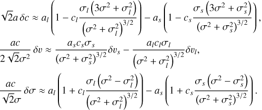 (B.57)
We thus find that, in addition to the velocity variations induced by the photometric effect (proportional to as − al) and the convective blue-shift inhibition effect (υs − υl), changes in the equivalent width csσs − clσl might also affect the velocity. Moreover, we observe that at leading order the contrast variations δc and the FWHM variations δσ are mainly proportional (with negative signs) to the flux variations due to the spot (as − al), with some corrections coming from the shape variations (cs − cl, σs − σl). These indicators might thus be modeled in first approximation with the photometric component of our model if we neglect the correction terms for the shape variations.
Appendix C A computationally efficient GP framework
C.1 Overview of the mean and covariance calculation
To compute the mean function and covariance in an analytical way, be it for the physics-based or data-driven model. In Section 3.4, we made several assumptions reproduced below for convenience
The effect of a single feature is represented as a product of a time window W(t) and a periodic part, decomposed in Fourier series. Denoting by γ = (γW, γper, ϕ0),
 (C.1)
(C.1)
 (C.2)
(C.2)The phase φ0 is distributed uniformly on [0,2π].
The parameters of the window and of the periodic parts are supposed to be statistically independent,
 (C.3)
(C.3)We assume that the properties of the distribution are independent of time, p(γ|η, t) = p(γ|η).
We assume that λ(t) is a stationary random process with expectation µλ(η), and covariance function kλ(τ; η)
The typical timescale of the variation in λ(t) is much greater than the rotation period (2π/ω in Eq. (C.2)).
Based on assumptions 1-6, we can compute the mean and covariance of the process. First, we introduce the following notations for the kernel associated with the window and periodic parts,
 (C.4)
(C.4)
 (C.5)
(C.5)
 (C.6)
(C.6)
 (C.7)
(C.7)
We introduce the average window, its mean and covariance
 (C.8)
(C.8)
 (C.9)
(C.9)
 (C.10)
To establish the final form of the kernels, we proceed by step. We first suppose that λ is constant. Thanks to assumption 1, 2 and 4, as shown in Appendix C.2, Eq. (11) becomes
 (C.11)
And thanks to assumption 3, we can further simplify Eq. (C.11)
 (C.12)
In Appendix C.3, we show that the covariance matrix associated with the kernel  can be put in a semi-separable form, in the particular case where the parameters of the features γ, are fixed. In Appendix C.4, we do the same for the window part. In Appendix C.5, we show that the covariance matrix is still semi-separable when in the case where γ are drawn from the distribution of feature parameters.
If we now take λ(t) as a stationary GP as in assumption 5, as shown in Appendix C.6, the covariance is
 (C.13)
where µi(η) = Eγ(i0(γ)), µj(η) = Eγ(j0(γ)), i0 and j0 are the zero order Fourier coefficient of the periodic part, as defined in Eq. (C.2). Since the timescale of the magnetic cycle is much longer than the magnetic region lifetime (assumption 6), we make the approximation  . Given that the
  kernel has already an amplitude term degenerate with the proportionality coefficient, we simply write
 (C.14)
The first term in Eq. (C.13) is exactly the same as in the case of a constant rate λ = µλ (Eq. (C.12)) but we have an additional term capturing the variations of λ. Similarly, the mean function of the process is
 (C.15)
Finally, in Appendix C.7, we present in detail the data-driven kernels.
C.2 Separation of the window and the periodic components
To simplify the notations, in the reminder of Appendix C, we consider two channels y, z, with associated impulse responses I(t, γ), J(t, γ). We consider here the stationary case, where the rate of spot appearance λ is constant, and the spots properties γ do not depend on time p(γ|η, t) = p(γ|η). The covariance between two time series y(t) = ∑k I(t − tk, γk) and z(t) = ∑k J(t − tk, γk), is
 (C.16)
where η is the set of hyper-parameters describing the spots population properties, I(t, γ) = W(t, γ)i(t, γ) and J(t, γ) = W(t, γ)j(t, γ). Up to now, we did not specify how the time of appearance of the magnetic regions, tk is defined. In the following we define it as the time of maximum "activity" of the spot. This means that W reaches its maximum at t − tk = 0. We assume that the longitude ϕ0 of the spots at t = tk (which is one of the parameters γ) is uniformly distributed in [0,2π] and independent of tk and of the other spots properties. We thus take this parameter out of γ, and rewrite I, J as I(t, ϕ0, γ) = W(t, γ)i(ϕ(t), γ) and J(t, ϕ0, γ) = W(t, γ) j(ϕ(t), γ), with ϕ(t) = ϕ0 + ωt, such that
 (C.17)
We first aim at computing
 (C.18)
In the case I = J, the Fourier transform of k1,I is the power spectral density of I (Wiener–Khinchin theorem)
 (C.19)
In the more general case,
 (C.20)
Moreover, since I is the product of W and i, its Fourier transform is written as a product of convolution
 (C.21)
where ik is the Fourier coefficient
 (C.22)
The same is true for J and the Fourier transform of kI,J is thus written as
 (C.23)
We now integrate this over the longitude at maximum activity ϕ0. This longitude only appears in the term exp(i(l − k)ϕ0), and we have
 (C.24)
thus the integral of  simplifies to
 (C.25)
Finally ky,z simplifies to
 (C.26)
with
 (C.27)
C.3 Efficient modeling with S+LEAF
The kernel of Eq. (B.40) can be very efficiently modeled using S+LEAF (Delisle et al. 2020, 2022) or celerite (Foreman-Mackey et al. 2017). Indeed, in the general case, the cost of likelihood evaluations of a GP is proportional to the number of measurements cubed. For a restricted class of kernel functions, the S+LEAF and celerite GP frameworks allow one to significantly reduce this cost, to a linear scaling with the number of points. In order to be able to use these frameworks, the covariance between the measurements Y = (Y1,…, Yn) must be semiseparable, that is it can be written:
 (C.28)
where r is the rank of the semiseparable representation. In particular, sums and products of exponential kernels, sinusoidal kernels, and Matérn kernels are semiseparable. As shown in Delisle et al. (2022), this reasoning remains valid when considering several time series affected by the same GP but with different coefficients. In this case, the different time series should be merged in a single heterogeneous time series Y, ordered by increasing time, and whose covariance should be semiseparable.
We consider q time series y(1)(t),…, y(q)(t), which we merge and sort by increasing time in a single heterogeneous time series Y. Considering only the periodic part ki,j for a fixed set of spot parameters γ, and ignoring the window part kW for now, the covariance matrix of the merged time series is
 (C.29)
for a > b and where Ik is the index associating with each point in the merged time series Y the identifier of the original time series it comes from and is,k is the k-th Fourier coefficient of the time series s. The covariance of Eq. (C.29) is thus semiseparable with rank r = 2d + 1. However, to obtain Eq. (C.29), we neglected the window part kW, and more importantly, we assumed fixed parameters γ for the spots.
C.4 Window function
Up to now we did not specify the shape W of the spots’ appearing and disappearing process, which models the evolution of the combined effect of area and temperature of the feature as a function of time. In Section 3.1, we mentioned that on the Sun, spots and faculae tend to appear faster than they decay. To have a S+LEAF representation of the noise, in the present work the window function is such that both its increase and decrease in intensity are exponential, potentially with different time-scales.
We provide in Table C.1 the kernel kW obtained when assuming different window shapes W : sudden spot appearing and exponential decay, symmetric or asymmetric exponential appearing and disappearing. In these three cases, the obtained kernel is semiseparable with low rank (see Foreman-Mackey et al. 2017; Delisle et al. 2022). More generally, the Matérn kernel family can be used for efficient modeling of kW with S+LEAF or celerite.
Finally, for fixed spot properties γ, the covariance matrix of the merged time series Y, including the window contribution, is semiseparable with rank r = rWrper.. = rw(2d + 1) since the kernel is the product of two semiseparable kernels (see Eq. (C.26)).
C.5 Distribution of spot properties
We now aim at integrating our kernel over the distribution of spot parameters γ. We assume that the spot parameters γ can be split in two sets of independent parameters, γW (only affecting W) and γper. only affecting the periodic part. By independent we mean
 (C.30)
such that the integral of Eq. (C.26) can be written as
 (C.31)
with
 (C.32)
where kW(τ, γW) and  are given in Eqs. (C.4) and (C.6), respectively.
In the following, we assume that the integral of the window kernel kW(τ; η) can still be approximated with a Matérn kernel, such that it remains semiseparable. For the periodic part,  can be decomposed in a Fourier series, and its k-th coefficient is
 (C.33)
These integral might be performed analytically for some specific choices of distributions p(γ|η). However, this is beyond the scope of this article and we rather turn here to numerical integrals. We thus need to perform an integral for each harmonics k and each couple i, j of original time series (RV and indicators). For each harmonics k we obtain a Hermitian positive definite matrix  of size q × q of these integrated coefficients, where q is the number of original time series. We then compute a square root of the matrix Ck (e.g., by Cholesky decomposition or eigendecomposition)
 (C.34)
such that the coefficients,  , are given by
 (C.35)
With such a decomposition, we obtain a semiseparable representation for  with rank q(2d + 1), where q is the number of considered time series (RV and indicators) and d is the harmonics at which the Fourier series is truncated. Finally, the full covariance matrix – including the window part kW and integrated over the distribution of spots parameters – is semiseparable with rank r = qrW(2d + 1).
We note that the integrals over the distribution of spot parameters required to compute the matrices Ck and Rk might present a significant computational cost. For better performances, we precompute the matrices Rk on a grid of values for η, and then interpolate on this grid to get an estimate of Rk for a given η.
C.6 Variable rate λ
We now consider the case of a variable spot appearance rate λ(t). We assume that λ(t) is a stationary random process with expectation µλ(η), and covariance function kλ(τ; η). Following previous sections, we obtain the following conditional expectations (given λ):
 (C.36)
Moreover, the reasoning of Sects. C.2–C.5 holds and we have
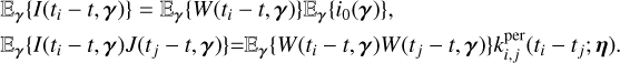 (C.37)
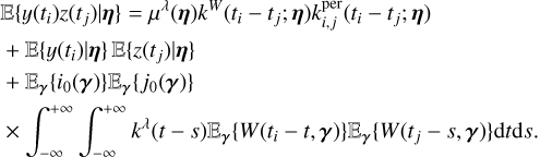 (C.38)
The last line is the convolution product of kλ and the autocorrelation of the mean window function  . This autocorrelation
  differs from the mean autocorrelation kW , since the mean over the spot properties is taken before computing the autocorrelation.
Finally, the kernel function in the case of a variable spot appearance rate is given by
 (C.39)
where µi(η) = Eγ(i0(γ)), µj(η) = Eγ(j0(γ)). The first term in Eq. (C.39) is exactly the same as in the case of a constant rate λ = µλ, but we have an additional term capturing the variations of λ.
Kernels (kW) obtained for different window shapes (W), normalized such that kW(0) = 1.
If we assume that both kλ and  can be approximated by Matérn 1/2 kernels,
 (C.40)
 (C.41)
we obtain
 (C.42)
In the limit  , we have
 (C.43)
which is a Matérn 1/2 kernel with timescale ρλ and amplitude  .
.
Similarly, if kλ and  can be approximated by Gaussian kernels,
 (C.44)
 (C.45)
their convolution is also a Gaussian kernel:
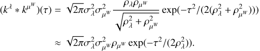 (C.46)
In the limit  , the kernel
  can typically be approximated by a decay kernel with timescale ρλ and with an amplitude scaling as
  .
.
C.7 Data-driven kernels
Replacing Eq. (C.2) in Eq. (11), we showed in Appendix C.5) that
 (C.47)
where
 (C.48)
In the case of a real-valued signal, we show also in Appendix C.5 for a given k, 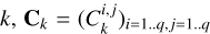 considered as a q × q matrix has a Hermitian symmetry. As a consequence, it can be written with the Cholesky decomposition, as a product of a lower triangular matrix Rk and its complex transpose
  ,
,
 (C.49)
In practice, we need to compute the likelihood within a MCMC or nested sampling algorithm, so we need to evaluate the integrals (C.48) for millions of different values of η. For the physics-based stellar activity model of Section 3, to speed up these evaluations, we pre-compute the integrals as well as Rk(η) in Eq. (C.49) on a tight grid of η parameters, and interpolate linearly for the values of η in the MCMC chain. Another option consists in using the  directly as our hyperparameters η, which we describe below.
To avoid manipulating complex numbers in the numerical implementation, instead of using complex-valued matrices Rk we use as variables their complex and imaginary parts. We denote them by Ak and Bk. Then, from Eq. (C.49),
 (C.50)
Since we focus on real-valued signals, we have  (see Eq. (C.47)). Writing kper(τ; η) the matrix
  , we have
 (C.51)
where  is the term-by-term conjugate of Ck(η) (not its complex transpose). Injecting Eq. (C.49) in Eq. (C.52) yields
 (C.52)
We define our new hyper parameters η = (αk, βk)k=0..d as
 (C.53)
 (C.54)
and we define the MultiFourierKernel function as
 (C.55)
where ak and bk are q × q matrices defined as
 (C.56)
 (C.57)
Because the Rk matrices are lower-triangular complex matrices obtained from Cholesky decomposition, α and β have a form
 (C.58)
 (C.59)
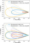 |
Fig. F.1 RV effect as a function of the flux effect. Plain lines correspond to a RV effect only due to the photometric effect only, and dashed line to an RV signal with equal contribution from the photometric and convective blueshift inhibition effects. Top: i = 0 and bottom i = 0.5 rad. Colors are consistent with Fig. 3 |
Appendix F Additional discussions
F.1 Phase shifts might relate to the ratio of spots to faculae
Assuming a constant limb darkening, as is noted in Aigrain et al. (2012), the RV effect due to the photometric effect (Eq. (13)) is proportional to the derivative of the inhibition of convective blueshift effect (Eq. (14)). We can write that RV impulse response g, as ɡ(t + τ) = ɡcb(t) + ɡ′cb(t)τ and ɡ′cb(t) = αɡph(t). This is just another way to rewrite the FF′ approximation of Aigrain et al. (2012), and this is valid only if the limb-darkening effect is the same for the RV photometric effect, and the convective blueshift inhibition RV effect. This is incorrect, in particular because plages have a limb-brightening effect (Meunier et al. 2010a). Nonetheless, we lay out the reasoning with the assumption that the limb darkening is constant as a starting point for a more realistic model.
The opposite of the flux impulse response in Eq. (15), as apparent in Fig. 3 is in phase with the inhibition of the convective blueshift. As long as the RV photometric effect is smaller than the inhibition of convective blueshift by a factor 3 – 4, we can make the approximation
 (F.1)
(F.1)
The absolute value of the phase shift depends on several parameters. Its sign is more robustly defined by the ratio of spots to faculae through the sign of ΔF. In any case, ΔVcb is positive because redshifts are positive, and ΔF is small compared to F. If ΔF is negative, then τ is positive.
We expect that the log R′HK effect in RV is approximately proportional to the projected area of the magnetic region. As a result, it behaves approximately proportionally to the flux. If the magnetic region is bright, then RV should be late compared to photometry and if the region is dark, RV is in advance compared to the log R′HK. In Hara et al. (2022), we showed that in the HARPS-N RV observations of the Sun (Dumusque et al. 2021), RV is consistently in advance of 20 ± 6°, which supports that the RV photometric effect is dominated by spots on the Sun.
F.2 Building relevant indicators
As mentioned in Section 2.4, we could try to find a spectral variability indicator such that the impulse response of a stellar feature h(t, γ) in this indicator is such that the effect of the feature on the signal of interest (photometry or RV), ɡ(t, γ), is proportional to h(t, γ) for all γ. However, in most cases indicators do not exhibit a linear relationship. It is known that RV and photometry, or RV and indicators might exhibit a so-called closed-loop relations (Bonfils et al. 2007; Forveille et al. 2009; Santerne et al. 2015; Lanza et al. 2018; Collier Cameron et al. 2019; Zhao et al. 2024). This means that when one is plotted against the other, the figure seems to close on itself. In Fig. F.1, we show the behavior of RV versus photometry when they are modeled as in Sec 3.1.
Another approach would be to build several indicators, such that the impulse response of stellar features in the signal of interest is a linear combination of the responses in the different channels. In Haywood et al. (2022), it is argued that the unsigned magnetic flux is a good proxy for the RV component due to the inhibition of the convective blueshift. Neglecting the limb-darkening effect, the radial magnetic field projected onto the line of sight is proportional to RV convective blueshift effect. Since this one dominates on the Sun, we expect it to be a good indicator. However, the limb-darkening law might differ for the velocity and the magnetic field might differ, so we do not expect the correlation to be exact.
F.3 Link with Doppler imaging
Our framework could be extended to perform more classical Doppler imaging. Luger et al. (2021a) map linearly the stellar surface brightness developed in spherical harmonics to the spectrum. In Lehmann & Donati (2022), the authors map the time series of LSD onto principal components, which can be seen as a data-driven way to retrieve the spherical harmonics. By defining observation channels as the spectrum projected on a basis corresponding to the spherical harmonics, we could obtain an estimate of the evolution of their coefficient with time.
References
- Ahrer, E., Queloz, D., Rajpaul, V. M., et al. 2021, MNRAS, 503, 1248 [NASA ADS] [CrossRef] [Google Scholar]
- Aigrain, S., Pont, F., & Zucker, S. 2012, MNRAS, 419, 3147 [NASA ADS] [CrossRef] [Google Scholar]
- Berdyugina, S. V., & Usoskin, I. G. 2003, A&A, 405, 1121 [NASA ADS] [CrossRef] [EDP Sciences] [Google Scholar]
- Bloomfield, P. 2004, Fourier Analysis of Time Series: An Introduction, Fourier Analysis of Time Series: An Introduction (Hoboken: Wiley) [Google Scholar]
- Boisse, I., Bonfils, X., & Santos, N. C. 2012, A&A, 545, A109 [NASA ADS] [CrossRef] [EDP Sciences] [Google Scholar]
- Bonfils, X., Mayor, M., Delfosse, X., et al. 2007, A&A, 474, 293 [NASA ADS] [CrossRef] [EDP Sciences] [Google Scholar]
- Borgniet, S., Meunier, N., & Lagrange, A. M. 2015, A&A, 581, A133 [NASA ADS] [CrossRef] [EDP Sciences] [Google Scholar]
- Camacho, J. D., Faria, J. P., & Viana, P. T. P. 2023, MNRAS, 519, 5439 [NASA ADS] [CrossRef] [Google Scholar]
- Cegla, H. 2019, Geosciences, 9, 114 [NASA ADS] [CrossRef] [Google Scholar]
- Collier Cameron, A., Mortier, A., Phillips, D., et al. 2019, MNRAS, 487, 1082 [Google Scholar]
- Crass, J., Gaudi, B. S., Leifer, S., et al. 2021, arXiv e-prints [arXiv:2107.14291] [Google Scholar]
- Delisle, J.-B., Ségransan, D., Dumusque, X., et al. 2018, A&A, 614, A133 [NASA ADS] [CrossRef] [EDP Sciences] [Google Scholar]
- Delisle, J. B., Hara, N., & Ségransan, D. 2020, A&A, 638, A95 [EDP Sciences] [Google Scholar]
- Delisle, J. B., Unger, N., Hara, N. C., & Ségransan, D. 2022, A&A, 659, A182 [NASA ADS] [CrossRef] [EDP Sciences] [Google Scholar]
- Desort, M., Lagrange, A. M., Galland, F., Udry, S., & Mayor, M. 2007, A&A, 473, 983 [CrossRef] [EDP Sciences] [Google Scholar]
- Deutsch, A. J. 1958, in Electromagnetic Phenomena in Cosmical Physics, ed. B. Lehnert (Cambridge: Cambridge University Press), 6, 209 [NASA ADS] [Google Scholar]
- Donati, J. F., Semel, M., Carter, B. D., Rees, D. E., & Collier Cameron, A. 1997, MNRAS, 291, 658 [Google Scholar]
- Dravins, D., Lindegren, L., & Nordlund, A. 1981, A&A, 96, 345 [NASA ADS] [Google Scholar]
- Dumusque, X. 2014, ApJ, 796, 133 [NASA ADS] [CrossRef] [Google Scholar]
- Dumusque, X., Boisse, I., & Santos, N. C. 2014, ApJ, 796, 132 [NASA ADS] [CrossRef] [Google Scholar]
- Dumusque, X., Cretignier, M., Sosnowska, D., et al. 2021, A&A, 648, A103 [NASA ADS] [CrossRef] [EDP Sciences] [Google Scholar]
- Eastman, J. D., Rodriguez, J. E., Agol, E., et al. 2019, arXiv e-prints [arXiv:1907.09480] [Google Scholar]
- Foreman-Mackey, D., Agol, E., Ambikasaran, S., & Angus, R. 2017, AJ, 154, 220 [Google Scholar]
- Fortune, M., Gibson, N. P., Foreman-Mackey, D., et al. 2024, A&A, 686, A89 [NASA ADS] [CrossRef] [EDP Sciences] [Google Scholar]
- Forveille, T., Bonfils, X., Delfosse, X., et al. 2009, A&A, 493, 645 [NASA ADS] [CrossRef] [EDP Sciences] [Google Scholar]
- Frazier, E. N. 1971, Sol. Phys., 21, 42 [Google Scholar]
- Gibson, N. P., Aigrain, S., Roberts, S., et al. 2012, MNRAS, 419, 2683 [NASA ADS] [CrossRef] [Google Scholar]
- Gilbertson, C., Ford, E. B., Jones, D. E., & Stenning, D. C. 2020, ApJ, 905, 155 [Google Scholar]
- Goncharskii, A. V., Stepanov, V. V., Kokhlova, V. L., & Yagola, A. G. 1977, Sov. Astron. Lett., 3, 147 [NASA ADS] [Google Scholar]
- Goncharskii, A. V., Stepanov, V. V., Khokhlova, V. L., & Yagola, A. G. 1982, Soviet Ast., 26, 690 [Google Scholar]
- Gordon, T. A., Agol, E., & Foreman-Mackey, D. 2020, AJ, 160, 240 [NASA ADS] [CrossRef] [Google Scholar]
- Gray, D. F. 2005, The Observation and Analysis of Stellar Photospheres (Cambridge: Cambridge University Press) [Google Scholar]
- Hara, N. C., & Ford, E. B. 2023, Ann. Rev. Stat. Its Appl., 10, 623 [Google Scholar]
- Hara, N. C., Delisle, J.-B., Unger, N., & Dumusque, X. 2022, A&A, 658, A177 [NASA ADS] [CrossRef] [EDP Sciences] [Google Scholar]
- Haywood, R. D., Collier Cameron, A., Queloz, D., et al. 2014, MNRAS, 443, 2517 [Google Scholar]
- Haywood, R. D., Milbourne, T. W., Saar, S. H., et al. 2022, ApJ, 935, 6 [NASA ADS] [CrossRef] [Google Scholar]
- Howard, R. F. 1992, Sol. Phys., 137, 51 [Google Scholar]
- Javaraiah, J. 2011, Sol. Phys., 270, 463 [NASA ADS] [CrossRef] [Google Scholar]
- Jones, D. E., Stenning, D. C., Ford, E. B., et al. 2022, arXiv e-prints [arXiv:1711.01318] [Google Scholar]
- Khokhlova, V. L. 1976, Astron. Nachr., 297, 203 [Google Scholar]
- Klein, B., Aigrain, S., Cretignier, M., et al. 2024, MNRAS, 531, 4238 [Google Scholar]
- Kochukhov, O. 2016, in Lecture Notes in Physics, eds. J.-P. Rozelot, & C. Neiner (Berlin: Springer Verlag), 914, 177 [Google Scholar]
- Kopp, G. 2020, SORCE Level 3 Total Solar Irradiance Daily Means V019, Greenbelt, MD, USA, Goddard Earth Sciences Data and Information Services Center (GES DISC), accessed: 2023-01-10 [Google Scholar]
- Korhonen, H., Berdyugina, S. V., Strassmeier, K. G., & Tuominen, I. 2001, A&A, 379, L30 [NASA ADS] [CrossRef] [EDP Sciences] [Google Scholar]
- Lanza, A. F., Malavolta, L., Benatti, S., et al. 2018, A&A, 616, A155 [NASA ADS] [CrossRef] [EDP Sciences] [Google Scholar]
- Lefebvre, M., & Bensalma, F. 2015, Appl. Math. Modell., 39, 230 [Google Scholar]
- Lehmann, L. T., & Donati, J. F. 2022, MNRAS, 514, 2333 [CrossRef] [Google Scholar]
- Livingston, W. C. 2002, Sun, ed. A. N. Cox (New York, NY: Springer New York), 339 [Google Scholar]
- Lovis, C., & Fischer, D. 2010, Exoplanets, Radial Velocity Techniques for Exoplanets (Tucson, AZ: University of Arizona Press), 27 [Google Scholar]
- Luger, R., Foreman-Mackey, D., & Hedges, C. 2021a, AJ, 162, 124 [NASA ADS] [CrossRef] [Google Scholar]
- Luger, R., Foreman-Mackey, D., Hedges, C., & Hogg, D. W. 2021b, AJ, 162, 123 [NASA ADS] [CrossRef] [Google Scholar]
- Mandal, S., Karak, B. B., & Banerjee, D. 2017, ApJ, 851, 70 [Google Scholar]
- Martinez Pillet, V., Moreno-Insertis, F., & Vazquez, M. 1993, A&A, 274, 521 [Google Scholar]
- Mayor, M., Lovis, C., & Santos, N. C. 2014, Nature, 513, 328 [Google Scholar]
- Mendel, J. M. 1991, Proceedings of the IEEE, 79, 278 [Google Scholar]
- Meunier, N. 2023, in Exoplanets, Star-Planet Interactions, eds. L. Bigot, J. Bouvier, Y. Lebreton, A. Chiavassa, & A. Lèbre (Tucson: University of Arizona Press), 22 [Google Scholar]
- Meunier, N., & Lagrange, A. M. 2019a, A&A, 628, A125 [NASA ADS] [CrossRef] [EDP Sciences] [Google Scholar]
- Meunier, N., & Lagrange, A. M. 2019b, A&A, 629, A42 [NASA ADS] [CrossRef] [EDP Sciences] [Google Scholar]
- Meunier, N., Desort, M., & Lagrange, A.-M. 2010a, A&A, 512, A39 [NASA ADS] [CrossRef] [EDP Sciences] [Google Scholar]
- Meunier, N., Lagrange, A. M., & Desort, M. 2010b, A&A, 519, A66 [NASA ADS] [CrossRef] [EDP Sciences] [Google Scholar]
- Meunier, N., Lagrange, A. M., Boulet, T., & Borgniet, S. 2019, A&A, 627, A56 [NASA ADS] [CrossRef] [EDP Sciences] [Google Scholar]
- Meyer, F., Schmidt, H. U., Weiss, N. O., & Wilson, P. R. 1974, MNRAS, 169, 35 [Google Scholar]
- Nèmec, N. E., Shapiro, A. I., Isik, E., et al. 2022, ApJ, 934, L23 [CrossRef] [Google Scholar]
- Petit, P., Donati, J. F., Hébrard, E., et al. 2015, A&A, 584, A84 [NASA ADS] [CrossRef] [EDP Sciences] [Google Scholar]
- Piskunov, N. E., & Rice, J. B. 1993, PASP, 105, 1415 [NASA ADS] [CrossRef] [Google Scholar]
- Rajpaul, V., Aigrain, S., Osborne, M. A., Reece, S., & Roberts, S. 2015, MNRAS, 452, 2269 [Google Scholar]
- Rasmussen, C. E., & Williams, C. K. I. 2005, Gaussian Processes for Machine Learning (Adaptive Computation and Machine Learning) (Cambridge: The MIT Press) [Google Scholar]
- Rice, J. B., & Strassmeier, K. G. 2000, A&AS, 147, 151 [NASA ADS] [CrossRef] [EDP Sciences] [Google Scholar]
- Rincon, F., & Rieutord, M. 2018, Liv. Rev. Sol. Phys., 15, 6 [Google Scholar]
- Saar, S. H., & Donahue, R. A. 1997, ApJ, 485, 319 [Google Scholar]
- Santerne, A., Díaz, R. F., Almenara, J.-M., et al. 2015, MNRAS, 451, 2337 [NASA ADS] [CrossRef] [Google Scholar]
- Schrijver, C. J. 2002, Astron. Nachr., 323, 157 [Google Scholar]
- Shapiro, A. I., Solanki, S. K., Krivova, N. A., Yeo, K. L., & Schmutz, W. K. 2016, A&A, 589, A46 [NASA ADS] [CrossRef] [EDP Sciences] [Google Scholar]
- Song, A., Zhang, Q., Wang, Y., et al. 2024, A&A, 682, A87 [NASA ADS] [CrossRef] [EDP Sciences] [Google Scholar]
- Strassmeier, K. G. 2009, A&ARv, 17, 251 [Google Scholar]
- Suárez Mascareño, A., Damasso, M., Lodieu, N., et al. 2021, Nat. Astron., 6, 232 [Google Scholar]
- Sulis, S., Lendl, M., Hofmeister, S., et al. 2020, A&A, 636, A70 [NASA ADS] [CrossRef] [EDP Sciences] [Google Scholar]
- Tran, Q. H., Bedell, M., Foreman-Mackey, D., & Luger, R. 2023, ApJ, 950, 162 [CrossRef] [Google Scholar]
- Unruh, Y. C., Solanki, S. K., & Fligge, M. 1999, A&A, 345, 635 [NASA ADS] [Google Scholar]
- Vogt, S. S., & Penrod, G. D. 1983, PASP, 95, 565 [NASA ADS] [CrossRef] [Google Scholar]
- Vogt, S. S., Penrod, G. D., & Hatzes, A. P. 1987, ApJ, 321, 496 [Google Scholar]
- Xu, J. C., Xie, J. L., & Qu, Z. N. 2017, ApJ, 851, 141 [Google Scholar]
- Yu, H., Aigrain, S., Klein, B., et al. 2024, MNRAS, 535, 634 [Google Scholar]
- Zhao, L. L., Bedell, M., Hogg, D. W., & Luger, R. 2024, ApJ, 977, 140 [Google Scholar]
The documentation can be accessed at https://obswww.unige.ch/~delisle/spleaf/doc/index.html#examples
Downloaded from https://lasp.colorado.edu/lisird/data/sorce_tsi_24hr_l3
The documentation is accessible at this address https://obswww.unige.ch/~delisle/spleaf/doc/index.html#examples, and the source code at https://gitlab.unige.ch/jean-baptiste.delisle/spleaf.
All Tables
Set of parameters explored in the MCMC of the lat. dist. run, with their priors and posteriors (median and 68.27% interval).
Set of parameters explored in the MCMC of the opp. lat. run, with their priors and posteriors (median and 68.27% interval).
Cross-validation tests for the active-regions component of the model trained on Sun RV + photometry.
Cross-validation tests for the active-regions component of the model trained on Sun RV and various activity indicators.
Kernels (kW) obtained for different window shapes (W), normalized such that kW(0) = 1.
All Figures
|
Fig. 1 (a) Inouye Solar Wave Front Correction (WFC) image, captured on Jan. 28, 2020, at 789 nm. The granulated structures around the spot are due to convection: hot plasma moves upward at the center of granules, cools down, and goes downwards between granules (darker intergranular regions). The contribution of brighter intra-granular regions exceeds that of intergranular ones, creating a so-called convective blueshift on observed spectra. Credit: NSO/AURA/NSF. (b) SDO observation of the Sun at wavelength 1700 Å. The bright regions are called faculae, and the dark regions are called spots. Both faculae and spots inhibit the upward convective motion of the gas (Dravins et al. 1981). Faculae cover more area than spots, but have a smaller temperature contrast with the quiet surface. The latitude, number, and lifetime of the spots varies along stellar magnetic cycles, on the timescale of a few years (11 years for the Sun). Courtesy of NASA/SDO and the AIA, EVE, and HMI science teams. (c) Group of sunspots observed at two different dates, top: January 6, 2012, bottom: January 8, 2012. Courtesy of NASA/SDO. |
| In the text | |
|
Fig. 2 Viewing geometry: a stellar feature represented by the dark blue point moves as the star rotates and is visible only a fraction of the time. It modifies the local emission, and velocity of the plasma, which appears to move outwards because of its convective motion. We parametrize the position of the feature with the angle between the sky plane and rotation axis, |
| In the text | |
|
Fig. 3 In (a) and (c), colored lines represent the path of dark spots as the star rotates at different latitudes. In (a), the rotation axis in the plane of the sky, in (c) the rotation axis is tilted by 0.5 rad towards the observer with respect to the sky plane. (b1)/(d1): effect on RV of the imbalance break between the approaching an receding limb (ɡph in Eq. (13)), (b2)/(d2): RV convective blueshift inhibition effect on RV (ɡcb in Eq. (14)), (b3)/(d3): effect on photometry of the stellar surface darkening (h in Eq. (15)). |
| In the text | |
|
Fig. 4 Different RV effects of an equatorial dark spot due to the photometric effect (a) and inhibition of the convective blueshift (b), with limb-darkening laws of different degrees (simply l(µ) = µ,µ2,µ3). With the notations of Eq. (17), in increasingly darker yellow we take d = 0,1,2,3 and for j < d, aj = 0. |
| In the text | |
|
Fig. 5 RV convective blueshift inhibition on the RVs as a function of the rotation phase with a rising and decaying amplitude with a star inclined as in Fig. 3d. Black line: window function consisting of two exponentials, thin lines: effect of a spot without amplitude variation, bold lines: effect of the spot with varying amplitude. Colors correspond to the effect of spots at different latitudes (color code is the same as Fig. 3d). In (a) the maximum amplitude of the spot is attained on the visible hemisphere at the longitude of the observer (ϕ0 = 0), and in (b) the maximum amplitude is attained when the spot is 180° away from the observer. The window is chosen to reproduce the fact that, on the Sun, spots appear 10-11 times faster than they vanish (Howard 1992; Javaraiah 2011). |
| In the text | |
|
Fig. 6 Simulated RV as a function of time when the RV effect is due to a combination of inhibition of convective blueshift and a RV photometric effect. The average lifetime of the magnetic regions is 15 days. The rate varies as a A/2(1 + cos 2πt/Pmaɡc) where Pmaɡc = 11 years and A is such that there are on average 50 spots visible each day. |
| In the text | |
|
Fig. 7 Illustration of the photometric effect of spots, plages, and global effect of an active region accounting for the limb-brightening effect, the limb-darkening effect, and the projection effect. |
| In the text | |
|
Fig. 8 Corner plot of the MCMC samples of the lat. dist. run for the Sun’s inclination and the spots latitude distribution parameters. The dashed lines correspond to the priors. |
| In the text | |
|
Fig. 9 Corner plot of the MCMC samples of the opp. lat. run for the Sun’s inclination and the spots latitude distribution parameters. The dashed lines correspond to the priors. |
| In the text | |
|
Fig. 10 Kernel function using the maximum a posteriori parameters from the MCMC of the lat. dist. run. |
| In the text | |
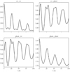 |
Fig. 11 Same as Fig. 10 but zoomed on the range 0–100 d. |
| In the text | |
|
Fig. 12 Maximum a posteriori solution of the lat. dist. run superimposed over the RV (top) and photometric (bottom) data. |
| In the text | |
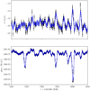 |
Fig. 13 Same as Fig. 12 but zoomed on a few solar rotation periods. |
| In the text | |
|
Fig. 14 Maximum a posteriori solution of the best (in terms of crossvalidation score) data-driven FENRIR model superimposed over the RV (top), FWHM (middle), and BIS (bottom) data, zoomed on a few rotation period. The train set is highlighted with black points, while the test set is highlighted with red points. |
| In the text | |
|
Fig. 15 Histogram of RVs simulated with a FENRIR process, with a rate of λ = 1.2 and λ = 0.2 magnetic region appearing per day (respectively the blue and orange histograms). |
| In the text | |
|
Fig. 16 Histogram of normalized RVs simulated with a FENRIR process, with a rate of λ = 1.2 and λ = 0.2 magnetic region appearing per day (respectively the blue and orange histograms). RVs are normalized by subtracting the mean of the time-series and dividing by its empirical standard deviation. The black line represents a Gaussian distribution with vanishing mean and variance 1. |
| In the text | |
|
Fig. 17 Yellow histogram: Histogram of RVs measured on the Sun (public data Dumusque et al. 2021) by HARPS-N after binning by 15 hours, and fitting and subtracting a 9-th order polynomial. The solid yellow curve is a Gaussian ditribution with the same mean and variance as the data. |
| In the text | |
|
Fig. 18 Absolute value of the bispectrum divided by an upper bound on its mean squared error, for a purely periodic, equatorial spot signal with a contribution of the convective blueshift inhibition twice that of the RV photometric effect, and |
| In the text | |
|
Fig. 19 (a): Real part of Eq. (48), ω, ω coefficient as a function of stellar inclination |
| In the text | |
|
Fig. F.1 RV effect as a function of the flux effect. Plain lines correspond to a RV effect only due to the photometric effect only, and dashed line to an RV signal with equal contribution from the photometric and convective blueshift inhibition effects. Top: i = 0 and bottom i = 0.5 rad. Colors are consistent with Fig. 3 |
| In the text | |
Current usage metrics show cumulative count of Article Views (full-text article views including HTML views, PDF and ePub downloads, according to the available data) and Abstracts Views on Vision4Press platform.
Data correspond to usage on the plateform after 2015. The current usage metrics is available 48-96 hours after online publication and is updated daily on week days.
Initial download of the metrics may take a while.