© The Authors 2025

1 Introduction

Space missions, for which rendezvous with Solar System bodies and sometimes landing demand the highest possible accuracy in the navigation of spacecraft, also require increased accuracy in the ephemerides of the targeted body(ies). It is therefore necessary to model as well as possible all forces acting on these bodies, which may include improvements in the orbit of natural satellites such as Phobos in the case of the Martian Moons eXploration (MMX) mission (Kuramoto et al. 2022). Among the model uncertainties are those related to coupling between the complex shapes, and gravitational attractions of a satellite and its parent planet. The Mars-Phobos case was studied analytically by Borderies and Yoder (Borderies & Yoder 1990), especially in relation to Phobos libration, taking into account the satellite gravity harmonic coefficients to the degree and order two. Jacobson and Lainey (Jacobson & Lainey 2014), and more recently Yang et al. (Yang et al. 2024), have also studied this problem, but without the coupling terms (CoT) between Mars and Phobos. Our goal has been to revisit the general expression of the mutual gravitational field of two bodies, and first to apply it and quantify the orbital effects on the Didymos–Dimorphos system, which is unusual in terms of shape and relative distance. Then, we numerically assess the effect of the full gravitational CoT on the Phobos orbit with respect to other small perturbations such as the tidal forces. In this paper, we neither work out the dynamical equations for the rotational (attitude) dynamics of the bodies involved, nor do we propagate those dynamics.

2 General formulation

The mutual gravitational potential of two bodies (B) and (B’) is a function, U, which simply depends on the shape and mass distribution of both bodies interacting on each other. Its general expression is $$U=G{\displaystyle {\iiint }_B{\displaystyle {\iiint }_{B^{\prime }}\frac{d{\mu }_{P}d{\mu }_{P\prime }}{PP\prime }}},$$(1)

where G is the Newtonian gravitational constant, and dµ_P and dµ′_P are the infinitesimal mass densities of the two bodies at any couple of points, P, P′. As is usual in celestial mechanics, we note that U is a force potential function (the opposite of the potential energy).

For a single body, its gravitational potential is usually represented as a (truncated) spherical harmonics series in a reference frame, [R], fixed relative to it. At any point of spherical coordinates, r, ϕ, λ (radius vector, latitude, longitude), the body gravitational potential can be written as (Balmino & Borderies 1978; Balmino 1994) $$U(r,\varphi ,\lambda )=\frac{GM}{r}{\displaystyle \sum _{l=0}^{\infty }{\left(\frac{R}{r}\right)}^l}{\displaystyle \sum _{m=-l}^l{K}_{lm}}{Y}_{lm}(\varphi ,\lambda ),$$(2)

where M is the mass of the body, G is the Newton constant, and R is a reference equatorial radius. K_lm are the complex gravitational harmonics coefficients of degree l and order m, and Y_lm the corresponding complex harmonics functions with the following definition: $$Y_{lm}(\varphi ,\lambda )=P_{lm}(\sin \varphi )e^{\text{i}m\lambda },$$(3)

where P_lm (m > 0) is the usual Legendre associated function, extended to negative orders by $$P_{l,-m}(u)={(-1)}^m\frac{(l-m)!}{(l+m)!}{P}_{lm}(u).$$(4)

The complex K_lm coefficients are related to the usual real coefficients, C_lm and S_lm (m > 0), by $$\left(2-{\delta }_{0m}\right)K_{lm}=C_{lm}-\text{i\hspace{0.17em}}{S}_{lm},$$(5)

where δ_0m is the Dirac delta (equal to 1 if m = 0 and 0 else), $$\left(2-{\delta }_{0m}\right)K_{l,-m}=\left(C_{lm}+\text{i}{S}_{lm}\right)\frac{(l+m)!}{(l-m)!}{(-1)}^m.$$(6)

In the following, we use non-normalized functions and coefficients, which is appropriate from a numerical point of view, since we do not go to a high degree and order in this work.

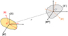Fig. 1 Two bodies, (B) and (B′), and their body-fixed reference systems, [R] and [R′], respectively. [R0] and [R′0] are two other reference frames that have the same orientation in space.

2.1 Mutual potential

For two bodies, (B) and (B′), we considered reference frames [R⁰] for (B) and [R′⁰] for (B′), whose origins, O, O′, are distant from r and whose axes have the same orientations (Fig. 1).

We let $K_{lm}^0$ and $K_{pk}^{\prime 0}$ be the complex gravity harmonics of (B) and (B′) in the reference frames [R⁰] and [R′⁰], respectively. The mutual gravitational potential can be expanded as (Borderies 1978) $$\begin{array}{l}U(r,\delta ,\alpha )=\frac{GM{M}^{\prime }}{r}{\displaystyle \sum _{l=0}^{\infty }{\left(\frac{R}{r}\right)}^l}{\displaystyle \sum _{m=-l}^l\frac{K_{lm}^0}{(l-m)!}}{\displaystyle \sum _{p=0}^{\infty }{(-1)}^p}{\left(\frac{R^{\prime }}{r}\right)}^p\\ {\displaystyle \sum _{k=-p}^p\frac{K_{pk}^{\prime 0}}{(p-k)!}}(l+p-m-k)!Y_{l+p,m+k}(\delta ,\alpha ),\end{array}$$(7)

where M′, and R′ are, for (B′), analogous to M and R, and α and δ are, respectively, the right ascension and declination of O′ in [R⁰]. In this formula, we can identify certain terms that correspond to usual simplifications. In order to distinguish them, we shall refer to them in the remainder of this article using the conventions of Table 1.

For calculation purposes, we must refer the $K_{lm}^0$ coefficients of (B) to its harmonics, K_jn, in its proper body fixed system, [R], and also refer the $K_{pk}^{\prime 0}$ coefficients of (B') to its harmonics, $K_{qs}^{\prime 0}$, in its body fixed system, [R']. To do so, we introduced the Euler angles, Ψ, Θ, Φ, of [R] with respect to [R⁰], as is defined in Fig. 2, and similarly the “3-1-3” Euler angles, Ψ′, Θ′, Φ′, of [R′] with respect to [R′⁰].

We used the spherical harmonics rotation theorem (Wigner & Fano 1960) in its dual form, which yields $$K_{lm}^0={\displaystyle \text{∑}_{n=\text{−}l}^l{K}_{ln}}\frac{(l+n)!}{(l+m)!}{E}_{lm}^{n*}(\text{Ψ},\text{Θ},\text{Φ}),$$(8)

and $$K_{pk}^{\text{′}0}={\displaystyle \sum _{s=-p}^p{K}_{ps}^{\prime }}\frac{(p+s)!}{(p+k)!}{E}_{pk}^{s*}\left({\text{Ψ}}^{\prime },{\text{Θ}}^{\prime },{\text{Φ}}^{\prime }\right),$$(9)

with $$E_{lm}^n(\text{Ψ},\text{Θ},\text{Φ})={(-1)}^{l-m}{e}^{\frac{\text{i}(n-m)\text{π}}{2}}{e}^{\text{i}(m\Psi +n\text{Φ})}{\text{ℭ}}_{lm}^n(\text{Θ}),$$(10)

where $$\begin{array}{l}{\text{ℭ}}_{lm}^n(\text{Θ})={\displaystyle \sum _{j=\sup (0,-m-n)}^{\inf (l-m,l-n)}{(-1)}^j}{C}_{l-m}^j{C}_{l+m}^{m+n+j}\\ \times {\left(\cos \frac{\text{Θ}}{2}\right)}^{2j+m+n}{\left(\sin \frac{\text{Θ}}{2}\right)}^{2l-2j-m-n}\end{array}$$(11)

are the Clifford polynomials. The conjugate of the $E_{lm}^n$ functions that enter in Eqs. (8) and (9) verify that $$E_{lm}^{n*}={(-1)}^{m+n}{E}_{l,-m}^{-n}.$$(12)

In formulas (8) and (9), we note that the degree of the spherical harmonics is preserved. For comparison purposes with other simplified expressions of U found in the literature, we give in the appendix formulas for the case in which spherical harmonics are limited to the degree and order two for each body and when Ψ = Ψ′ = Θ = Θ′ = 0.

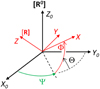Fig. 2 Going from reference system [R0] to another one, [R], by means of the Euler angles, Ψ, Θ, and Φ.

2.2 Dynamical equations

The motion of O′ relative to O is described by the equation $$\overrightarrow{\text{Γ}}\left(O^{\prime }/\left[{\text{R}}^0\right]\right)=\frac{d^2}{d{t}^2}\left(\overrightarrow{O{O}^{\prime }}\right)=\frac{M+M^{\prime }}{M{M}^{\prime }}{\overrightarrow{\nabla }}_{O^{\prime }}U.$$(13)

Then we have to compute the components of the mutual gravitational potential gradient U defined in Eq. (7). X_s being the components of $\overrightarrow{O{O}^{\prime }}$ in [R⁰], these gradient components are $f_{nj,s}=\frac{\partial f_{nj}}{\partial X_s}$, where f_nj is defined ∀n ∊ 〚1, l_max + p_max〛 and ∀ j ∊ 〚−n, n〛 by the equation: $$f_{nj}=r^{-n-1}{Y}_{nj}=r^{-n-1}{P}_{nj}(\sin \delta )e^{\text{i}j\alpha }.$$(14)

These terms originate from formula (7), where n = l + p and j = m + k. It should be noted that the coefficients of such terms capture all of the dependence on the attitudes of both bodies and have no dependence on the relative position of the bodies, in a separable fashion. We followed an approach whereby we wrote P_nj(sin δ) = cos^j δ H_nj(sin δ), H_nj being the Helmholtz polynomials, here non-normalized (the degree and order remain small, as was said above). They were computed by recursive formulas with a fixed order, j, as well as their derivatives. Introducing the direction cosines (ε₁, ε₂, ε₃) of $\overrightarrow{O{O}^{\prime }}$ in [R⁰], we have for j > 0: $$f_{nj}=\frac{1}{r^{n+1}}{H}_{nj}\left({\epsilon }_3\right){\left({\epsilon }_1+\text{i}{\epsilon }_2\right)}^j,$$(15) $$f_{n,-j}={(-1)}^j\frac{(n-j)!}{(n+j)!}{f}_{nj}^{*},$$(16)

from which nonsingular expressions (valid when cos δ = 0) for f_nj,s can be derived (Balmino et al. 1990).

3 Example: Didymos and Dimorphos

We present a simplified case of the Didymos and Dimorphos binary, which was visited by the DART mission (Daly et al. 2023) and which is targeted by the Hera mission (ESA 2022). This example consists of taking the known physical parameters of this binary system, propagating a Keplerian orbit of Dimorphos around Didymos, and evaluating over one revolution the value of the different terms of the acceleration induced by the mutual potential – according to definitions in Table 1.

3.1 Data assumptions

As the precise shape of each of these bodies is not precisely known, we carried out the calculation using ellipsoidal models with the parameters given in Table 2 (Daly et al. 2023); the semimajor axes are those in the X, Y, Z directions of the [R] system for Didymos and similarly in the [R′] system for Dimorphos. For each body, defining: p = a² − b², q = c² − (a² + b²)/2, one can compute the nonzero gravity spherical harmonics according to (Balmino 1994; Boyce 1997) $$\begin{array}{l}{K}_{2l,2m}=\frac{3}{{\text{a}}^{2l}}\frac{l!(2l-2m)!}{2^{2m}(2l+3)(2l+1)!}\\ {\displaystyle \sum _{i=0}^{[(l-m)/2]}\frac{p^{m+2i}{q}^{l-m-2i}}{{16}^{i}i!(m+i)!(l-m-2i)!}},\end{array}$$(17)

where the a^2l term corresponds to a scaling factor (Brillouin sphere radius) equal to a. The resulting coefficients (unnormalized) are given up to the degree and order six in Table 3 for the two bodies.

The mean orbital parameters used in the computation are listed in Table 4. Finally, we fixed the Euler angles (rotational elements) at the following values: $$\begin{array}{l}\text{Ψ}={\text{Ψ′}}^{}=\text{Θ}={\text{Θ}}^{\prime }=0\hfill \\ {\text{Φ}}_{\text{Didymos }}=t\text{∗}360/{(2.2593\text{∗}3600)}^{\circ }\hfill \\ {\text{Φ}}_{\text{Dimorphos }}=t\ast 360/{(11.9217\text{∗}3600)}^{\text{∘}},\hfill \end{array}$$

where 360/(11.9217 * 3600) is the mean motion (n) of Dimorphos (before the DART impact) and t is the time in seconds.

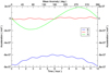Fig. 3 Acceleration magnitudes of Dimorphos over one orbit for the direct term (DT).

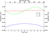Fig. 4 Acceleration magnitudes of Dimorphos over one orbit for IT.

3.2 Numerical results

The maximum and minimum accelerations along one orbit are given in Table 5 for the different classes of terms: central, direct, indirect, and coupling. Indirect accelerations are smaller though close to the direct terms; the CoT amount to about 1% of the direct ones, which is significant for the system dynamics.

Figures 3, 4, and 5 more precisely show the behaviour of the different terms (apart from the central one). In addition to once-per-revolution variations in the direct and indirect radial and normal accelerations, higher-frequency variations due to direct and CoT are clearly visible, especially in the tangential and radial directions; the direct perturbations dominate due to the much higher mass and C₂₀ of Didymos.

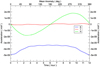Fig. 5 Acceleration magnitudes of Dimorphos over one orbit for CoT.

4 Application to Mars-Phobos

To see the impact of the mutual potential on a well-known orbit, we chose the Mars-Phobos system. Phobos has a rather unusual gravitational configuration with Mars, being relatively close and not spherical in shape.

We focus on the effects of the gravitational CoT compared to other forces at work in the system, the tidal effects of Mars (i.e., the k₂ Love number contribution), the third-body perturbations mainly due to the Sun and Jupiter, and relativistic effects.

4.1 Orbit models and assumptions

4.1.1 Mars and Phobos orientation

For the body orientation and rotation, the models in the IAU 2015 standards (Archinal et al. 2018) were used. For Phobos, the correction (Archinal et al. 2019) has been taken into account in this study, even though its impact remains small.

4.1.2 Gravity model

The Martian gravity model used is the Konopliv model (Konopliv et al. 2016) developed to degree 120. The version used is MRO120d, but only the first eight degrees were retained.

The Phobos gravity model was derived from the transformation of the most accurate body shape (Ernst et al. 2023) into gravitational spherical harmonics under the assumption of uniform mass distribution. This model is given in Appendix B. We assumed a GM value of 708 700 m³/s² (consistent with Jacobson & Lainey 2014) and a translation was done to make the center of mass, O, and the center of figure, C, coincide. Thanks to this translation, $\overrightarrow{OC}$, of (82.194, 521.606, 31.433) (m), the degree one coefficients vanish.

4.1.3 Other forces

Third body and tidal forces were taken into account in accordance with current knowledge and state-of-the-art algorithms (see the GINS software documentation; Space Geodesy 2018). The third bodies taken into account are: the Sun, Jupiter, Saturn, Uranus, and the Earth. It should be noted that only the contributions of the Sun and Jupiter are significant, the other planets contributing only marginally. The Solar System ephemeris data are consistent with the de430bdlf file (Folkner et al. 2014). It is not the last updated ephemeris (Park et al. 2021), but it is consistent with the Phobos mar097.bsp model.

Phobos and Deimos distort Mars’ gravity field, the effect of which is modeled by the Love number k₂, whose adopted value is: 0.152 + i 0.00183. The imaginary part corresponds to the delayed effect of gravity deformation. This value is consistent with Jacobson (2010).

Finally, the effect of relativity can be modeled by several terms: the Schwarzschild term, the relativistic Coriolis term, and the Lense-Thirring term (see, for instance, Huang & Liu 1992). In our case, only the Schwarzschild effect is taken into account; this term is already very small, and the others are even smaller, $$F_{Schwarɀschild}=\frac{\mu }{c^2{r}^3}\left[\left[4\frac{\mu }{r}-v^2\right]r+4(v\cdot r)v\right].$$(18)

In Eq. (18), c is the light velocity, µ the standard gravitational parameter (GM) of the central attracting body, r the vector position of Phobos, and υ its velocity vector.

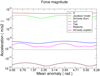Fig. 6 Acceleration magnitude over one orbit for each term.

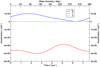Fig. 7 Difference between the Jacobson model (Eq. (19)) and the IT+CoT term of full mutual potential model.

4.1.4 Reference orbit

PDS (Planetary Data System) archives (Acton 1996; Acton et al. 2018) provide the up-to-date Phobos ephemeris in the file mar097.bsp. This was selected as the reference for comparison with all other orbits, since this reference is determined from observations that are astrometric in nature and that thus reflect precisely where Phobos is and how the body shape is oriented at all of the observation epochs. As is described in the orbit file documentation, it models Mars’ gravity, third body, and tides, although the implementation may differ from ours.

The main difference lies in the account of the Mars-Phobos mutual gravity: it is limited to a so-called libration term force and written as (Jacobson 2010) $$F_1=-\frac{3}{2}\mu \left(\frac{R^{\prime 2}}{r^4}\right)\left[\left(-C_{20}^{\prime }+6C_{22}^{\prime }\cos 2{\beta }^{\prime }\right)\stackrel{⌢}{r}+4C_{22}^{\prime }\sin 2{\beta }^{\prime }\stackrel{⌢}{t}\right],$$(19)

where µ is the GM of Mars, R′ the equatorial radius of Phobos, r the distance from Phobos to Mars, C′₂₀ the second degree zonal harmonic of Phobos, and C′₂₂ its second degree and order tesseral term. β′ equals $\alpha -{\text{Φ}}^{\prime },\widehat{r}$ is the unit vector directed from Mars toward Phobos, and $\widehat{t}$ is the unit vector in the Phobos orbit plane normal to $\widehat{r}$ and in the direction of Phobos’s orbital motion. This agrees with the degree two model presented in Appendix A, with some simplifications: it retains only one part of the indirect terms (IT) and none of the CoT due to assuming S′₂₂ = 0, and δ = 0.

4.2 Numerical results

4.2.1 Comparison of accelerations

Figure 6 shows the amplitudes of the total accelerations involved in the dynamics of Phobos over one revolution. The central and direct terms are the dominant ones but do not exhibit any particularity and are not shown; only accelerations between 10⁻⁶ and 10⁻¹² are presented.

The term “Jacobson model” represents the contribution of the mutual potential that Jacobson uses (Eq. (19)). This contribution is very close to the IT of our mutual potential model.

The CoT acceleration is of the same order as the effect of the Martian tide but larger. The contribution is therefore relatively small in the orbit of Phobos, though not negligible.

The smallest accelerations in Fig. 6 are the relativistic Schwarzschild effect and the contribution of the third body, Jupiter. Both are less than 10⁻¹⁰ m/s².

4.2.2 Jacobson model and full mutual potential impact

Figure 7 shows the difference in the RTN axis between the Jacobson acceleration, which assumes an equatorial and circular orbit and neglects terms of a degree greater than two, and the acceleration induced by the full mutual potential; that is, the complete IT and CoT terms.

In order to quantify the impact of the mutual potential, the numerically integrated trajectory of Phobos was compared with the Jacobson reference trajectory described in Sect. 4.1.4. The calculations were carried out over 3 days (72 hours). Firstly, the orbit generation and adjustment were made using the same dynamics as for the Jacobson trajectory. A second case was run with our full mutual potential model, followed by a similar adjustment on Jacobson orbit. The least-squares fit seeks to minimize the 3D residuals from the reference orbit, so in terms of orbital parameters we can observe a secular trend for certain parameters, which is due to the fit in the Cartesian domain over a relatively short period (3 days).

In the first case, a 3D RMS of less than 7 m over 3 days is obtained, which means the dynamical models are fairly consistent with the Jacobson ones. However, in the second case in which the full mutual potential is included, the 3D RMS rises to greater than 27 m.

Tables 6 and 7 respectively show the trajectory difference statistics in the RTN axes after the adjustment. As was expected, the impact of the difference in dynamical models is mainly on the tangential axis. The graphs in Fig. 8 show the evolution of the difference between the two adjusted trajectories, in terms of orbital parameters.

Figure 9 shows the differences in position (in R,T,N) between the Jacobson reference trajectory and our adjusted trajectories, without and with the full mutual potential modeling. On the butterfly shape inherent to the least squares adjustment, and on the once-per-revolution terms expected from the dynamics differences, was superimposed an along-track secular effect. This deviation from the Jacobson reference orbit was an order of magnitude smaller than the translation of the Phobos shape model in order to make the center of mass coincide with the shape’s center of figure (see Sect. 4.1.2). Therefore, it seems that the present uncertainty in Phobos’ internal mass distribution swamps the effects of including or not including the additional parts of the IT terms and the CoT terms that Jacobson did not include. Nevertheless, for future modeling of Phobos gravity field and mass distribution, we recommend including such terms, which otherwise would induce (additional) errors in any density model.

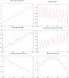Fig. 8 Difference between orbital parameters for case 1 and case 2. The X axis represents the number of Julian days since January 1, 1950 (day 27 709 = 12/11/2025).

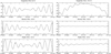Fig. 9 Position differences in tangential, normal, and radial between Jacobson Phobos orbit and our adjusted orbits: with a simplified model for the mutual potential (left) consistent with Table 6, and with a full mutual potential (right) consistent with Table 7 The X axis represents the number of Julian days since January 1, 1950 (day 27 709 = 12/11/2025).

5 Conclusion

We have shown that usually neglected terms in the expression of the mutual gravitational potential of two celestial bodies of an odd shape can have a significant dynamical effect on their relative orbit. In particular, the MMX mission at the Mars-Phobos system, to be launched in 2026, will bring a wealth of data, including new tracking measurements that will be used to improve our knowledge of Phobos and especially its ephemeris and gravity field model. Their determination process should take into account the indirect and coupling gravitational terms of the Mars–Phobos pair, as we do here.

Acknowledgements

Supports of CNES (Centre National d’Etudes Spatiales) and of OMP (Observatoire Midi-Pyrénées) are gratefully acknowledged. We thank the reviewers for very sharp remarks which greatly helped improving the paper.

Appendix A Case of degree and order-two coefficients in a simplified geometry

A special case is considered when the equatorial planes of the two bodies remain parallel to the [R⁰] reference system equator (Fig. A.1) and when the spherical harmonics are limited to degree and order two for each body. Direct formulas using un-normalized real spherical harmonic coefficients (C_lm, S_lm, C′_lm, S′_lm) can be derived and allow comparison with other authors’ results as well as numerical verification with the more general formulas applied to this case.

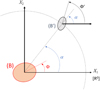Fig. A.1 Particular case (viewed from X3 > 0): Ψ= Ψ′ = Θ = Θ′ =0, and harmonic coefficients are limited to degree and order two for each body.

In this case, U becomes $$\tilde{U}=G\frac{M{M}^{\prime }}{r}\left(1+T_{20}+T_{02}+T_{22}\right).$$

The three terms are $$\begin{array}{l}{T}_{20}={\left(\frac{R}{r}\right)}^2\left[C_{20}{P}_{20}(\sin \delta )+\left\{C_{22}\cos 2\beta +S_{22}\sin 2\beta \right\}{P}_{22}(\sin \delta )\right]\\ T_{02}={\left(\frac{R^{\prime }}{r}\right)}^2[C_{20}^{\prime }{P}_{20}(\sin \delta )\\ +\left\{C_{22}^{\prime }\cos 2{\beta }^{\prime }+S_{22}^{\prime }\sin 2{\beta }^{\prime }\right\}{P}_{22}(\sin \delta )]\\ T_{22}={\left(\frac{R}{r}\right)}^2{\left(\frac{R^{\prime }}{r}\right)}^2\left[Q_{22}^0+Q_{22}^{\pm 2}\right],\end{array}$$

where $$\begin{array}{l}\begin{array}{l}{Q}_{22}^0=C_{20}\left[6C_{20}^{\prime }{P}_{40}(\sin \delta )+\left\{C_{22}^{\prime }\cos 2{\beta }^{\prime }+S_{22}^{\prime }\sin 2{\beta }^{\prime }\right\}{P}_{42}(\sin \delta )\right]\hfill \\ Q_{22}^{\pm 2}=\left[u_{22}\cos 2\left(\text{Φ}-{\text{Φ}}^{\prime }\right)+v_{22}\sin 2\left(\text{Φ}-{\text{Φ}}^{\prime }\right)\right]P_{40}(\sin \delta )\hfill \end{array}\\ \begin{array}{l}+C_{20}^{\prime }\left[C_{22}\cos 2\beta +S_{22}\sin 2\beta \right]P_{42}(\sin \delta )\hfill \\ +[w_{22}\cos \left[4\alpha -2\left(\text{Φ}+{\text{Φ}}^{\prime }\right)\right]\hfill \end{array}\\ +{ɀ}_{22}\sin \left[4\alpha -2\left(\text{Φ}+{\text{Φ}}^{\prime }\right)\right]]P_{44}(\sin \delta )\end{array}$$

and with β =α − Φ; β’ = α − Φ’ $$\begin{array}{c}{u}_{22}=12\left(C_{22}{C}_{22}^{\prime }+S_{22}{S}_{22}^{\prime }\right),v_{22}=12\left(C_{22}{S}_{22}^{\prime }-S_{22}{C}_{22}^{\prime }\right)\\ w_{22}=\left(C_{22}{C}_{22}^{\prime }-S_{22}{S}_{22}^{\prime }\right)/2,{ɀ}_{22}=\left(C_{22}{S}_{22}^{\prime }+S_{22}{C}_{22}^{\prime }\right)/2.\end{array}$$

As an example, note that Jacobson (2010) considered the term T₂₀ and only the portion of T₀₂ without S′₂₂ (with P₂₀(0) = −1/2, P_շշ(0) = 3)

Appendix B Phobos gravity model

The Phobos gravity field was calculated by transforming the body shape into gravity spherical harmonics, assuming a uniform mass distribution.

The algorithm involved calculating the gravity field modeled from the polyhedral shape on a sphere containing all the masses. The calculation was performed on a 0.1° grid in longitude and latitude using the “polyhedral-gravity-model” tool of Tsoulis (Tsoulis 2012; Tsoulis & Gavriilidou 2021). The projection on the spherical harmonics basis was then carried out using an internal tool.

The whole process was compared to another method (Balmino 1994) and gave consistent results. Table B.1 gives the normalized derived Phobos gravity field spherical harmonics. We have set the coefficients of degree 1 to 0.0 to align the center of the figure with the center of gravity, and the coefficients C₂₁ and S₂₁ to 0 also to align the main axis of inertia of the body with the Z axis of the frame of reference attached to the body.

References

All Tables

All Figures

	Fig. 1 Two bodies, (B) and (B′), and their body-fixed reference systems, [R] and [R′], respectively. [R0] and [R′0] are two other reference frames that have the same orientation in space.
In the text

	Fig. 2 Going from reference system [R0] to another one, [R], by means of the Euler angles, Ψ, Θ, and Φ.
In the text

	Fig. 3 Acceleration magnitudes of Dimorphos over one orbit for the direct term (DT).
In the text

	Fig. 4 Acceleration magnitudes of Dimorphos over one orbit for IT.
In the text

	Fig. 5 Acceleration magnitudes of Dimorphos over one orbit for CoT.
In the text

	Fig. 6 Acceleration magnitude over one orbit for each term.
In the text

	Fig. 7 Difference between the Jacobson model (Eq. (19)) and the IT+CoT term of full mutual potential model.
In the text

	Fig. 8 Difference between orbital parameters for case 1 and case 2. The X axis represents the number of Julian days since January 1, 1950 (day 27 709 = 12/11/2025).
In the text

	Fig. 9 Position differences in tangential, normal, and radial between Jacobson Phobos orbit and our adjusted orbits: with a simplified model for the mutual potential (left) consistent with Table 6, and with a full mutual potential (right) consistent with Table 7 The X axis represents the number of Julian days since January 1, 1950 (day 27 709 = 12/11/2025).
In the text

	Fig. A.1 Particular case (viewed from X3 > 0): Ψ= Ψ′ = Θ = Θ′ =0, and harmonic coefficients are limited to degree and order two for each body.
In the text

References

- Acton, C. H. 1996, Planet. Space Sci., 44, 65 [Google Scholar]
- Acton, C., Bachman, N., Semenov, B., & Wright, E. 2018, Planet. Space Sci., 150, 9 [Google Scholar]
- Archinal, B. A., Acton, C. H., A’Hearn, M. F., et al. 2018, Celest. Mech. Dyn. Astron., 130, 22 [Google Scholar]
- Archinal, B. A., Acton, C. H., Conrad, A., et al. 2019, Celest. Mech. Dyn. Astron., 131, 61 [Google Scholar]
- Balmino, G. 1994, Celest. Mech. Dyn. Astron., 60, 331 [NASA ADS] [CrossRef] [Google Scholar]
- Balmino, G., & Borderies, N. 1978, Celest. Mech., 17, 113 [NASA ADS] [CrossRef] [Google Scholar]
- Balmino, G., Barriot, J. P., & Valès, N. 1990, Manuscr. Geod., 15, 11 [NASA ADS] [CrossRef] [Google Scholar]
- Borderies, N. 1978, Celest. Mech., 18, 295 [NASA ADS] [CrossRef] [Google Scholar]
- Borderies, N., & Yoder, C. F. 1990, A&A, 233, 235 [NASA ADS] [Google Scholar]
- Boyce, W. 1997, Celest. Mech. Dyn. Astron., 67, 107 [NASA ADS] [CrossRef] [Google Scholar]
- Daly, R. T., Ernst, C. M., Barnouin, O. S., et al. 2023, Nature, 616, 443 [CrossRef] [Google Scholar]
- Ernst, C. M., Daly, R. T., Gaskell, R. W., et al. 2023, Earth Planets Space, 75, 103 [NASA ADS] [CrossRef] [Google Scholar]
- ESA 2022, https://www.heramission.space [Google Scholar]
- Folkner, W. M., Williams, J. G., Boggs, D. H., Park, R. S., & Kuchynka, P. 2014, Interplanetary Network Progress Report, 42-196, 1 [Google Scholar]
- Huang, C., & Liu, L. 1992, Celest. Mech. Dyn. Astron., 53, 293 [NASA ADS] [CrossRef] [Google Scholar]
- Jacobson, R. A. 2010, AJ, 139, 668 [Google Scholar]
- Jacobson, R. A., & Lainey, V. 2014, Planet. Space Sci., 102, 35 [CrossRef] [Google Scholar]
- Konopliv, A. S., Park, R. S., & Folkner, W. M. 2016, Icarus, 274, 253 [Google Scholar]
- Kuramoto, K., Kawakatsu, Y., Fujimoto, M., et al. 2022, Earth Planets Space, 74, 12 [NASA ADS] [CrossRef] [Google Scholar]
- Park, R. S., Folkner, W. M., Williams, J. G., & Boggs, D. H. 2021, AJ, 161, 105 [NASA ADS] [CrossRef] [Google Scholar]
- Space Geodesy, C. s. 2018, Algorithmic documentation of the GINS software, Tech. rep., CNES [Google Scholar]
- Tsoulis, D. 2012, Geophysics, 77, F1 [NASA ADS] [CrossRef] [Google Scholar]
- Tsoulis, D., & Gavriilidou, G. 2021, Geophys. Prospect., 69, 1745 [NASA ADS] [CrossRef] [Google Scholar]
- Wigner, E. P., & Fano, U. 1960, Am. J. Phys., 28, 408 [NASA ADS] [CrossRef] [Google Scholar]
- Yang, Y., Yan, J., Jian, N., Matsumoto, K., & Barriot, J.-P. 2024, A&A, 685, A13 [NASA ADS] [CrossRef] [EDP Sciences] [Google Scholar]
All Tables
Adjustment on the Jacobson orbit of the Phobos trajectory without full mutual potential.
Adjustment on the Jacobson orbit of the Phobos trajectory with full mutual potential.