| Issue |
A&A
Volume 694, February 2025
|
|
|---|---|---|
| Article Number | A19 | |
| Number of page(s) | 12 | |
| Section | Galactic structure, stellar clusters and populations | |
| DOI | https://doi.org/10.1051/0004-6361/202452698 | |
| Published online | 31 January 2025 | |
Yields from massive stars in binaries
Chemical evolution of the Milky Way disk
1
Dipartimento di Fisica, Sezione di Astronomia, Università di Trieste,
Via G.B. Tiepolo 11,
34143
Trieste,
Italy
2
Dipartimento di Fisica e Astronomia “Augusto Righi”, Alma Mater Studiorum, Università di Bologna,
Via Gobetti 93/2,
40129
Bologna,
Italy
3
INAF – Osservatorio di Astrofisica e Scienza dello Spazio di Bologna,
Via Gobetti 93/3,
40129
Bologna,
Italy
4
INAF – Osservatorio Astronomico di Trieste,
via G.B. Tiepolo 11,
34131,
Trieste,
Italy
5
INFN – Sezione di Trieste,
via Valerio 2,
34134
Trieste,
Italy
6
IFPU Institute for Fundamental Physics of the Universe,
Via Beirut 2,
34151
Trieste,
Italy
★ Corresponding authors; This email address is being protected from spambots. You need JavaScript enabled to view it.
; This email address is being protected from spambots. You need JavaScript enabled to view it.
; This email address is being protected from spambots. You need JavaScript enabled to view it.
Received:
22
October
2024
Accepted:
6
December
2024
Abstract
A large fraction of massive stars in the Galaxy reside in binary systems and their evolution is different from that of single stars. The yields of massive stars, which produce the majority of the metals in the Universe, could therefore be affected by the binary nature of the systems. However, very few studies have explored the effects of massive interacting binaries on the chemical evolution of the Milky Way. Recently, new grids of yields have been computed for single and binary-stripped massive stars with solar chemical composition. The main purpose of the present study is to test whether the results from these yields agree with models of the chemical evolution of Galactic stars. To this end, we adopted well-tested chemical evolution models for the Milky Way disk, implementing these yields for both single and binary-stripped massive stars. In particular, we assume different percentages of massive binary systems within the initial mass function. We computed the evolution of 22 chemical species starting from 4He to 64Zn, including CNO, α-elements, and Fe-peak elements. Our main results can be summarized as follows: (i) When adopting the new computed yields, large differences are found relative to the solar abundances predicted by chemical evolution models that adopt “standard” massive star yields from the literature for 12C, 14N, 24Mg, 39K, 40Ca, 55Mn, and 59Co. Generally, the yields for single stars reproduce the observed solar abundances slightly better, although for several elements a large fraction of binaries helps to reproduce the observations. (ii) Using different fractions of massive binaries (from 50% to 100%) leads to negligible differences in the predicted solar abundances, whereas these differences are more marked between models with and without binary-stripped stellar yields. (iii) Regarding [X/Fe] versus [Fe/H] relations, the yields including massive stars in binaries produce the best agreement with observational data for 52Cr, while for 12C, 39K, 40Ca, and 24Mg the best agreement with observational data are obtained with Farmer’s yields with no binaries.
Key words: ISM: abundances / Galaxy: abundances / Galaxy: disk / Galaxy: evolution / Galaxy: formation
© The Authors 2025
 Open Access article, published by EDP Sciences, under the terms of the Creative Commons Attribution License (https://creativecommons.org/licenses/by/4.0), which permits unrestricted use, distribution, and reproduction in any medium, provided the original work is properly cited.
This article is published in open access under the Subscribe to Open model. This email address is being protected from spambots. You need JavaScript enabled to view it. to support open access publication.
1 Introduction
Galactic archaeology is the study and interpretation of the observed chemical abundances in stars and gas in order to reconstruct the history of the star formation and evolution of our Galaxy and external ones. Among the different processes that need to be taken into account when computing the chemical evolution of galaxies, stellar yields – the amounts of the different chemical elements produced by stars and ejected into the interstellar medium (ISM) – are a key ingredient required to properly model the chemical enrichment in galaxies, but are also the most important source of intrinsic uncertainty within models (see, e.g., Romano et al. 2010; Matteucci 2021, and references therein).
Detailed models of galactic chemical evolution include the yields of a large network of chemical elements, from hydrogen up to the heaviest elements, such as 63Cu and 64Zn. Most of the metal mass is formed in massive stars (M ≳ 10 M⊙), which end their lives as core-collapse supernovae (CC-SNe). Generally, in models of galactic chemical evolution, only the yields from single massive stars are considered (e.g., Woosley & Weaver 1995; Kobayashi et al. 2006; Nomoto et al. 2013; Limongi & Chieffi 2018, but see De Donder & Vanbeveren 2004), as large grids of stellar masses and elemental abundance yields are only available for single stellar models. However, stars preferentially form in clusters and associations (Lada & Lada 2003), where interactions are frequent. Indeed, binary stars are common, and binarity has been shown to influence stellar evolutionary paths and the nucleosynthesis products relative to the case of single stars (see, e.g., Langer 2012; Woosley 2019). During the evolution of a binary system, several common-envelope phases can occur, including episodes of mass transfer and stripping in stars, and these influence the production of elements, as the matter accreted, or stripped, is made available to, or is removed from, subsequent nuclear processing.
To date, the only study focusing on the effect of binaries on the chemical evolution of the Milky Way (MW) is that of De Donder & Vanbeveren (2002). These authors computed chemical yields from massive stars in binaries and tested them in a two- infall chemical model for the MW similar to that of Chiappini et al. (1997). Their results showed that including massive binaries improves the agreement with the time evolution of carbon abundance and suggested that binary evolution can drive the production of primary nitrogen from massive stars; although nitrogen is also provided by single rotating massive stars (e.g., Meynet & Maeder 2002; Limongi & Chieffi 2018). On the other hand, De Donder & Vanbeveren (2002) concluded that accounting for the chemical enrichment driven by massive binaries produces a variation in the evolution of other chemical elements (He, O, Ne, Mg, Si, S, and Ca) of no more than a factor of 2 relative to the evolution without binaries.
Recently, Farmer et al. (2023) published yields for massive stars in binary systems for a greater number of chemical species than those included in the computations of De Donder & Vanbeveren (2002) and showed that differences in the production of elements in the presence of binaries only exist for specific elements. For example, Farmer et al. (2023) showed that in these binary-stripped stars there is an increased production of F and K relative to single stars.
In the present paper, we adopt a detailed and well-tested (e.g., Spitoni et al. 2019; 2020; Palla et al. 2020; Palla 2021) chemical evolution model for the MW, which allows us to follow the evolution of the abundances of several species (H, He, C, N, α- elements, Fe, and Fe-peak elements). In particular, for the first time, we introduce the yields of Farmer et al. (2023) for single and binary-stripped stars into chemical evolution models for the MW and predict the solar chemical abundances as well as the [X/Fe] versus [Fe/H]1 relations, where X are all the elements except Fe (the most commonly used tracer of stellar metallicity). The results of the models are then compared with abundance patterns derived from the observations of large-scale surveys (APOGEE; Abdurro’uf et al. 2022) as well as smaller programs at higher spectral resolution (e.g., Bensby et al. 2014; Nissen et al. 2020) to test whether the yields adopted in this work can improve the agreement between the predicted abundance trends and observations in the MW disk.
The paper is organized as follows: in Sect. 2 we describe the chemical evolution model, with a special focus on the description of the adopted stellar yields both for single and binary massive stars. In Sect. 3, we describe the observational data adopted for comparison with our results. In Sect. 4, we show and discuss the results of our predictions compared to observations, and in Sect. 5 we outline our conclusions.
2 Chemical evolution framework
In this section, we present the chemical evolution models adopted throughout our work. The models used are as follows:
The one-infall model (as proposed by Chiosi 1980; Matteucci & Greggio 1986; Matteucci & Francois 1989; Boissier & Prantzos 1999), as described in Matteucci (2021), which assumes that the Galactic disk components form sequentially as a result of a single infall episode of primordial gas, with a timescale of τ ≃ 7 Gyr for the solar vicinity, in order to reproduce the G-dwarf metallicity distribution (Matteucci 2012).
A revised two-infall model (e.g., Palla et al. 2020), which assumes that the MW disk forms in two separate and sequential gas-accretion episodes. The first episode forms the chemical thick disk2 on a timescale of τ1 ≃ 1 Gyr, while the second forms the chemical thin disk on a longer timescale of τ2 ≃ 7 Gyr. The term “revised” refers to the adoption of a larger delay of 3.25 Gyr between the first and second infall episodes, as opposed to the “classical” delay of 1 Gyr (Chiappini et al. 1997; Romano et al. 2010). The adopted assumptions in the “revised” two-infall model allow us to reproduce large-survey abundance data (Palla et al. 2020; Spitoni et al. 2021), as well as abundance–age diagrams (Spitoni et al. 2019; Spitoni et al. 2020) in the solar neighborhood.
2.1 Chemical evolution models
In both the models described above, the basic equation used to describe the evolution of an element i in the ISM is (see Matteucci 2021):
 (1)
(1)
On the left-hand side, σi(R, t) = σɡas(R, t)Xi(R, t) is the fractional surface mass density of the element i in the ISM at the time t, with Xi(R, t) being the mass abundance of that element and σɡas(R, t) the mass density of the ISM. The first term on the right-hand side represents the rate at which chemical elements are subtracted from the ISM by star formation, with ψ(R, t) being the star-formation rate (SFR), parameterized according to the Schmidt-Kennicutt law (Kennicutt 1998):
 (2)
(2)
where k = 1.5, and ν is the star formation efficiency expressed in units of Gyr−1 and considered to be variable with Galactocentric distance, as in Palla et al. (2020).
The second term of the equation, Ṙi(R, t), refers to the mass returned to the ISM in form of the new and old chemical element i. It represents the rate at which chemical elements are returned to the ISM through stellar winds and supernova explosions. The term Ri(R, t) also depends on the initial mass function (IMF), here parameterized as in Kroupa et al. (1993).
The last term in the equation,  , is the gas-infall rate, which in the one-infall model is computed as:
 (3)
(3)
where τ is the infall timescale, Xi,inf is the composition of the infalling gas (assumed to be primordial), and A(R) is the normalizing factor that is chosen to reproduce the total surface mass density observed at present at each radius (see also Palla 2021).
For the two-infall scenario, the gas-infall rate is instead computed as
 (4)
(4)
where τ1 and τ2 are the infall timescales for first and second infall episode, respectively, tmax is the time of maximum infall, which is also the delay between the two episodes, and A(R) and B(R) are the coefficients obtained by reproducing the present-day surface mass density of the thick and thin disks in solar neighborhood. We also remind the reader that θ in the equation above is the Heaviside step function.
In addition to the CC-SN rate, the model includes a detailed computation of the Type Ia supernova (SN Ia) rate assuming the single degenerate scenario and in particular the delay-time- distribution (DTD) function as computed by Matteucci & Recchi (2001), which can be considered a good compromise to describe the delayed pollution from the entire SN Ia population (see Palla 2021 and references therein). We note that neither of the above models assumes the presence of galactic winds. Melioli et al. (2008, 2009) and Spitoni et al. (2008, 2009), while investigating Galactic fountains caused by Type II supernova (SNe II) explosions in OB associations within the solar annulus, found that the metals ejected by these events fall back to nearly the same Galactocentric region from which they originated, and thus have little effect on the overall chemical evolution of the Galactic disk. Moreover, these findings were recently confirmed by Hopkins et al. (2023), who showed that the vast majority of the mass ejected from the disk is accreted again on short timescales and near to the original ejection site (Galactic fountains).
2.2 Nucleosynthesis prescriptions
In this work, we adopt for the first time the stellar yields of Farmer et al. (2023) for massive stars in the context of well-tested models of chemical evolution for the MW. Farmer et al. (2023) estimate stellar yields for elements up to Zn for an extensive grid (Mini = 11–45 M⊙) of both single and binary-stripped stars at solar metallicity using the MESA stellar evolution code (version 12115, see e.g. Paxton et al. 2011, 2013; 2015; 2018; 2019; Jermyn et al. 2023). In Farmer et al. (2023), stars are evolved from the zero-age main sequence (ZAMS) to core-collapse and then supernova until shock breakout. The assumed stellar chemical composition in the models is the solar one (Grevesse & Sauval 1998). For binary stars, Farmer et al. (2023) evolve the primary star considering a companion with a mass ratio of M2/M1 = 0.8 and an initial orbital period of between 38 and 300 days in order to assure that all the binary stars undergo case B3 mass transfer (Paczyński 1967; van den Heuvel 1969). For these systems, the secondary star is modeled as a point mass until the end of core- helium burning, at which point the secondary is removed and the primary star evolves until core collapse (see Laplace et al. 2020). Therefore, the resulting yields refer only to the primary star in the binary system. In both single and binary cases, stellar models are non-rotating. For more details about the choice of physics and model assumptions, we refer to Farmer et al. (2021, 2023) and Laplace et al. (2020, 2021).
In this study, we adopt different fractions of massive star binaries in the IMF to explore the effect of binary-stripped stars on chemical enrichment. More specifically, we test the cases of 100%, 70%, 50%, and 0% massive star binaries. The reason for passing from a binary fraction of 0% to 50% is that, if we assume binary percentages of lower than 50%, we see negligible differences in the results relative to the case with no binaries.
To make a comparison between the newly proposed yields by Farmer et al. (2023) and other well-tested yields for single massive stars from the literature, we also adopt the yield sets suggested in Romano et al. (2010, their model 15). In particular, these yields consist in a combination of models obtained with the Geneva stellar evolutionary code (Meynet & Maeder 2002; Hirschi 2005, 2007; Ekström et al. 2008) for elements lighter than O, and those of Kobayashi et al. (2006) for heavier elements (see Romano et al. 2010 for more details).
Despite focusing on the outcome of different massive star yields, the model also includes the nucleosynthesis from low- and intermediate-mass stars (LIMS) and SNe Ia to properly account for the Galaxy chemical evolution. In order to highlight the different enrichment from different massive star yields, we adopt the yields of Karakas (2010) for LIMS and those of Iwamoto et al. (1999, their W7 model) for SNe Ia for all the models of this paper.
3 The data sample
In this study, we use the abundances of solar neighborhood stars as measured in APOGEE DR17 (Abdurro’uf et al. 2022), Bensby et al. (2014), and Nissen et al. (2020). In the following, we provide further details of the different datasets adopted, also specifying which chemical elements are selected to perform our comparison.
3.1 The APOGEE DR17 data sample
Throughout this work, we adopt data from the high-resolution spectroscopic survey APOGEE DR17 (Abdurro’uf et al. 2022), which is part of the Sloan Digital Sky Surveys (SDSS). APOGEE operates using the du Pont Telescope and the Sloan Foundation 2.5 m Telescope (Gunn et al. 2006) at Apache Point Observatory. Stellar parameters and abundances are derived using the APOGEE Stellar Parameters and Chemical Abundance Pipeline (ASPCAP; García Pérez et al. 2016). The model atmospheres used in APOGEE DR17 are based on the MARCS model (Gustafsson et al. 2008), as discussed by Jönsson et al. (2020), and the line list is described in Smith et al. (2021).
Here, we consider only stars with a Galactocentric distance of 7 kpc ≤ RGC ≤ 9 kpc as computed in Leung & Bovy (2019) and reported in the value-added astroNN4 catalog, where accurate distances for distant stars are obtained using a deep neural network trained on parallax measurements of nearby stars shared between Gaia (Gaia Collaboration 2016, 2021) and APOGEE. Following the work of Spitoni et al. (2024), we also applied a further selection based on signal-to-noise ratio (S/N) and vertical height above and below the Galactic plane (|z|): S/N>80 and |z|≤2 kpc. This selection leaves us with a sample of around 55 111 total stars, with 55 016 spectra observed for C, 55 042 for O, 55 047 for Mg, 54 765 for K, 55 015 for Ca, 53 445 for Ti, and 53 267 for Cr.
3.2 Bensby et al. (2014) and Nissen et al. (2020) datasets
In addition to the APOGEE data, in this work we consider abundance data from small programs also targeting disk stars (Bensby et al. 2014; Nissen et al. 2020), but in the optical wavelength range at very high spectral resolution (R/RAPOGEE > 2). In this way, we can make a further comparison with the predicted trends, as we are probing a very different observational setup that may lead to differences in the derived abundances (e.g., Spina et al. 2022; Hegedűs et al. 2023, see also later in the text).
In Bensby et al. (2014), chemical abundances were derived for 714 FG dwarf and subgiant stars in the solar neighborhood. Observations were conducted using various spectrographs (e.g., FIES, UVES, HARPS, and MIKE) at multiple observational facilities (e.g., NOT, VLT, La Silla 3.6 m, Magellan Clay). All observations were carried out at a resolution of R > 40 000, achieving high S/Ns (>150). In this study, we adopt the stellar abundances of Fe, O, Mg, Ca, Ti, and Cr measured for all 714 stars in the original Bensby et al. (2014) sample.
The abundances from Nissen et al. (2020), on the other hand, were derived from very high-resolution (R > 100000), high-S/N (>600) observations of 72 solar twin stars obtained using the HARPS and HARPS-N spectrographs at the La Silla 3.6 m and TNG telescopes. These data provide highly precise measurements of elemental abundances in the solar vicinity. For this study, we adopt the stellar abundances of Fe, C, O, Mg, Ca, Ti, and Cr for all stars in the Nissen et al. (2020) sample.
Models adopted in this work.
4 Results
In this section, we show the results obtained by our chemical evolution models testing different setups for CC-SN yields, including models of stars in binary systems. We have chosen to show two different kinds of models, one-infall and two- infall, because although the one-infall model is only good for describing the evolution of the thin disk, it reveals the predicted behaviors of the [X/Fe] versus [Fe/H] relations more clearly, and allows an easier comparison between cases with different stellar yields. On the other hand, the two-infall model provides a more realistic description of the evolution of the thick and thin disk.
The models and their prescriptions are reported in Table 1, where we show the model name in the first column, the adopted massive star yields in the second column, the percentage of binaries considered in the case of adoption of the Farmer et al. (2023) yields in the third column, and whether we adopt a one-infall or two-infall scheme for chemical evolution. In the remainder of the paper, we refer to the models labeled with “K0” as Reference Models, as they adopt well-tested yield sets from the literature for single massive stars, as described in Sect. 2.2 (see Romano et al. 2010). All the other models refer to the yields of Farmer et al. (2023) for massive stars, while the yields for other stellar types are the same as in K0 models (see Sect. 2.2). The numbers 1 and 2 in the labels of the models refer to the one- and two-infall models, respectively. It is worth noting that the K0 Reference Models take into account exactly the same physical assumptions as the other models, as described in Sect. 2, except for the yields from massive stars, which are those adopted in Romano et al. (2010), as described in Sect. 2.2.
4.1 Solar abundances
In this first part, we show the model predictions obtained for the solar abundances, namely the ISM abundances at the time of the birth of our Sun. Model abundances are taken at an age of 4.5 Gyr ago, which is the time at which the proto-solar cloud was formed, and are compared with measured solar abundances as obtained by Asplund et al. (2009).
Table 2 shows the solar abundances as predicted by the two- infall model, and more specifically the abundances by number (12 + log(X/H)) of 22 elements from He to Zn. As explained in Sect. 2, the adopted chemical evolution model has already been tested in several studies and allows us to best reproduce the multiple constraints coming from abundance patterns and ages in the solar vicinity (e.g., Spitoni et al. 2019, 2020; Palla et al. 2020, Molero et al. 2023). Therefore, the model outputs can be used for an insightful comparison with the measured solar abundances. Column 1 of Table 2 lists the chemical species, Column 2 the observed solar abundances, and Column 3, 4, 5, and 6 list the predictions from the models.
From the table, we see that once Farmer et al. (2023) stellar yields are used, different percentages of binary stars result in negligible variations for most of the chemical elements. The only notable differences are observed for 39K, 48Ti , and 51V. On the other hand, more marked variations are seen between the results obtained with the yields of Farmer et al. (2023) and those obtained with the yields of Romano et al. (2010, i.e., our Reference Model, K0-2). In particular, the Reference Model better reproduces the solar abundances of 19F, 23Na, 27Al, 28Si, 32S, 51V, 63Cu, and 64Zn, whereas 12C, 24Mg, 39K, and 40Ca solar abundances are much better reproduced by models using the Farmer et al. (2023) stellar yields. On the other hand, for 39K, the yields of Farmer et al. (2023) only well reproduce the solar abundance in the case where no binaries are assumed (Model F0- 2). However, it should be noted that, while the yields of Romano et al. (2010) are metallicity dependent, those of Farmer et al. (2023) are computed only for the solar chemical composition, thus making such a comparison more difficult (see Sect. 4.3).
These differences are even more evident when we observe Fig. 1, where we show the difference between the model predictions and the data from Asplund et al. (2009) for each element, as reported in Table 2. The chemical elements in this figure are identified by the atomic mass number (A) of their main isotopes.
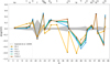 |
Fig. 1 ∆log(X/H) ratios for different elements as predicted by the two-infall model for different stellar yields and percentage of binaries (see legend). The tin gray dashed line indicates the solar ratios as measured in Asplund et al. (2009), while the gray shaded region is the abundance uncertainty. |
4.2 Chemical abundance patterns
In this section, we present the results of [X/Fe] versus [Fe/H] abundance ratios for our adopted models, testing different stellar yield prescriptions. It is worth noting that, during this section, we display the results for both the one-infall and the two- infall scenarios. More specifically, we use the one-infall scenario to compare the models in terms of their abundance evolution predictions, while the two-infall scenario is used to compare the chemical evolution models with the data as described in Sect. 3. This choice is justified by the fact that the outputs of the one-infall scenario allow us to highlight and better explain the effects produced by the different yields for massive stars on the predicted abundance patterns, whereas the more physically robust star formation history of the two-infall model is better suited to reproducing the observed abundance trends in the solar neighborhood.
In the following, we show the model results for the chemical elements that are most relevant to our study. In particular, we focus on the chemical abundances for which we have a large amount of data and we observe important differences in the evolution of the [X/Fe] versus [Fe/H] abundance patterns for different yield prescriptions. In the [X/Fe] plots, we always use the same color system for the same four models, as already used in Fig. 1. Moreover, as Farmer et al. (2023) yields are only computed for the solar metallicity, we also excluded from the analysis those elements that are known to show a marked dependence on metallicity, namely the elements with a prominent secondary5 component (see Sect. 4.3).
4.2.1 α-elements
We start our analysis from 12C and the most relevant α-elements, namely 16O, 24Mg, 40Ca, and 48Ti. It is worth noting that all the model outputs and stellar data are normalized to Asplund et al. (2009) solar abundances, in agreement with the data presented in Sect. 3.
It is also worth noting that the following [X/Fe] versus [Fe/H] diagrams have to be interpreted according to the time-delay model (Tinsley 1980; Greggio & Renzini 1983; Matteucci & Greggio 1986; Matteucci 2012, 2021). The time-delay interpretation is grounded in the fact that the [Fe/H]-axis can be interpreted as a time evolution axis. Therefore, at low metallicities (hence at earlier times), there is a predominant contribution to metals from massive stars and only at larger metallicities is there a substantial production of Fe from Type Ia SNe, which start exploding with a delay relative to CC-SNe and can have explosion times of as long as the Hubble time. According to this, the [α/Fe] ratios show the so-called plateau at low metallicities ([Fe/H] ≲ −1.0 dex in the MW), and then decline for larger metallicities as α-elements are presumed to be predominantly produced by CC-SNe. If the element considered is instead produced in greater amounts by Type Ia SNe and/or by low- and intermediate-mass stars, the change in slope at intermediate to high metallicity is less marked and becomes null or even positive when the element is produced mostly by delayed sources.
We note that the behaviors of the above elements relative to Fe are different for the one-infall and two-infall models. In the latter, which is best suited to reproducing the multiple features observed in the MW disk, there is a natural gap in the SFR between the formation of the chemical thick and thin disks. This gap produces the loops observed in the bottom panels of the following figures. This behavior is the consequence of a delayed second gas infall, which dilutes the ISM with primordial gas, lowering the [Fe/H] ratio and leaving the [X/Fe] unchanged. The metal abundance is then restored thanks to the subsequent episode of star formation (see also Spitoni et al. 2019).
For a more detailed analysis of the chemical abundance evolution, in Fig. 2, we compare results from our models for [C/Fe] versus [Fe/H]. In the upper panel, we compare the one-infall model (with the Reference Model being K0-1) for different percentages of binaries, namely 0%, 70%, and 100%, in the IMF of massive stars. Models that use Farmer et al. (2023) yields show an almost typical α behavior, with a plateau or slow decrease in the [C/Fe] ratio at low metallicity, a knee around [Fe/H] ~−1 dex, and a steeper decrease at high metallicity. Moreover, we observe that models with higher binary fractions tend to rise the level of the plateau, highlighting that yields from binary massive stars predict a larger C enrichment (see Farmer et al. 2021, Romano 2022). The same α-element behavior is instead not observed in the Reference Model, which has the same yield prescription as model 15 in Romano et al. (2010): for this model, we observe a steep decrease in [C/Fe] at low metallicity followed by an increase (at [Fe/H] ≃−1 dex) and again a decrease in this ratio. The lower [C/Fe] ratios predicted by the Reference Model are due to the lower C yields (Meynet & Maeder 2002; Hirschi 2007; Ekström et al. 2008) at low metallicities, with only a significant contribution from extremely metal-poor massive stellar rotators (EMP, [Fe/H] <−3 dex). Due to the lower ratio at metallicities around [Fe/H] ~−1 dex, the Reference Model shows a prominent bump due to the contribution of low-mass AGB stars to the carbon enrichment (see also Romano et al. 2019; Ventura et al. 2022), which is instead almost hidden in the models adopting Farmer et al. (2023) yields. However, the comparison shows that the larger C yields in metal-rich SNe in the Reference Model prevent the steep decrease in [C/Fe] and produce an excessively large ratio at solar metallicity, at variance with what happens using Farmer et al. (2023) yields.
In the lower panel of Fig. 2, we compare results from the K0-2 (Reference Model), F0-2, F70-2, and F100-2 models for [C/Fe] versus [Fe/H] with data from stars in the solar vicinity, as described in Sect. 3. All the models displayed in the lower panel show some difficulty in reproducing the trends shown by the data. In particular, the Reference Model K0-2 severely overestimates the data from Nissen et al. (2020) and APOGEE (Abdurro’uf et al. 2022) at [Fe/H] >−0.5 dex, while it aligns with the trend observed at lower metallicities (see also Romano et al. 2010; Romano et al. 2019). On the other hand, the models using Farmer et al. (2023) yields overestimate the observed [C/Fe] ratio at low metallicities; although they are in relatively good agreement with the sample of Nissen et al. (2020) and APOGEE (Abdurro’uf et al. 2022) data at solar and super-solar metallici-ties. Therefore, the massive star yields of Farmer et al. (2023) are better tracers of the C enrichment at high metallicities, whereas those of Kobayashi et al. (2006) are in better line with the trends observed at lower metallicities.
In Fig. 3, we compare results from our models for [O/Fe] versus [Fe/H]. The upper and lower panels show the results of the same models as in Fig. 2, and all the subsequent figures follow the same scheme. All the models presented in the upper panel of Fig. 3 show the characteristic α-element behavior, with a plateau or shallow slope at low metallicity and a steeper slope at higher metallicity, with a knee around [Fe/H] ~−1 dex. This is the typical behavior of the “time-delay model” (see Tinsley 1980; Greggio & Renzini 1983; Matteucci & Greggio 1986; Chiappini et al. 1997; Matteucci 2012, 2021). The models adopting Farmer et al. (2023) yields follow the same trend. However, it is worth noting that models assuming higher binary fractions show a lower [O/Fe] ratio, at variance with what is seen for C. This is due to the fact that a higher production of C from massive stars necessarily results in a decrease in O production, because the larger amount of C produced and ejected through stellar winds (see Farmer et al. 2021,2023) is no longer further processed into O. For what concerns the Reference Model, the predicted [O/Fe] ratios have similar values to those in the models adopting Farmer et al. (2023) yields at low metallicities, and slightly lower values for [Fe/H] >−2.25 dex, evidencing the lower O yields, especially for massive stars with m < 20 M⊙.
In any case, all the models shown in the upper panel of Fig. 3 show super-solar [O/Fe] values at all metallicities. This is reflected in the comparison with the solar vicinity data in the lower panel, where the models generally overestimate the observed [O/Fe] trends in different stellar samples. In particular, the Model F0-2 (using Farmer et al. 2023 yields assuming single stars only) does not match any of the survey data, while the other models (in particular the Reference Model K0-2) better reproduce the observed trends at low metallicity and especially the data by Bensby et al. (2014). Nonetheless, the overestimation of the [O/Fe] ratio by the different chemical evolutionary tracks around the solar metallicity remains evident, thus suggesting a significantly lower O ejection by massive stars relative to what is predicted by the different stellar models.
Figure 4 shows results for Mg. The Reference Model adopting Kobayashi et al. (2006) yields shows the typical α-element trend, with a plateau at low metallicity and a steep decrease in the [Mg/Fe] ratio after [Fe/H] ~−1 dex. All models using yields from Farmer et al. (2023) show a similar pattern, typical of α-elements. However, Farmer et al. (2023) models generally predict a higher value of the [Mg/Fe] ratio at all metallicities, especially when only single-star yields are employed, relative to the predictions by the Reference Model K0-2. It is worth noting that the differences in the yields of Mg for single massive stars of Farmer et al. (2023) and those of Kobayashi et al. (2006) are mainly due to the assumption of overshooting during C burning in Farmer et al. (2023) models, which is missing from the models by Kobayashi et al. (2006) (see also Tominaga et al. 2007). This assumption may not only have a significant impact on the C yields, as the 12C yield is sensitive to the size of the pocket of C that survives, which will then also affect the products of carbon burning, namely 20Ne, 23Na, and 24Mg, and successive burnings leading to heavier elements (see, e.g., Farmer et al. 2021, 2023).
Returning to the difference observed in the chemical patterns in the upper panel of Fig. 4, this difference is also evident in the lower panel of Fig. 4: more specifically, the Reference Model shows a lack of agreement with the observational data from APOGEE (Abdurro’uf et al. 2022), Bensby et al. (2014), and Nissen et al. (2020), with a clear underestimation of the observed trend especially at high metallicities (see also Palla et al. 2022 for a comparison with a different sample of survey data). On the other hand, the two-infall models adopting different Farmer et al. (2023) yield sets show better agreement with all the data adopted in this study. Focusing in particular on the APOGEE (Abdurro’uf et al. 2022) survey, we note that the F0-2 Model (assuming no binary-stripped star models) shows remarkable agreement with both the observed high-α and low-α sequences. This agreement is slightly poorer when we increase the binary fraction in the models. However, the chemical tracks are still consistent with observations from the different data samples.
Another α-element that shows quite significant variations in response to the different studied yield sets is Ca. In Fig. 5, we compare results from our models for [Ca/Fe] versus [Fe/H]. The upper panel highlights a different behavior both between Kobayashi et al. (2006) and Farmer et al. (2023) yield sets and between binary-stripped and single star models from Farmer et al. (2023). The model implementing Kobayashi et al. (2006) shows a lower [Ca/Fe] enrichment before and after the knee caused by the Type Ia SNe Fe production, with subsolar [Ca/Fe] values at high metallicities and an offset of the order of ~0.15 dex relative to Farmer et al. (2023) yield sets. For different Farmer et al. (2023) models, instead we see that while single-star yields produce a very flat plateau already at [Fe/H] ≲ −3 dex, models with increasing binary fractions show lower values at such low metallicities. This implies a significantly lower contribution to Ca enrichment from high-mass (m ≳ 20 M⊙; i.e., the first enriching with metals the ISM) binary-stripped stars, and a higher contribution from binary-stripped massive stars with lower masses (m ≲ 20 M⊙).
In the lower panel of Fig. 5, we see that the Reference Model does not agree with the observational data, as it clearly underproduces [Ca/Fe] at all metallicities (see also Romano et al. 2010). Conversely, the models adopting Farmer et al. (2023) yields reproduce all the data very well. As also observed in the upper panel of Fig. 5, there is no visible difference between the models at metallicities above [Fe/H] ~−1 dex, despite the variation in the percentage of binaries inside the chemical evolution model.
The last α-element we examine is Ti, although its nucle-osynthetic origin origin is still under debate as pointed out by several authors (see, e.g. Romano et al. 2010; Prantzos et al. 2018; Kobayashi et al. 2020a). However, it is worth noting that Ti production is crucially dependent on the assumption of spherical symmetry in the generally adopted (one-dimensional) CC-SN models, and this can be overcome only by adopting multidimensional models (Rauscher et al. 2002; Magkotsios et al. 2010; Harris et al. 2017; Sandoval et al. 2021). As one can see from the lower panel of Fig 6, in spite of the yield differences, none of the models adopted in this paper are able to reproduce the stellar abundances of Ti. In particular, the worst situation appears to be that of Model F0-2 with Farmer’s yields for single massive stars. As mentioned above, this large discrepancy could be solved by using multidimensional models for CC-SNe, but this is beyond the scope of the present paper.
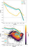 |
Fig. 2 [C/Fe] vs. [Fe/H] ratios for different models. Upper panel: [C/Fe] vs. [Fe/H] ratios as predicted by the one-infall model for different stellar yields and percentages of binaries (see legend). The thin gray dashed lines indicate the solar ratios. Lower panel: [C/Fe] vs. [Fe/H] ratios as predicted by the two-infall model for different stellar yields and compared with data from Nissen et al. (2020, white points) and APOGEE (Abdurro’uf etal. 2022). |
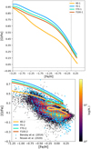 |
Fig. 3 [O/Fe] vs. [Fe/H] ratios for different models. Upper and lower panel are the same as in Fig. 2 but for [O/Fe]. Data are from Bensby et al. (2014, blue triangles), Nissen et al. (2020, white points) and APOGEE (Abdurro’uf et al. 2022, colored according to their number density; see the color bar). |
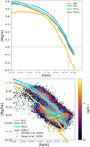 |
Fig. 4 [Mg/Fe] vs. [Fe/H] ratios for different models. Upper and lower panel are the same as in Fig. 2 but for [Mg/Fe]. Data are from Bensby et al. (2014, blue triangles), Nissen et al. (2020, white points) and APOGEE (Abdurro’uf et al. 2022, colored according to their number density; see color bar). |
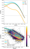 |
Fig. 5 [Ca/Fe] vs. [Fe/H] ratios for different models. Upper and lower panel are the same as in Fig. 2 but for [Ca/Fe]. Data are from Bensby et al. (2014, blue triangles), Nissen et al. (2020, white points) and (Abdurro’uf et al. 2022, colored according to their number density; see color bar). |
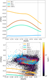 |
Fig. 6 [Ti/Fe] vs. [Fe/H] ratios for different models. Upper and lower panel are the same as in Fig. 2 but for [Ti/Fe]. Data are from Bensby et al. (2014, blue triangles), Nissen et al. (2020, white points) and Abdurro’uf et al. (2022, colored according to their number density; see color bar). |
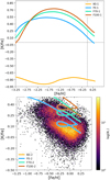 |
Fig. 7 [K/Fe] vs. [Fe/H] ratios for different models. Upper and lower panel are the same as in Fig. 2 but for [K/Fe]. Data are from Abdurro’uf et al. (2022, colored according to their number density; see color bar). |
4.2.2 Potassium
Moving now to odd-Z elements, we focus our attention on K, whose yields have been shown to severely underestimate the observed Galaxy abundance patterns (Romano et al. 2010; Kobayashi et al. 2020a and references therein), even when invoking mechanisms such as stellar rotation (Prantzos et al. 2018).
In Fig. 7, we compare results from our models for [K/Fe] versus [Fe/H], testing the newly proposed massive star yields by Farmer et al. (2023). In the upper panel, the difference between the various sets of yields is striking. On the one hand, the Reference Model K0-1 shows a very low ratio of [K/Fe] at all metallicities, ranging from ~−0.6 dex to ~−0.9 dex. On the other hand, the models adopting Farmer et al. (2023) yields show a very different pattern. From [Fe/H] ~−3.0 dex towards higher metallicities, all models show an important increase in the [K/Fe] ratio, which depends on the fraction of binaries assumed in the chemical evolution model. The highest increase is observed for models with higher binary fraction, starting from subsolar [K/Fe] ratios and reaching values of higher than 0.6 dex before the decline caused by the Type Ia SN contribution. Assuming no binaries instead, the chemical evolution track starts from slightly supersolar [K/Fe] ratios and reaches values of the order of 0.5 dex. Such different behaviors are due to the fact that in the Farmer et al. (2023) yield grids, very high-mass stars in binaries are producing a lower amount of K, while massive stars of lower mass (which dominate the global contribution towards higher metallicities) show more favorable conditions for K production relative to single stars in the same mass range. As suggested in Farmer et al. (2023), potassium is greatly affected by the binary star presence, with the main contributors to its production being low-mass binary-stripped stars during their pre-supernova evolution.
The radically different behavior between the Reference Model, representing what is generally predicted by the most used yield sets in the literature (Woosley & Weaver 1995; Kobayashi et al. 2006; Kobayashi & Nakasato 2011; Limongi & Chieffi 2018), and the models adopting Farmer et al. (2023) yields has important implications when comparing the results with the observed abundance patterns in the MW. This is shown in the lower panel of Fig. 7: while the Reference Model K0-2 falls even below the range of [K/Fe] values shown in the panel, the Model F0-2 (assuming Farmer et al. 2023 yields without binaries) reproduces the observed abundance trend in the solar vicinity very well. It is worth noting that this is the first time that chemical evolution models for the MW have been shown to reproduce the observed K trend without invoking ad hoc assumptions in the yields (see e.g., François et al. 2004). Instead, the models including massive binary-stripped star yields overestimate the observed [K/Fe] and this overestimation is proportional to the binary fraction.
4.2.3 Chromium
For what concerns the Fe-peak group, the element showing the most significant variations between different yield sets is Cr. In the upper panel of Fig. 8, we observe that the Reference Model K0-1 shows a rather flat, roughly solar pattern. The models adopting Farmer et al. (2023) yields with high binary fractions (F70-1 and F100-1) instead produce an increasing [Cr/Fe] ratio, with values starting from −0.2 dex (F100-1) and −0.4 dex (F70-1) and roughly reaching the solar ratio at [Fe/H]≳0. The F0-1 Model, on the other hand, shows an extremely low [Cr/Fe] ratio when compared to the other models at low metallicity ([Cr/Fe] ~−1.4 dex at [Fe/H] ~−3 dex) and a progressive increase towards larger metallicities, reaching [Cr/Fe] ~−0.15 dex at [Fe/H]≳0. This indicates that in the Farmer et al. (2023) stellar models, single massive stars are highly subdominant Cr producers relative to Fe. This is at variance with binary-stripped stars, where Cr is produced in similar amounts to Fe, as found in most of the available literature prescriptions (see also Prantzos et al. 2018; Kobayashi et al. 2020b; Palla 2021).
In the lower panel of Fig. 8, we can see that the roughly flat behavior shown by the Reference Model and the Farmer et al. (2023) model with the highest binary fraction (F100-2) well reproduce the trend of data from solar neighborhood stars presented in Sect. 3. The analysis of this panel excludes the Model F0-2 as a good tracer of chromium in the solar vicinity, as it predicts a [Cr/Fe] increasing trend that is not observed in APOGEE, Bensby et al. (2014), or Nissen et al. (2020) (see also Bergemann & Cescutti 2010; Adibekyan et al. 2012). For the remaining F70-2 Model, we see that its chemical tracks underestimate the observed Galactic Cr content, as seen in Bensby et al. (2014), especially for metallicities below [Fe/H] ≲ −0.5 dex. In conclusion, both the Reference Model and the F100-2 Model reproduce the general trend. However, we cannot draw firm conclusions as to which of the two is in better agreement with the observations. Furthermore, as the contribution of Type Ia SNe to Cr abundance is comparable to that of massive stars, different yield prescriptions for Type Ia SNe could change the chemical evolution picture (see Palla 2021 and references therein) in favor of one or the other model.
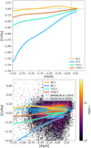 |
Fig. 8 [Cr/Fe] vs. [Fe/H] ratios for different models. Upper and lower panel are the same as in Fig. 2 but for [Cr/Fe]. Data from Bensby et al. (2014, blue triangles), Nissen et al. (2020, white points) and Abdurro’uf et al. (2022, colored according to their number density; see color bar). |
4.3 Discussion and caveats
In this study, we investigated the effects of the yields from massive single and binary-stripped stars computed by Farmer et al. (2023) on the simulated chemical evolution of the Galaxy. Previous studies (e.g., De Donder & Vanbeveren 2002) have explored the effects of the yields from massive interacting binaries, adopting a model similar to that of Chiappini et al. (1997) and therefore similar to the model we adopt here. The conclusions from these studies were that the inclusion of massive binaries in the Galactic chemical enrichment did not lead to striking differences, and the effects on the results were not larger than a factor of 2 relative to the evolution without binaries. The recent work of Farmer et al. (2023) has revived interest in studying the effects of chemical pollution from binary systems. This is because most of the massive stars in the Galaxy are likely to reside in binary systems (≳70%; e.g., De Rosa et al. 2014; Thies et al. 2015), as the vast majority of stars form as binaries and dynamical processes do not have the time to significantly decrease the binary fraction within the stellar lifetimes (Kroupa et al. 2024).
The present analysis shows that the adoption of yields for massive stars in binaries – as opposed to standard nucleosynthesis prescriptions from single massive stars – can lead to different solar abundances (e.g., Romano et al. 2010 and references therein), and for some elements they improve the agreement with observations. However, a shortcoming of the Farmer et al. (2023) yield grids is that they are computed – either for stars in single or binary systems – for a unique stellar chemical composition, namely the solar one. On the other hand, most of the yields from single massive stars present in the literature are computed for various chemical compositions, from absent (e.g. Heger & Woosley 2010) or very low metal content (e.g., [Fe/H]=−3 dex; Limongi & Chieffi 2018) up to the solar composition. This variation can create large differences and a fair comparison will only be possible when the yields for stars in massive interacting binaries have been computed for different metallicities; this is particularly important for elements with a prominent secondary component, such as 14N, the odd-Z elements27 Al and 23Na, and 63Cu. In particular, the evolution of partly secondary elements, such as 14N, can be quite different, as the yields are very low at low metallicity and therefore the overall element production is lower than when assuming the yield computed for the solar metallicity during the entirety of the chemical evolution, as is done in the present study.
Another limitation of the present work is related to the fate and yields of secondary stars in binaries, which are treated here as single stars. This is actually inherited from the study of Farmer et al. (2023), which does not provide the nucleosynthetic yields from such binary products. Their most significant contribution would likely be due to the mass gain, inducing stars that are initially too small to produce SNe (initial mass slightly lower than 8 M⊙) to gain enough mass to explode (e.g., Podsiadlowski et al. 2004; Zapartas et al. 2017, 2019). However, the picture is even more complex, as their contribution to the Galactic chemical enrichment also depends on: (i) the fraction of mass that they accreted and that remained bound and (ii) the amount of this accreted, bound mass that is further processed inside the secondary star (see e.g., Deckers et al. 2021).
Finally, another source of uncertainty in the yield computation is the adopted stellar evolution code. Different codes include different treatments of the physical processes (e.g., convection and SN-induced explosion) inside the stars and therefore produce different results.
Here, we therefore do not intend to draw firm conclusions regarding the effects of binaries on the chemical enrichment process; neither do we intend to establish the correct percentage of massive binaries, as we are also lacking well-sampled grids of binary system parameters, such as mass ratio and orbital period, and are restricted to those for which all massive binaries undergo case B mass transfer, producing binary-stripped primary stars (see Moe & Di Stefano 2017 for a review on binary parameter distribution). Rather, the goal of this paper is to indicate that the inclusion of yields from massive stars in binaries can affect the agreement between model results and observed abundances.
In this way, our study is designed to both (i) encourage further development in stellar yield modeling in binary systems, enlarging the grids in metallicities and binary system conditions, and (ii) to provide a basis for future studies investigating the influence of binary systems in terms of Galactic chemical evolution.
5 Conclusions
In this study, we have compared the results from detailed and well-tested chemical evolution models for the MW (e.g., Spitoni et al. 2019; Palla et al. 2020) including either yields from single massive stars or yields considering the contribution of massive stars in interacting binaries.
In particular, we tested the yields from massive binary-stripped stars as computed by Farmer et al. (2023) and assumed different binary fractions in the IMF, that is, from 0% to 100%. We also consider standard yields for single massive stars (Romano et al. 2010; i.e., our Reference Model) largely adopted in previous chemical evolution works to facilitate the comparison with what is obtained with available literature prescriptions. Our goal is to test whether the inclusion of the yields of massive stars in binaries could substantially change the modeled abundance patterns in the solar vicinity. It is worth noting that such results are relevant, as in the last two decades no other studies have addressed the effects of massive binary systems on the chemical evolution of the Galaxy (De Donder & Vanbeveren 2002).
Our key findings can be summarized as follows:
When adopting Farmer et al. (2023) stellar yields, the differences in the predictions obtained by varying the percentage of binary stars are negligible for a large fraction of the studied chemical elements;
A more marked difference is instead found for both the predicted solar abundances and the abundance patterns ([X/Fe] vs. [Fe/H]) between the Reference Model (K0-2) – adopting standard yields for single massive stars dependent on metallicity – and models adopting Farmer et al. (2023) stellar yields, which are for single massive stars at solar metallicity;
By adopting Farmer et al. (2023) yields for single stars (Model F0-2), the solar abundances predicted by the chemical evolution models are in better agreement with observations than those predicted by the Reference Model K0-2 for 4He, 12C, 14N, 24Mg, 39K, 40Ca, 55Mn, and 59Co. Of these elements, when considering [X/Fe] versus [Fe/H] diagrams, the [C/Fe] ratio as predicted by the F0-2 Model exhibits some difficulty in reproducing all the data, although it is in relatively good agreement with the findings of Nissen et al. (2020) and Abdurro’uf et al. (2022) for solar and supersolar metallicities. The [Mg/Fe] predicted ratio instead shows remarkable agreement with both the high-α and low-α sequence, which is not found with the yields adopted in the Reference Model, or with other yield prescriptions available in the literature (see Palla et al. 2022). Also, the predicted [Ca/Fe] versus [Fe/H] relation reproduces the observational data from all adopted samples very well, especially at high metallicity. Finally, the Model F0-2 is able to reproduce the observed 39K trend without invoking ad hoc assumptions regarding the yields, as are required by most of the available stellar yield prescriptions (e.g., Kobayashi et al. 2020a);
Regarding models that use the Farmer et al. (2023) yields with different fractions of binary systems, when comparing their predicted solar abundances to the Reference Model K0-2, we find that Model F70-2 (70% binary fraction) shows better agreement for 24Mg, 40Ca, and 56Fe, while F100-2 shows better results for 40Ca, 52Cr, and 56Fe than the Reference Model. For both [Ca/Fe] and [Mg/Fe], the inclusion of binary-stripped yields with different fractions produces a similar pattern to that resulting from the use of Farmer et al. (2023) yields with single stars only, thus allowing a good reproduction of the observed abundance patterns in the solar vicinity. Finally, the [Cr/Fe] ratio is best reproduced by F100-2, whereas F70-2 slightly underestimates the trend observed in Bensby et al. (2014);
Both the 16O predicted solar abundances and the [O/Fe] versus [Fe/H] relation are generally overestimated by all models, and especially by the F0-2 Model, which does not reproduce the observed data trend at all. On the other hand, the solar abundances and abundance patterns predicted by all models largely underestimate48 Ti, with the results of the Model F0-2 significantly increasing the already present discrepancy with the observed [Ti/Fe] data trend;
For the other chemical elements, we do not observe noticeable differences in the predicted solar abundances – or in the [X/Fe] versus [Fe/H] ratios – when comparing the results obtained with different yields. We also refrain from drawing conclusions regarding the abundance patterns of elements with relevant secondary production (e.g., 14N), as the new yields of Farmer et al. (2023) are currently only computed for solar metallicity, which prevents a fair comparison with other models and observations.
Acknowledgements
The authors want to thank the anonymous referee for the important and useful suggestions improving the manuscript content. MP acknowledges financial support from the project “LEGO – Reconstructing the building blocks of the Galaxy by chemical tagging” granted by the Italian MUR through contract PRIN2022LLP8TK_001. F. Matteucci thanks I.N.A.F. for the 1.05.12.06.05 Theory Grant – Galactic archaeology with radioactive and stable nuclei. F. Matteucci thanks also support from Project PRIN MUR 2022 (code 2022ARWP9C) “Early Formation and Evolution of Bulge and HalO (EFEBHO)” (PI: M. Marconi). E. Spitoni thanks I.N.A.F. for the 1.05.23.01.09 Large Grant – Beyond metallicity: Exploiting the full POtential of CHemical elements (EPOCH) (ref. Laura Magrini). In this work, we have made use of SDSS-IV APOGEE-2 DR17 data. Funding for the Sloan Digital Sky Survey IV has been provided by the Alfred P. Sloan Foundation, the U.S. Department of Energy Office of Science, and the Participating Institutions. SDSS-IV acknowledges support and resources from the Center for High-Performance Computing at the University of Utah. The SDSS web site is www.sdss.org. SDSS is managed by the Astrophysical Research Consortium for the Participating Institutions of the SDSS Collaboration which are listed at www.sdss.org/collaboration/affiliations/.
References
- Abdurro’uf, Accetta, K., Aerts, C., et al. 2022, ApJS, 259, 35 [NASA ADS] [CrossRef] [Google Scholar]
- Adibekyan, V. Z., Sousa, S. G., Santos, N. C., et al. 2012, A&A, 545, A32 [NASA ADS] [CrossRef] [EDP Sciences] [Google Scholar]
- Asplund, M., Grevesse, N., Sauval, A. J., & Scott, P. 2009, ARA&A, 47, 481 [NASA ADS] [CrossRef] [Google Scholar]
- Bensby, T., Feltzing, S., & Oey, M. S. 2014, A&A, 562, A71 [NASA ADS] [CrossRef] [EDP Sciences] [Google Scholar]
- Bergemann, M., & Cescutti, G. 2010, A&A, 522, A9 [NASA ADS] [CrossRef] [EDP Sciences] [Google Scholar]
- Boissier, S., & Prantzos, N. 1999, MNRAS, 307, 857 [NASA ADS] [CrossRef] [Google Scholar]
- Chiappini, C., Matteucci, F., & Gratton, R. 1997, ApJ, 477, 765 [Google Scholar]
- Chiosi, C. 1980, A&A, 83, 206 [NASA ADS] [Google Scholar]
- De Donder, E., & Vanbeveren, D. 2002, New Astron., 7, 55 [NASA ADS] [CrossRef] [Google Scholar]
- De Donder, E., & Vanbeveren, D. 2004, New Astron. Rev., 48, 861 [CrossRef] [Google Scholar]
- De Rosa, R. J., Patience, J., Wilson, P. A., et al. 2014, MNRAS, 437, 1216 [NASA ADS] [CrossRef] [Google Scholar]
- Deckers, M., Groh, J. H., Boian, I., & Farrell, E. J. 2021, MNRAS, 507, 3726 [NASA ADS] [CrossRef] [Google Scholar]
- Ekström, S., Meynet, G., Chiappini, C., Hirschi, R., & Maeder, A. 2008, A&A, 489, 685 [NASA ADS] [CrossRef] [EDP Sciences] [Google Scholar]
- Farmer, R., Laplace, E., de Mink, S. E., & Justham, S. 2021, ApJ, 923, 214 [NASA ADS] [CrossRef] [Google Scholar]
- Farmer, R., Laplace, E., Ma, J.-z., de Mink, S. E., & Justham, S. 2023, ApJ, 948, 111 [NASA ADS] [CrossRef] [Google Scholar]
- François, P., Matteucci, F., Cayrel, R., et al. 2004, A&A, 421, 613 [NASA ADS] [CrossRef] [EDP Sciences] [Google Scholar]
- Gaia Collaboration (Brown, A. G. A., et al.) 2016, A&A, 595, A2 [NASA ADS] [CrossRef] [EDP Sciences] [Google Scholar]
- Gaia Collaboration (Brown, A. G. A, et al.) 2021, A&A, 649, A1 [NASA ADS] [CrossRef] [EDP Sciences] [Google Scholar]
- García Pérez, A. E., Allende Prieto, C., Holtzman, J. A., et al. 2016, AJ, 151, 144 [Google Scholar]
- Greggio, L., & Renzini, A. 1983, A&A, 118, 217 [NASA ADS] [Google Scholar]
- Grevesse, N., & Sauval, A. J. 1998, Space Sci. Rev., 85, 161 [Google Scholar]
- Gunn, J. E., Siegmund, W. A., Mannery, E. J., et al. 2006, AJ, 131, 2332 [NASA ADS] [CrossRef] [Google Scholar]
- Gustafsson, B., Edvardsson, B., Eriksson, K., et al. 2008, A&A, 486, 951 [NASA ADS] [CrossRef] [EDP Sciences] [Google Scholar]
- Harris, J. A., Hix, W. R., Chertkow, M. A., et al. 2017, ApJ, 843, 2 [NASA ADS] [CrossRef] [Google Scholar]
- Hegedűs, V., Mészáros, S., Jofré, P., et al. 2023, A&A, 670, A107 [NASA ADS] [CrossRef] [EDP Sciences] [Google Scholar]
- Heger, A., & Woosley, S. E. 2010, ApJ, 724, 341 [Google Scholar]
- Hirschi, R. 2005, in From Lithium to Uranium: Elemental Tracers of Early Cosmic Evolution, 228, eds. V. Hill, P. Francois, & F. Primas, 331 [NASA ADS] [Google Scholar]
- Hirschi, R. 2007, A&A, 461, 571 [NASA ADS] [CrossRef] [EDP Sciences] [Google Scholar]
- Hopkins, P. F., Gurvich, A. B., Shen, X., et al. 2023, MNRAS, 525, 2241 [NASA ADS] [CrossRef] [Google Scholar]
- Iwamoto, K., Brachwitz, F., Nomoto, K., et al. 1999, ApJS, 125, 439 [NASA ADS] [CrossRef] [Google Scholar]
- Jermyn, A. S., Bauer, E. B., Schwab, J., et al. 2023, ApJS, 265, 15 [NASA ADS] [CrossRef] [Google Scholar]
- Jönsson, H., Holtzman, J. A., Allende Prieto, C., et al. 2020, AJ, 160, 120 [Google Scholar]
- Karakas, A. I. 2010, MNRAS, 403, 1413 [NASA ADS] [CrossRef] [Google Scholar]
- Kennicutt, Jr., R. C. 1998, ApJ, 498, 541 [Google Scholar]
- Kobayashi, C., & Nakasato, N. 2011, ApJ, 729, 16 [NASA ADS] [CrossRef] [Google Scholar]
- Kobayashi, C., Umeda, H., Nomoto, K., Tominaga, N., & Ohkubo, T. 2006, ApJ, 653, 1145 [NASA ADS] [CrossRef] [Google Scholar]
- Kobayashi, C., Karakas, A. I., & Lugaro, M. 2020a, ApJ, 900, 179 [Google Scholar]
- Kobayashi, C., Leung, S.-C., & Nomoto, K. 2020b, ApJ, 895, 138 [CrossRef] [Google Scholar]
- Kroupa, P., Tout, C. A., & Gilmore, G. 1993, MNRAS, 262, 545 [NASA ADS] [CrossRef] [Google Scholar]
- Kroupa, P., Gjergo, E., Jerabkova, T., & Yan, Z. 2024, arXiv e-prints [arXiv:2410.07311] [Google Scholar]
- Lada, C. J., & Lada, E. A. 2003, ARA&A, 41, 57 [Google Scholar]
- Langer, N. 2012, ARA&A, 50, 107 [CrossRef] [Google Scholar]
- Laplace, E., Götberg, Y., de Mink, S. E., Justham, S., & Farmer, R. 2020, A&A, 637, A6 [NASA ADS] [CrossRef] [EDP Sciences] [Google Scholar]
- Laplace, E., Justham, S., Renzo, M., et al. 2021, A&A, 656, A58 [NASA ADS] [CrossRef] [EDP Sciences] [Google Scholar]
- Leung, H. W., & Bovy, J. 2019, MNRAS, 489, 2079 [CrossRef] [Google Scholar]
- Limongi, M., & Chieffi, A. 2018, ApJS, 237, 13 [NASA ADS] [CrossRef] [Google Scholar]
- Magkotsios, G., Timmes, F. X., Hungerford, A. L., et al. 2010, ApJS, 191, 66 [NASA ADS] [CrossRef] [Google Scholar]
- Matteucci, F. 2012, Chemical Evolution of Galaxies [Google Scholar]
- Matteucci, F. 2021, A&A Rev., 29, 5 [NASA ADS] [CrossRef] [Google Scholar]
- Matteucci, F., & Francois, P. 1989, MNRAS, 239, 885 [Google Scholar]
- Matteucci, F., & Greggio, L. 1986, A&A, 154, 279 [NASA ADS] [Google Scholar]
- Matteucci, F., & Recchi, S. 2001, ApJ, 558, 351 [NASA ADS] [CrossRef] [Google Scholar]
- Melioli, C., Brighenti, F., D’Ercole, A., & de Gouveia Dal Pino, E. M. 2008, MNRAS, 388, 573 [Google Scholar]
- Melioli, C., Brighenti, F., D’Ercole, A., & de Gouveia Dal Pino, E. M. 2009, MNRAS, 399, 1089 [Google Scholar]
- Meynet, G., & Maeder, A. 2002, A&A, 390, 561 [NASA ADS] [CrossRef] [EDP Sciences] [Google Scholar]
- Moe, M., & Di Stefano, R. 2017, ApJS, 230, 15 [Google Scholar]
- Molero, M., Magrini, L., Matteucci, F., et al. 2023, MNRAS, 523, 2974 [NASA ADS] [CrossRef] [Google Scholar]
- Nissen, P. E., Christensen-Dalsgaard, J., Mosumgaard, J. R., et al. 2020, A&A, 640, A81 [NASA ADS] [CrossRef] [EDP Sciences] [Google Scholar]
- Nomoto, K., Kobayashi, C., & Tominaga, N. 2013, ARA&A, 51, 457 [CrossRef] [Google Scholar]
- Paczyński, B. 1967, Acta Astron., 17, 355 [NASA ADS] [Google Scholar]
- Palla, M. 2021, MNRAS, 503, 3216 [Google Scholar]
- Palla, M., Matteucci, F., Spitoni, E., Vincenzo, F., & Grisoni, V. 2020, MNRAS, 498, 1710 [Google Scholar]
- Palla, M., Santos-Peral, P., Recio-Blanco, A., & Matteucci, F. 2022, A&A, 663, A125 [NASA ADS] [CrossRef] [EDP Sciences] [Google Scholar]
- Paxton, B., Bildsten, L., Dotter, A., et al. 2011, ApJS, 192, 3 [Google Scholar]
- Paxton, B., Cantiello, M., Arras, P., et al. 2013, ApJS, 208, 4 [Google Scholar]
- Paxton, B., Marchant, P., Schwab, J., et al. 2015, ApJS, 220, 15 [Google Scholar]
- Paxton, B., Schwab, J., Bauer, E. B., et al. 2018, ApJS, 234, 34 [NASA ADS] [CrossRef] [Google Scholar]
- Paxton, B., Smolec, R., Schwab, J., et al. 2019, ApJS, 243, 10 [Google Scholar]
- Podsiadlowski, P., Langer, N., Poelarends, A. J. T., et al. 2004, ApJ, 612, 1044 [NASA ADS] [CrossRef] [Google Scholar]
- Prantzos, N., Abia, C., Limongi, M., Chieffi, A., & Cristallo, S. 2018, MNRAS, 476, 3432 [Google Scholar]
- Rauscher, T., Heger, A., Hoffman, R. D., & Woosley, S. E. 2002, ApJ, 576, 323 [Google Scholar]
- Romano, D. 2022, A&A Rev., 30, 7 [NASA ADS] [CrossRef] [Google Scholar]
- Romano, D., Karakas, A. I., Tosi, M., & Matteucci, F. 2010, A&A, 522, A32 [NASA ADS] [CrossRef] [EDP Sciences] [Google Scholar]
- Romano, D., Matteucci, F., Zhang, Z.-Y., Ivison, R. J., & Ventura, P. 2019, MNRAS, 490, 2838 [NASA ADS] [CrossRef] [Google Scholar]
- Sandoval, M. A., Hix, W. R., Messer, O. E. B., Lentz, E. J., & Harris, J. A. 2021, ApJ, 921, 113 [CrossRef] [Google Scholar]
- Smith, V. V., Bizyaev, D., Cunha, K., et al. 2021, AJ, 161, 254 [NASA ADS] [CrossRef] [Google Scholar]
- Spina, L., Magrini, L., & Cunha, K. 2022, Universe, 8, 87 [NASA ADS] [CrossRef] [Google Scholar]
- Spitoni, E., Recchi, S., & Matteucci, F. 2008, A&A, 484, 743 [NASA ADS] [CrossRef] [EDP Sciences] [Google Scholar]
- Spitoni, E., Matteucci, F., Recchi, S., Cescutti, G., & Pipino, A. 2009, A&A, 504, 87 [NASA ADS] [CrossRef] [EDP Sciences] [Google Scholar]
- Spitoni, E., Silva Aguirre, V., Matteucci, F., Calura, F., & Grisoni, V. 2019, A&A, 623, A60 [NASA ADS] [CrossRef] [EDP Sciences] [Google Scholar]
- Spitoni, E., Verma, K., Silva Aguirre, V., & Calura, F. 2020, A&A, 635, A58 [NASA ADS] [CrossRef] [EDP Sciences] [Google Scholar]
- Spitoni, E., Verma, K., Silva Aguirre, V., et al. 2021, A&A, 647, A73 [EDP Sciences] [Google Scholar]
- Spitoni, E., Matteucci, F., Gratton, R., et al. 2024, A&A, 690, A208 [NASA ADS] [CrossRef] [EDP Sciences] [Google Scholar]
- Thies, I., Pflamm-Altenburg, J., Kroupa, P., & Marks, M. 2015, ApJ, 800, 72 [NASA ADS] [CrossRef] [Google Scholar]
- Tinsley, B. M. 1980, ApJ, 241, 41 [NASA ADS] [CrossRef] [Google Scholar]
- Tominaga, N., Umeda, H., & Nomoto, K. 2007, ApJ, 660, 516 [NASA ADS] [CrossRef] [Google Scholar]
- van den Heuvel, E. P. J. 1969, AJ, 74, 1095 [NASA ADS] [CrossRef] [Google Scholar]
- Ventura, P., Dell’Agli, F., Tailo, M., et al. 2022, Universe, 8, 45 [NASA ADS] [CrossRef] [Google Scholar]
- Woosley, S. E. 2019, ApJ, 878, 49 [Google Scholar]
- Woosley, S. E., & Weaver, T. A. 1995, ApJS, 101, 181 [Google Scholar]
- Zapartas, E., de Mink, S. E., Izzard, R. G., et al. 2017, A&A, 601, A29 [NASA ADS] [CrossRef] [EDP Sciences] [Google Scholar]
- Zapartas, E., de Mink, S. E., Justham, S., et al. 2019, A&A, 631, A5 [NASA ADS] [CrossRef] [EDP Sciences] [Google Scholar]
[X/Y] = log(X/Y) − log(X⊙/Y⊙), where X and Y are the abundances of the object studied and X⊙ and Y⊙ are solar abundances.
Here, for the chemical thick and thin disk we refer to the high-α and low-α sequences observed in the MW disk.
The primary, evolving star in the binary system fills the Roche lobe for the first time after core-hydrogen exhaustion.
The production of an element is primary when it stems directly from the fusion of H and He. Conversely, a secondary production implies metal seeds already present at stellar birth.
All Tables
All Figures
|
Fig. 1 ∆log(X/H) ratios for different elements as predicted by the two-infall model for different stellar yields and percentage of binaries (see legend). The tin gray dashed line indicates the solar ratios as measured in Asplund et al. (2009), while the gray shaded region is the abundance uncertainty. |
| In the text | |
|
Fig. 2 [C/Fe] vs. [Fe/H] ratios for different models. Upper panel: [C/Fe] vs. [Fe/H] ratios as predicted by the one-infall model for different stellar yields and percentages of binaries (see legend). The thin gray dashed lines indicate the solar ratios. Lower panel: [C/Fe] vs. [Fe/H] ratios as predicted by the two-infall model for different stellar yields and compared with data from Nissen et al. (2020, white points) and APOGEE (Abdurro’uf etal. 2022). |
| In the text | |
|
Fig. 3 [O/Fe] vs. [Fe/H] ratios for different models. Upper and lower panel are the same as in Fig. 2 but for [O/Fe]. Data are from Bensby et al. (2014, blue triangles), Nissen et al. (2020, white points) and APOGEE (Abdurro’uf et al. 2022, colored according to their number density; see the color bar). |
| In the text | |
|
Fig. 4 [Mg/Fe] vs. [Fe/H] ratios for different models. Upper and lower panel are the same as in Fig. 2 but for [Mg/Fe]. Data are from Bensby et al. (2014, blue triangles), Nissen et al. (2020, white points) and APOGEE (Abdurro’uf et al. 2022, colored according to their number density; see color bar). |
| In the text | |
|
Fig. 5 [Ca/Fe] vs. [Fe/H] ratios for different models. Upper and lower panel are the same as in Fig. 2 but for [Ca/Fe]. Data are from Bensby et al. (2014, blue triangles), Nissen et al. (2020, white points) and (Abdurro’uf et al. 2022, colored according to their number density; see color bar). |
| In the text | |
|
Fig. 6 [Ti/Fe] vs. [Fe/H] ratios for different models. Upper and lower panel are the same as in Fig. 2 but for [Ti/Fe]. Data are from Bensby et al. (2014, blue triangles), Nissen et al. (2020, white points) and Abdurro’uf et al. (2022, colored according to their number density; see color bar). |
| In the text | |
|
Fig. 7 [K/Fe] vs. [Fe/H] ratios for different models. Upper and lower panel are the same as in Fig. 2 but for [K/Fe]. Data are from Abdurro’uf et al. (2022, colored according to their number density; see color bar). |
| In the text | |
|
Fig. 8 [Cr/Fe] vs. [Fe/H] ratios for different models. Upper and lower panel are the same as in Fig. 2 but for [Cr/Fe]. Data from Bensby et al. (2014, blue triangles), Nissen et al. (2020, white points) and Abdurro’uf et al. (2022, colored according to their number density; see color bar). |
| In the text | |
Current usage metrics show cumulative count of Article Views (full-text article views including HTML views, PDF and ePub downloads, according to the available data) and Abstracts Views on Vision4Press platform.
Data correspond to usage on the plateform after 2015. The current usage metrics is available 48-96 hours after online publication and is updated daily on week days.
Initial download of the metrics may take a while.