| Issue |
A&A
Volume 694, February 2025
|
|
|---|---|---|
| Article Number | A247 | |
| Number of page(s) | 8 | |
| Section | The Sun and the Heliosphere | |
| DOI | https://doi.org/10.1051/0004-6361/202452288 | |
| Published online | 19 February 2025 | |
Extended drag-based model for better predicting the evolution of coronal mass ejections
1
MIDA, Dipartimento di Matematica Università di Genova, Via Dodecaneso 35, 16146 Genova, Italy
2
Osservatorio Astrofisico di Torino, Istituto Nazionale di Astrofisica, Strada Osservatorio 20, 10025 Pino Torinese, Italy
⋆ Corresponding author; This email address is being protected from spambots. You need JavaScript enabled to view it.
Received:
17
September
2024
Accepted:
17
January
2025
Abstract
Coronal mass ejections (CMEs) are one of the primary drivers of space weather disturbances, affecting both space-based and terrestrial technologies. The accurate prediction of CME trajectories and their arrival times at Earth is crucial for mitigating potential impacts. In this work, we introduce an extended drag-based model (EDBM) that incorporates an additional acceleration term to better capture the complex dynamics of CMEs as they propagate through the heliosphere. Preliminary results suggest that the EDBM can improve upon the classical drag-based model by providing more reliable estimates of CME travel times, particularly in cases where the CME experiences residual acceleration. However, further validation is required to fully assess the operational potential of the model for space weather forecasting. This study lays the groundwork for future investigations and applications, with the aim of enhancing the accuracy of CME prediction models.
Key words: methods: analytical / methods: data analysis / Sun: coronal mass ejections (CMEs) / Sun: heliosphere / Sun: magnetic fields / solar wind
© The Authors 2025
 Open Access article, published by EDP Sciences, under the terms of the Creative Commons Attribution License (https://creativecommons.org/licenses/by/4.0), which permits unrestricted use, distribution, and reproduction in any medium, provided the original work is properly cited.
This article is published in open access under the Subscribe to Open model. This email address is being protected from spambots. You need JavaScript enabled to view it. to support open access publication.
1. Introduction
Coronal mass ejections (CMEs; Chen 2011; Howard 2011; Webb & Howard 2012; Gou et al. 2019) are massive outbursts of magnetized plasma from the solar corona into interplanetary space. When directed toward Earth, they cause severe geomagnetic disturbances (Gopalswamy 2016; Jin et al. 2016; Telloni et al. 2023; Guastavino et al. 2024) and can pose a persistent hazard as harmful radiation to space- and ground-based facilities, and human health. Therefore, predicting the CMEs’ arrival time and impact speed at Earth is essential in the context of the space weather forecasting science (Camporeale 2019).
One of the most popular and commonly used approaches to predict the transit time of a CME and its speed to Earth is known as the drag-based model (DBM) (e.g., Vršnak & Gopalswamy 2002; Vršnak et al. 2013; Hess & Zhang 2014; Napoletano et al. 2018; Dumbović et al. 2018; Kay & Gopalswamy 2018; Stamkos et al. 2023). This model assumes that the kinematics of the CME is governed by its dynamic interaction with the spiral-shaped Parker interplanetary structures (i.e., high- and low-speed streams) where it propagates, via the magnetohydrodynamic equivalent of the aerodynamic drag force. The model, which mathematically reduces to a rather simple equation of motion, thus essentially predicts that the speed of the CME will balance that of the ambient solar wind in which it is expanding. Recent efforts have also been devoted to incorporating the physics of aerodynamic drag into methodologies based on artificial intelligence (AI) techniques, paving the way for innovative (hybrid) approaches known as physics-driven AI models (Guastavino et al. 2023).
Although the DBM has been subject to continuous refinements (in this regard, it is worth mentioning the 3D Coronal Rope Ejection (3DCORE) developed by Möstl et al. 2018) and is now a well-established approach, several drawbacks associated with its intrinsic approximations are evident. Indeed, it is clear that the complex dynamical interaction of the CME with its surroundings cannot be properly described solely by the drag force. Other important physical processes are certainly at play in the evolution of CMEs: these include CME rotation, reconfiguration, deformation, deflection, and erosion, along with any other magnetic reconnection-driven process (see the review by Manchester et al. 2017, for a rather comprehensive dissertation on this topic), resulting in additional accelerations beyond that predicted by the trivial DBM acting on the CME as it travels through the heliosphere.
Regnault et al. (2024) recently pointed out that the DBM is often quite ineffective in describing the proper propagation of CMEs in interplanetary space. In this study, a CME was observed by two radially aligned probes separated by a distance of just 0.13 AU; namely, the Solar Orbiter (SolO) and Wind spacecraft. Although the model predicted that the CME would decelerate, the velocity profiles measured by the two spacecraft instead revealed a residual acceleration, pointing to an additional force to the drag that overpowered its braking effect, and thus resulting in an increase in velocity. This work presents a more refined and realistic DBM, with the aim being to overcome the limitations of current versions by introducing into the equation of motion describing the dynamic interaction of the CME with the solar wind an extra acceleration, representing any other forces involved.
After obtaining and discussing the mathematical solutions of the resulting new equations of motion (Sect. 2), the updated version is applied to the observation of the same CME already studied in Regnault et al. (2024), showing that it satisfactorily succeeds in describing its dynamic evolution, and thus becoming a significant breakthrough in the prediction of CME travel time in space weather studies (Sect. 3.). An interpretation of which physical process(es) the additional acceleration results from is tentatively given in Sect. 4, where our conclusions are also offered. Computational details on derived formulae in Sect. 2 are summarized in the appendix.
2. The extended drag-based model
We propose a generalization of the classical DBM to include an additional acceleration term, accounting for forces beyond drag, where the total net acceleration acting on the CME in the interplanetary phase is made of two contributions:
 (1)
(1)
where  , k ∈ 2ℕ + 1, and aextra = ar−β, for appropriate exponents, α, β > 0, and coefficients, γ > 0, a ≠ 0; r = r(t) and v(t) = ṙ(t) are the CME instantaneous radial position and speed (typically the CME front distance and front speed); and w(r, t) is the background solar wind speed given as a known function of position and time. Physically, the model describes the same dynamics of the DBM perturbed by an extra (e.g., magneto-gravitational) force acting on the CME along the motion, altogether exponentially damped over distance.
This generalization represents the simplest and most natural extension of the original DBM. In this framework, an additional acceleration term is introduced to account for forces beyond the drag interaction with the solar wind, such as magneto-gravitational forces or other external influences acting on the CME. Moreover, this is the only way to retain a form that allows for analytical treatment of the model, at least in simplified cases. This formulation ensures that both drag and non-drag forces are considered, while still preserving the mathematical structure necessary for deriving a closed-form solution under certain assumptions, as is discussed below.
In general, Eq. (1) does not admit an analytical solution, which hampers the computation of aextra from time and space measurements; that is, by solving a boundary value problem. A closed-form time solution of Eq. (1) is possible by assuming α = β = 0 and a constant w(r, t)≡w, for any fixed odd integer k (for more details on the original DBM, see Vršnak et al. (2013) and Cargill (2004)). Therefore, we introduced the extended DBM (EDBM hereafter) as the equation
 (2)
(2)
in which k = 1, and which corresponds to a straightforward perturbation of the simplest form of the DBM studied in Vršnak et al. (2013). The sign of a ≠ 0 in Eq. (2) establishes the form of the solution and the properties of the associated dynamical system.
We started from the equilibria:
-
if a < 0,
 is an asymptotically stable (in the future) constant solution of Eq. (2); thus, for
  (
( ) the CME monotonically decelerates (accelerates) for positive times;
 -
if a > 0,
 is an asymptotically stable (in the future) constant solution of Eq. (2); thus, for
  (
( ) the CME monotonically decelerates (accelerates) for positive times.
These assertions clarify the role of the acceleration term a ≠ 0: it shifts the asymptotic solution from v = w (standard DBM) to  (EDBM). In contrast to the case a = 0, this means that for a > 0 (a < 0) initial speeds below (above) the wind speed can increase (decrease) up (down) to w and beyond. A schematic of the dynamics around the equilibrium points is provided in Fig. 1.
 |
Fig. 1. Graphical representation of F(v)≔ − γ|v − w|(v − w)+a and local portrait of the speed dynamics around the stable equilibrium of the EDBM in the cases a < 0 and a > 0. The arrows define the positive sense of time for the evolution of v(t). Solid and dashed lines correspond to F > 0 (graph above the line, arrow pointing to the right) and F < 0 (graph below the line, arrow pointing to the left), respectively. |
Equation (2) can be integrated from 0 to t > 0 to obtain explicit formulae for v(t) and r(t), given the initial conditions v(0) = v0, r(0) = r0. Depending on the choice of v0, the solutions can be (differentially) piecewise-defined for positive or negative values of a due to the presence of the absolute value term |ṙ − w|, and present obvious symmetries in the form. Specifically,
Casea > 0:
-
if v0 ≤ w, then
 (3)
(3) (4)
(4)where
 and
and  ;
; -
if v0 > w, then
 (5)
(5) (6)
(6)where
 and
and  .
.
Casea < 0:
-
if v0 ≤ w, then
 (7)
(7) (8)
(8)where
 and
and  ;
; -
if v0 > w, then
 (9)
(9) (10)
(10)where
 and
and  .
.
The expressions for the CME speed reflect the dynamical behavior of Fig. 1. In Eq. (3), v(t)≤w in the former expression, while v(t) > w in the latter, and  as t → +∞. In Eq. (5), v(t) > w with
  as t → +∞, and v(t) is never smaller than or equal to w for positive times. In Eq. (7), v(t)≤w with
  as t → +∞, and v(t) is never larger than or equal to w for positive times. Finally, in Eq. (9), v(t)≥w in the former expression, while v(t) < w in the latter, and
  as t → +∞. The derivation of Eqs. (3)–(10) requires standard calculus techniques, whose details are given in Appendix A.
3. Proof of concept for the EDBM: Application to the November 3–5, 2021, event
As is discussed in Sect. 1, the closely spaced SolO-Wind detections of a CME of early November 2021 provided a reliable test case in which to assess the effectiveness of the EDBM. Indeed, in agreement with the analysis of Regnault et al. (2024), the wind speed profiles measured by SolO and Wind (Fig. 2) suggested an acceleration of the CME magnetic cloud (MC) front from SolO to Wind (bottom panel) rather than the expected deceleration due to the drag force induced by the background solar wind. Regarding the angular separation between SolO and Wind, we note that the spacecraft were located within 2.2° of each other in heliospheric longitude at the time of the CME passage. While this might imply that the two spacecraft are sampling slightly different CME portions, we argue that this small angular offset becomes less significant in light of the CME’s large-scale expansion as it propagates through the heliosphere. By the time CMEs reach 1 AU, they often expand radially to around 0.25 AU (Klein & Burlaga 1982), making a 2.2° difference quite minor relative to the overall CME structure. In this context, we assume that the spacecraft sample closely related plasma regions within the CME, a reasonable assumption supported by common practice in heliospheric studies. Aligning spacecraft at similar heliospheric longitudes is a well-established method of studying the radial evolution of CME structures. Several studies have effectively employed this approach, demonstrating that minor angular separations do not significantly impact the ability to observe the large-scale, radial evolution of CMEs. For instance, multi-spacecraft observations with small angular offsets were successfully used in studies by Skoug et al. (2000), Du et al. (2007), Nakwacki et al. (2011), Li et al. (2017), and Telloni et al. (2020). These works support the inference that small angular separations enable the CME’s large-scale evolution to be viewed consistently. While Regnault et al. (2024) attribute observed CME-related plasma flow differences to spatial variations caused by this angular separation, our model’s additional acceleration term suggests that these discrepancies can instead be reconciled when accounting for a full spectrum of forces beyond simple drag. Therefore, while we acknowledge that the spacecraft are likely observing slightly different CME segments due to the 2.2° longitudinal separation, our model demonstrates that by considering additional forces beyond drag, we can achieve a more accurate description of the CME’s behavior across multiple spacecraft, reducing discrepancies attributed to just angular separation. Hence, this small geometric uncertainty does not significantly affect the plasma flow measurements or the velocity profiles considered in our analysis. The transit times were adjusted based on each spacecraft’s specific radial position relative to the Sun, ensuring that the observed discrepancies between predicted and measured CME velocities result from dynamic factors rather than geometric projection effects. Although the physical reasons for this local behavior remain unclear (plausible interpretations are discussed in Sect. 4), in the following we applied the extended model described in Sect. 2 against data collected at SolO and Wind locations, rSolO and rWind, respectively, to estimate the additive acceleration, a > 0, between the two instruments. Specifically, given the measured MC front speeds, vSolO, vWind, at times tSolO, tWind, respectively, we focused on the difference between the mean acceleration,
 (11)
(11)
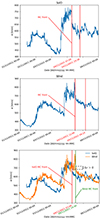 |
Fig. 2. Time series of the ambient solar wind from November 1 to November 6 (UT) measured by the Solar Orbiter Solar Wind Analyser (SWA) (top panel), by the Wind spacecraft (middle panel), and the two spacecraft combined (bottom panel). MC front limits are traced following Regnault et al. (2024) and Δv is defined as in (11). |
which is an indicator of the approximate total measured acceleration exerted on the CME between the two spacecraft, and the model-dependent acceleration contributions, adrag(SolO)+a and adrag(Wind)+a, where
 (12)
(12)
 (13)
(13)
We used the boundaries of the MC defined by Regnault et al. (2024) to maintain consistency between our work and their study. This decision ensures that our comparison of the models remains valid and directly addresses the discrepancies observed in their analysis. The boundaries, while subjective, are necessary to demonstrate the specific improvements introduced by the additional acceleration term in the EDBM. Changing the boundary selection would introduce other variables, potentially weakening the direct comparison that we aim to establish between our approach and their findings. To ensure a controlled, direct comparison with Regnault et al. (2024), we maintained the same boundary selection and γ parameter values that they employed. This alignment is crucial for isolating the improvements offered by the EDBM specifically in relation to the discrepancies they observed. By preserving these conditions, we minimized the introduction of additional variables that could complicate interpretation and obscure the specific contributions of the added acceleration term in the EDBM. While considerably varying CME boundaries or γ parameters could certainly expand the scope of our analysis, such changes would introduce further uncertainties that may interfere with this study’s primary goal. Here, our aim is to highlight how the EDBM effectively addresses previously noted limitations of the classical DBM. However, we acknowledge that investigating the robustness of the EDBM across a wide range of events and parameter values could offer a more comprehensive validation of its applicability. For this reason, we propose a preliminary investigation in this direction at the end of the present section, by slightly changing the quantities vSolO, vWind, and γ. Future studies will therefore explore how variations in all input parameters affect model performance to fully characterize the EDBM’s predictive capabilities.
The main task, therefore, was to determine, from the solutions, v(t),r(t), in Sect. 2, the values of the extra-acceleration term, a, that are compatible with the set of boundary values,
obtained from the data time series at the initial time, tSolO = 0, and final time, tWind = 17820 s, and the parameters (γ, w). More specifically, we considered several experiments by choosing w ∈ [400, 800] km/s with the incremental step Δw = 50 km/s, and we used the same value γ = 0.24 × 10⁻⁷ km−1, as in Regnault et al. (2024) (thus ensuring consistency and a fair comparison with their results, upon which our study builds, while allowing us to assess the improvements offered by our model, which introduces an additional acceleration term). This value of γ is compatible with the CME that erupted on November 2, 2021, at 02:48 UT and that was detected by the Solar and Heliospheric Observatory (SOHO) Large Angle and Spectrometric Coronagraph (LASCO) C2 (see, e.g., Li et al. 2022). The choice of this wide range of values is motivated by the fact that the MC is immersed in a nonconstant solar wind; that is, it lies at the interface between a high- and a low-speed stream. Downstream, the ambient solar wind speed is about 550 − 700 km/s (at 1 AU), while upstream it is about 400 − 500 km/s (at 1 AU). Therefore, by considering this range of solar wind speeds, we are able to model the CME propagation more accurately, acknowledging the variability and nonstationary nature of the solar wind. This approach also offers the opportunity to observe how the extra-acceleration term depends on the background wind speed. Through a standard root-finding Newton-Raphson method (Süli & Mayers 2003), for every w one has to search for the solution(s) (if any) of
 (14)
(14)
or
 (15)
(15)
using formulae (3)–(6) (case a > 0). We initialized the root-finding algorithm with an initial guess of approximately the same order of magnitude of |adrag(SolO)|, |adrag(Wind)|, and iterated until convergence to a local positive value (if the scheme did not converge, we would set a = 0).
For the sake of simplicity, we applied this scheme to Eq. (14) and, since formula (3) is case-defined and the time intervals depend on the unknown a, we eventually checked that for each experiment the corresponding time condition was fulfilled once a was found (if the time condition did not apply, we would reject the solution).
Figure 3 contains the results of this analysis. Specifically, in the topmost panel a positive extra-acceleration, a, was obtained for each choice of w (cyan curve), as opposed to a drag deceleration at SolO and Wind until w = 700 km/s (orange and green curves). The sum of the corresponding contributions provided two profiles that symmetrically fit the constant value amean in Eq. (11) with a notable degree of accuracy, independently of the ambient solar wind (from the magnification in the second panel from top, the maximum error committed is about 0.1 m/s2 attained at w = 400 km/s). Furthermore, it is worth mentioning the optimality that is reached at w = 700 km/s, with almost an exact match between the three accelerations. However, we recognize that a background solar wind speed of 650 km/s, which is more consistent with the downstream in situ observations, also provides an excellent fit. The 700 km/s value reflects a mathematical estimate required to match the total acceleration empirically derived from the CME travel time between SolO and Wind, while 650 km/s aligns more closely with the actual in situ measurements, even if exclusively downstream of the CME. 700 km/s is indeed the value for the solar wind numerically closest to vSolO and vWind.
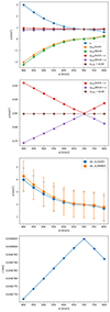 |
Fig. 3. Modeling the November 3–5, 2021, event with the EDBM. First panel from top: Extra-acceleration term predicted by the EDBM (cyan line) added to the acceleration terms predicted by the DBM at SolO (orange line) and Wind (green line) to obtain the red and purple lines that are compared to the experimental average acceleration from SolO to Wind (brown line). Second panel: Zoom on the experimental average and predicted accelerations. Third panel: Mean acceleration and corresponding standard deviation provided by the EDBM for ten random realizations of the initial and final speeds (blue and orange lines, respectively). Fourth panel: Absolute error, ε = |fr(a)|, from Eq. (15) at Wind for the EDBM solutions, a, obtained as in the topmost panel using Eq. (14). |
The last two panels from the top of the same figure describe the outcomes of two further tests. First, we generated two sets containing ten values of the extra-acceleration, a, computed for two sets of ten random realizations of the initial speed in the range [vSolO − 50, vSolO + 10] km/s and of the final speed in the range [vWind − 10, vWind + 50] km/s, respectively (the reason for this choice of ranges is twofold: it guarantees that vSolO < vWind, and a maximum error of 50 km/s is plausible, while accounting for the uncertainty on the temporal location of the MC boundary). It is worth noting that these intervals are not meant to capture the full range of possible MC front speeds but are instead used to derive an experimental uncertainty associated with the additional acceleration term we have introduced in our model. This step is crucial to quantify the uncertainties in our results, which are driven by the potential variations in boundary placement, not by the overall range of solar wind speeds observed in situ. The third panel from the top contains average values ⟨a⟩ and the corresponding standard deviations, σv(SolO),σv(Wind), computed over the two sets (these standard deviations stabilize after ten random realizations of the initial and final speeds). We note that σv(SolO)≈σv(Wind)≈1 m/s2 independently of w, and we coherently re-obtained the best agreement between the two profiles for w = 700 km/s. Second, in the bottom panel of Fig. 3, we computed the absolute error, ε = |fr(a)|, from Eq. (15) at Wind’s location for the solutions, a, obtained as in the topmost panel using Eq. (14). The overall error as a function of w did not exceed ε = 0.046805 AU (relative error ≈5%), attained at w = 700 km/s. We note that for this value of the wind speed, we found, at the same time, the best outcome as far as a is concerned, though the largest error on r. This suggests that a trade-off strategy is being relied on when fitting the real data either with the v(t) model (Eq. (14)) or the r(t) model (Eq. (15)).
The γ parameter directly influences the results of the EDBM and, as for the MC boundaries, is subject to uncertainties in the way it is usually estimated. Although a complete sensitivity analysis of the EDBM is beyond the scope of the present study, a preliminary test of its robustness is given by implementing different values of γ. Therefore, we repeated the experiment in the topmost panel of Fig. 3 by varying γ, keeping the same order of magnitude of the value used in Regnault et al. (2024). The results are presented in Fig. 4. We do not find significant qualitative changes comparing these outcomes with the previous experiment in Fig. 3, and the accuracy level of the fit around w = 650 km/s is preserved for each case considered. This evidence, and the above statistical performance for the MC boundaries in the third panel from the top of Fig. 3, shows that the EDBM provides a reliable response under small measurement uncertainties.
In this respect, we infer that the EDBM can accurately describe the dynamics of a vast sample of interplanetary CMEs, especially of those excluded by the simplest form of the DBM, like the ones propelled beyond the solar wind speed (case with w = 700 km/s in Fig. 3). Indeed, when w = 700 km/s is assumed, the intermediate condition, vSolO < w < vWind, holds, which cannot be modeled using the classical DBM (see Sect. 2).
It is important to emphasize that the analysis presented in this section represents a proof of concept rather than a full validation of the EDBM. The chosen event (November 3–5, 2021) serves as a case study to illustrate the potential of the EDBM in capturing the dynamics of CME propagation by incorporating additional forces beyond the classical drag. A single-event analysis does not offer comprehensive validation; thus, future work will involve applying the model to a broader set of events to ensure robustness and generalizability. This future validation will also incorporate standard forecasting metrics and statistical assessments to fully evaluate the model’s predictive capabilities across various interplanetary CME events.
4. Discussion and conclusions
As CMEs travel through interplanetary space, they can experience residual acceleration during their expansion due to several factors beyond solar wind drag. These include:
-
Magnetic forces: CMEs are highly magnetized plasma structures that carry their own magnetic field. As they expand into interplanetary space, their magnetic field interacts with the Sun’s interplanetary magnetic field. This interaction can generate magnetic forces that can lead to residual acceleration, depending on the alignment and strength of the magnetic fields. The magnetic pressure from the Sun’s field, which decreases with distance, may provide a residual push on the CME as it expands (e.g., Kilpua et al. 2017).
-
Pressure gradients: as CMEs move away from the Sun, they encounter regions of lower density and pressure. The difference between the internal pressure of the CME and the external pressure of the surrounding solar wind can cause the CME to continue expanding and accelerate. If the internal pressure of the CME remains higher than the external pressure for an extended period, this imbalance can drive residual acceleration during the CME’s expansion (e.g., Manchester et al. 2017).
-
Internal magnetic reconfiguration: the internal dynamics of a CME, including its magnetic tension forces and plasma flows, can also contribute to residual acceleration. Indeed, CMEs contain complex magnetic structures that can undergo reconfiguration or magnetic reconnection as they expand. These internal processes can release energy, contributing to the acceleration of the CME. For example, if magnetic loops within the CME reconnect, the release of magnetic energy could provide a push that accelerates the CME further into space (e.g., Yan et al. 2018).
-
Gravitational forces: although relatively weak at large distances from the Sun, gravitational forces from the Sun can still play a role. Near the Sun, gravity decelerates the CME, but as it moves farther away, the influence of gravity decreases. If the CME has not yet reached a terminal velocity, the reduction in gravitational influence can result in a relative acceleration as the opposing force weakens (e.g., Shen et al. 2012).
-
Plasma and magnetic pressure balance: the expansion of the CME involves the balance between plasma pressure and magnetic pressure within the CME and in the surrounding solar wind. As the CME expands and its internal pressure decreases, the balance between these pressures can change, leading to further acceleration. If the magnetic pressure within the CME remains relatively high, it could continue to push the CME outward (e.g., Wolfson & Saran 1998).
In general, these factors certainly contribute to the complex dynamics of CMEs as they travel through space, influencing their speed and trajectory beyond the initial influence of the solar wind. More specifically, the present study shows that the combination of these effects can be modeled by an extra-acceleration term that, when added to the drag force, contributes to explain the observations of a CME performed by SolO and Wind much more reliably than the standard DBM.
Understanding the processes itemized above is essential for predicting the behavior of CMEs and their potential impact on space weather and Earth’s environment. Disentangling which of these processes is currently at work in the evolution of CME under studio needs further analysis that, as it is beyond the scope of the present work, is left to a future paper. In future work, the EDMB could be integrated into near-real-time forecasting systems by building on the AI approaches outlined in Guastavino et al. (2023), in which the classical DBM is incorporated into neural network architectures for CME transit time estimation. The benefit is twofold: on the one hand, it is possible to consider physical processes underlying the interaction of CMEs with interplanetary structures in addition to the ones related to the drag force exerted by the solar wind, and on the other hand, it is possible to incorporate this model into the loss function of AI procedures as it has an analytical form. Specifically, the EDBM would be incorporated into a two-stage neural network model without the immediate requirement for simultaneous multi-spacecraft data: the first neural network would estimate the total acceleration (including both the drag and additional components), while the second network would use this estimated total acceleration to predict the CME’s transit time. This approach would enhance the forecasting capabilities of the model and allow for more accurate predictions of CME arrival times at Earth.
Acknowledgments
SG was supported by the Programma Operativo Nazionale (PON) “Ricerca e Innovazione” 2014-2020. All authors acknowledge the support of the Fondazione Compagnia di San Paolo within the framework of the Artificial Intelligence Call for Proposals, AIxtreme project (ID Rol: 71708). AMM is also grateful to the HORIZON Europe ARCAFF Project, Grant No. 101082164. SG, MP and AMM are also grateful to the Gruppo Nazionale per il Calcolo Scientifico - Istituto Nazionale di Alta Matematica (GNCS – INdAM). MR is also grateful to the Gruppo Nazionale per la Fisica Matematica – Istituto Nazionale di Alta Matematica (GNFM – INdAM).
References
- Camporeale, E. 2019, Space Weather, 17, 1166 [CrossRef] [Google Scholar]
- Cargill, P. J. 2004, Sol. Phys., 221, 135 [Google Scholar]
- Chen, P. F. 2011, Liv. Rev. Sol. Phys., 8, 1 [Google Scholar]
- Du, D., Wang, C., & Hu, Q. 2007, J. Geophys. Res.: Space Phys., 112, A09101 [NASA ADS] [CrossRef] [Google Scholar]
- Dumbović, M., Čalogović, J., Vršnak, B., et al. 2018, ApJ, 854, 180 [CrossRef] [Google Scholar]
- Gopalswamy, N. 2016, Geosci. Lett., 3, 8 [NASA ADS] [CrossRef] [Google Scholar]
- Gou, T., Liu, R., Kliem, B., Wang, Y., & Veronig, A. M. 2019, Sci. Adv., 5, 7004 [Google Scholar]
- Guastavino, S., Candiani, V., Bemporad, A., et al. 2023, ApJ, 954, 151 [NASA ADS] [CrossRef] [Google Scholar]
- Guastavino, S., Bahamazava, K., Perracchione, E., et al. 2024, ApJ, 971, 94 [Google Scholar]
- Hess, P., & Zhang, J. 2014, ApJ, 792, 49 [NASA ADS] [CrossRef] [Google Scholar]
- Howard, T. 2011, Coronal Mass Ejections: An Introduction (Springer Science& Business Media), 376 [CrossRef] [Google Scholar]
- Jin, M., Schrijver, C. J., Cheung, M. C. M., et al. 2016, ApJ, 820, 16 [NASA ADS] [CrossRef] [Google Scholar]
- Kay, C., & Gopalswamy, N. 2018, JGR, 123, 7220 [NASA ADS] [Google Scholar]
- Kilpua, E. K. J., Balogh, A., von Steiger, R., & Liu, Y. D. 2017, SSRv, 212, 1271 [NASA ADS] [Google Scholar]
- Klein, L., & Burlaga, L. 1982, J. Geophys. Res.: Space Phys., 87, 613 [NASA ADS] [CrossRef] [Google Scholar]
- Li, H., Wang, C., Richardson, J. D., & Tu, C. 2017, ApJ, 851, L2 [NASA ADS] [CrossRef] [Google Scholar]
- Li, X., Wang, Y., Guo, J., & Lyu, S. 2022, ApJ, 928, L6 [NASA ADS] [CrossRef] [Google Scholar]
- Manchester, W., Kilpua, E. K. J., Liu, Y. D., et al. 2017, SSRv, 212, 1159 [NASA ADS] [Google Scholar]
- Möstl, C., Amerstorfer, T., Palmerio, E., et al. 2018, SpWea, 16, 216 [Google Scholar]
- Nakwacki, M. S., Dasso, S., Démoulin, P., Mandrini, C. H., & Gulisano, A. M. 2011, A&A, 535, A52 [NASA ADS] [CrossRef] [EDP Sciences] [Google Scholar]
- Napoletano, G., Forte, R., Del Moro, D., et al. 2018, J. Space Weather Space Clim., 8, A11 [NASA ADS] [CrossRef] [EDP Sciences] [Google Scholar]
- Regnault, F., Al-Haddad, N., Lugaz, N., et al. 2024, ApJ, 962, 190 [Google Scholar]
- Shen, F., Wu, S. T., Feng, X., & Wu, C.-C. 2012, JGR, 117, A11101 [Google Scholar]
- Skoug, R. M., Feldman, W., Gosling, J., et al. 2000, J. Geophys. Res.: Space Phys., 105, 27269 [NASA ADS] [CrossRef] [Google Scholar]
- Stamkos, S., Patsourakos, S., Vourlidas, A., & Daglis, I. A. 2023, Sol. Phys., 298, 88 [NASA ADS] [CrossRef] [Google Scholar]
- Süli, E., & Mayers, D. F. 2003, An Introduction to Numerical Analysis (Cambridge University Press) [CrossRef] [Google Scholar]
- Telloni, D., Zhao, L., Zank, G. P., et al. 2020, ApJ, 905, L12 [NASA ADS] [CrossRef] [Google Scholar]
- Telloni, D., Schiavo, M. L., Magli, E., et al. 2023, ApJ, 952, 111 [NASA ADS] [CrossRef] [Google Scholar]
- Vršnak, B., & Gopalswamy, N. 2002, JGRA, 107, 1019 [Google Scholar]
- Vršnak, B., Žic, T., Vrbanec, D., et al. 2013, Sol. phys., 285, 295 [CrossRef] [Google Scholar]
- Webb, D. F., & Howard, T. A. 2012, LRSP, 9, 3 [NASA ADS] [Google Scholar]
- Wolfson, R., & Saran, S. 1998, ApJ, 499, 496 [NASA ADS] [CrossRef] [Google Scholar]
- Yan, X. L., Yang, L. H., Xue, Z. K., et al. 2018, ApJ, 853, L18 [Google Scholar]
Appendix A: Computation of the solutions of the EDBM
A.1. v0, v ≤ w
Assume to integrate (2) in [0, t] such that v0, v(t)≤w:
Distinguishing between a > 0 and a < 0, we obtain two different primitives for the left-hand side and get
now solving for v in both the expressions and setting v(t)≤w yield formulae (3) in the case  and (7).
As regards r(t), for a > 0, a second integration provides
using  . In the interval
 ![Mathematical equation: $ [0,\arctan(\sqrt{\gamma/a}(w-v_0))/\sqrt{a\gamma}] $](/articles/aa/full_html/2025/02/aa52288-24/aa52288-24-eq42.gif) the cosine is positive, so we can remove the absolute value and obtain Eq. (4) (first case).
the cosine is positive, so we can remove the absolute value and obtain Eq. (4) (first case).
For a < 0, we conveniently set  ,
,  and
and  . We have
where the integral is first computed by splitting the fraction as

and then performing the two subsequent (monotonic) changes of variable u = Aexp(Ct′) − B and U = 1 + B/u. Again, we can disregard the absolute value for t ≥ 0, and replacing back the values of A, B, C we get (8).
A.2. v0, v ≥ w
The procedure is the same as in Appendix A.1. Since now the integration of (2) reads
formulas derived for v(t) and r(t) are simply swapped for a ≶ 0. Upon substituting a ↦ −a,  or the other way around depending on the sign of a, an analogous argument for time intervals, absolute values, and a corresponding re-definition of constants A, B, C hold. This leads to Eqs. (5) (a > 0), (9) (first case, a < 0) for v(t), and (6) (a > 0), (10) (first case, a < 0) for r(t).
A.3. v0 < w < v
This time the integration of the EDBM gives rise to two contributions:
in addition, from Fig. 1, the forward dynamics rules out the case a < 0 (it is possible only backward in time) and requires  to arrive at v(t) > w (cf. Appendix A.1). Then, we have
which is the case of Appendix A.2 with lower limit of integration equal to w. So, upon solving for v, we obtain expression (3) in the case t > t*.
Concerning r(t), we need to integrate Eq. (3) (second case) from t* to t:
with r* = r(t*),  , B ≔ −1,
  . This relationship is formally identical to the one of r(t) in Appendix A.1, case a < 0. We find
Lastly, we determine r* by enforcing continuity at t = t* with the former expression in (4):
hence, replacing back in the expression of r(t), we retrieve the latter of (4).
A.4. v < w < v0
Following Appendix A.3, an analogous reasoning is applied in the case a < 0. The corresponding sign adaptation of quantities involving a (see Appendix A.2) and the continuity requirement with the first relationship of Eq. (10) produce formulae (9), (10) for  .
.
All Figures
|
Fig. 1. Graphical representation of F(v)≔ − γ|v − w|(v − w)+a and local portrait of the speed dynamics around the stable equilibrium of the EDBM in the cases a < 0 and a > 0. The arrows define the positive sense of time for the evolution of v(t). Solid and dashed lines correspond to F > 0 (graph above the line, arrow pointing to the right) and F < 0 (graph below the line, arrow pointing to the left), respectively. |
| In the text | |
|
Fig. 2. Time series of the ambient solar wind from November 1 to November 6 (UT) measured by the Solar Orbiter Solar Wind Analyser (SWA) (top panel), by the Wind spacecraft (middle panel), and the two spacecraft combined (bottom panel). MC front limits are traced following Regnault et al. (2024) and Δv is defined as in (11). |
| In the text | |
|
Fig. 3. Modeling the November 3–5, 2021, event with the EDBM. First panel from top: Extra-acceleration term predicted by the EDBM (cyan line) added to the acceleration terms predicted by the DBM at SolO (orange line) and Wind (green line) to obtain the red and purple lines that are compared to the experimental average acceleration from SolO to Wind (brown line). Second panel: Zoom on the experimental average and predicted accelerations. Third panel: Mean acceleration and corresponding standard deviation provided by the EDBM for ten random realizations of the initial and final speeds (blue and orange lines, respectively). Fourth panel: Absolute error, ε = |fr(a)|, from Eq. (15) at Wind for the EDBM solutions, a, obtained as in the topmost panel using Eq. (14). |
| In the text | |
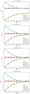 |
Fig. 4. Same as the topmost panel of Fig. 3 but for the γ specified in each panel’s title. |
| In the text | |
Current usage metrics show cumulative count of Article Views (full-text article views including HTML views, PDF and ePub downloads, according to the available data) and Abstracts Views on Vision4Press platform.
Data correspond to usage on the plateform after 2015. The current usage metrics is available 48-96 hours after online publication and is updated daily on week days.
Initial download of the metrics may take a while.