| Issue |
A&A
Volume 694, February 2025
|
|
|---|---|---|
| Article Number | A51 | |
| Number of page(s) | 17 | |
| Section | Stellar structure and evolution | |
| DOI | https://doi.org/10.1051/0004-6361/202451993 | |
| Published online | 31 January 2025 | |
Direct non-adiabatic modelling of gravito-inertial and Rossby tidally excited oscillations with the traditional approximation
STAR Institute, University of Liège, 19C Allèe du 6 Août, B-4000 Liège, Belgium
⋆ Corresponding author; This email address is being protected from spambots. You need JavaScript enabled to view it.
Received:
26
August
2024
Accepted:
18
November
2024
Abstract
Context. In recent years, the first detections of tidally excited stellar oscillations (TEOs) have been made in multiple star systems, offering new opportunities to study stellar physics and understand structural properties and stellar evolution. However, from a theoretical standpoint, numerous features in the observed oscillation spectrum cannot be explained, and current models cannot consistently treat the impact of stellar rotation on TEOs without using the Cowling approximation.
Aims. We aim to include the effect of the rotation in the modelling of TEOs and to study its consequences on the oscillation spectrum.
Methods. We developed a new methodology to include the Coriolis force in the modelling of TEOs through the traditional approximation but consistently treating the potential perturbation by iteratively solving the Poisson equation.
Results. By consistently including the Poisson equation, a new kind of mode coupling arises that we call ‘gravitational coupling’. Looking at the global oscillation spectrum, we find that the rotation greatly impacts the type of modes excited by the companion. In general, we find that the Rossby modes dominate the oscillation spectrum of TEOs.
Conclusions. It is particularly important to account for gravitational coupling at high spin parameters for the ℓ = 2, m = 2, and m = 0 oscillation modes. By assuming the modes are uncoupled, a simple and consistent treatment of the Poisson equation is possible. Including the effect of rotation in binary oscillation codes is necessary in order to accurately account for the impact of dynamical tides on the orbital evolution of binaries and planetary systems.
Key words: celestial mechanics / binaries : close / binaries: general / stars: interiors / stars: oscillations
© The Authors 2025
 Open Access article, published by EDP Sciences, under the terms of the Creative Commons Attribution License (https://creativecommons.org/licenses/by/4.0), which permits unrestricted use, distribution, and reproduction in any medium, provided the original work is properly cited.
This article is published in open access under the Subscribe to Open model. This email address is being protected from spambots. You need JavaScript enabled to view it. to support open access publication.
1. Introduction
In recent years, detections of tidally excited stellar oscillations (TEOs) in multiple star systems have opened new opportunities to study stellar physics and understand stellar structural properties. TEOs have been observed across all types of classical pulsators, and particularly in low- and intermediate-mass binary stars located in the classical pulsator instability strips (Li et al. 2024).
From a theoretical perspective, in binary systems, oscillations can be excited by periodic forcing from the companion star through tidal interactions, which act similarly to a forced oscillator. Tidal forces can induce two primary effects: large-scale mass redistribution due to a global hydrostatic adjustment (i.e. equilibrium tides) and the excitation of internal oscillation waves (i.e. dynamical tides Zahn 1970, 1975). The present study focuses on the latter. The periodic perturbation from a companion can excite a broad spectrum of low-frequency stellar oscillations, including gravity waves, inertial waves, and Rossby waves. However, for standing waves to be excited, the perturbation frequency must be in tune with a free oscillation frequency of the star, producing a resonance. Non-linear mode excitation, where a single mode excites multiple daughter modes, may also occur (Weinberg et al. 2012; Guo 2020; Guo et al. 2022), as can the excitation of low-frequency travelling waves (Burkart et al. 2012; Bowman et al. 2019; Ratnasingam et al. 2019). Here, we focus on the case where the perturbation from the companion linearly excites a single standing wave.
Following the detection of TEOs, rapid progress was made in theoretical modelling methods to understand their behaviour. There have been two main approaches to modelling TEOs: direct modelling (Smeyers et al. 1998; Willems et al. 2003; Burkart et al. 2012; Valsecchi et al. 2013; Sun et al. 2023) and modal decomposition (Zahn 1970, 1975; Burkart et al. 2012; Fuller & Lai 2012; Fuller 2017). In the direct modelling approach, the properties of TEOs are obtained by modifying a stellar oscillation code to include the periodic perturbation from a companion. Two notable oscillation codes developed with this methodology are CAFein (Valsecchi et al. 2013) and gyre_tides (Sun et al. 2023), both of which account for non-adiabatic effects on the oscillation modes. In the modal decomposition approach first introduced by Zahn (1970, 1975), the perturbation from the companion is decomposed into a combination of free oscillation eigenfunctions with different weights. This methodology relies on the adiabatic assumption, and its validity becomes uncertain when considering non-adiabatic oscillation modes, leading to discrepancies in the upper layers of stars (see e.g. Sun et al. 2023).
A key advantage of the modal decomposition method is the possibility to include the effects of rotation via the traditional approximation (Fuller 2017). In contrast, incorporating rotational effects in direct modelling is less straightforward. Classical oscillation codes often rely on the traditional approximation coupled with the Cowling approximation (Cowling 1941; Townsend 2005), which neglects potential perturbation in the differential equation system and excludes the Poisson equation from the system to be solved. For dynamical tides, the potential perturbation is crucial, as the orbital migration due to the excitation of oscillation modes in the star is proportional to this perturbation (Smeyers et al. 1998; Willems et al. 2003; Valsecchi et al. 2013; Sun et al. 2023). When following the approach of Smeyers et al. (1998), Willems et al. (2003), Valsecchi et al. (2013), Sun et al. (2023), the potential perturbations have to be treated consistently, necessitating the simultaneous solution of the Poisson equation and the system of differential equations. In Witte & Savonije (1999a,b, 2001), Savonije & Witte (2002), Savonije (2005), an equivalent formalism is presented that only requires the density perturbation to compute the dynamical tides, meaning that in this case the Cowling approximation can be used.
In this article, we developed a new modelling methodology to include the effect of rotation when computing tidally excited oscillations using the direct modelling methodology following the approach of Smeyers et al. (1998), Willems et al. (2003), Valsecchi et al. (2013), Sun et al. (2023). In doing so, we avoid the Cowling approximation, which is expected to be valid primarily for oscillation modes with high radial or spherical orders (Unno et al. 1989). Our starting point is the non-adiabatic oscillation code MAD (Dupret 2001; Dupret et al. 2002), which has already been modified to compute inertial and Rossby waves under the traditional approximation and the Cowling approximation (Bouabid et al. 2013). We further adapt this code to compute tidally excited oscillations, iteratively solving the Poisson equation to consistently include the effects of rotation.
In Sect. 2, we present the MAD code and describe the implementation of gravito-inertial wave computation via the traditional approximation, along with the modifications necessary to account for the effects of rotation on the Poisson equation. Sect. 3 focuses on our implementation of the rotation effects, with particular emphasis on our new mode coupling induced by modifications to the Poisson equation. In Sect. 4, we then study the global oscillation spectrum of binary stars, including the effect of rotation, and look at the impact of different properties of the system. Finally, in Sect. 5, we discuss the results obtained and the links between the approach of Smeyers et al. (1998), Willems et al. (2003), Valsecchi et al. (2013), Sun et al. (2023) used in this article and the approach of Witte & Savonije (1999a,b, 2001), Savonije & Witte (2002), Savonije (2005). Finally, we present our conclusions in Sect. 6.
2. Adapting our non-adiabatic free oscillation code (MAD) to compute dynamical tides
2.1. Non-adiabatic oscillations
In this article, we use our non-adiabatic oscillation code MAD (Dupret 2001; Dupret et al. 2002). This code has already been improved to include the effects of rotation (Bouabid et al. 2013), neglecting the centrifugal force and including the Coriolis force through the traditional approximation. In this approximation, the radial component of the Coriolis force and the effect of the radial displacement in the horizontal component of the Coriolis force are both neglected (Unno et al. 1989). This approximation is valid in the domain of low-frequency non-radial oscillations (when the frequency is smaller than the local Brunt-Vaisala frequency), where horizontal motion predominates. With this formalism, we are able to compute the properties of gravito-inertial and Rossby waves. However, it should be noted that the inclusion of the Coriolis force through the traditional approximation leads to misleading results for stars with large convective envelopes (Ogilvie & Lin 2004, 2007). In the present article, we focus on classical pulsators with thin convective envelopes or no convective envelope, such as γ Doradus and SPB stars.
To describe the formalism used for modelling free oscillations, we work in a spherical coordinate system (r, θ, ϕ) with the orthogonal basis (er, eθ, eϕ). In practice, to obtain the set of differential equations to solve, one must perturb the stellar structure equations (Unno et al. 1989).
The formalism of the equations used in MAD can be found in Appendix A. In MAD, we have a specific treatment of the stellar atmosphere, with its basic formalism detailed in Dupret (2001), Dupret et al. (2002). We note that MAD also includes the time-dependent convection model of Grigahcène et al. (2005), if needed. In this section, we reiterate the dynamic part of the basic set of differential equations classically employed to model the oscillations of non-rotating single stars and then the modified equations to include the effect of rotation through the traditional approximation. For non-rotating stars, the perturbation of each quantity can be decomposed on a spherical harmonics basis with
 (1)
(1)
With this decomposition, all the equations can be separated and solved independently for each ℓ, m, and k to obtain the perturbation of each quantity. The perturbation of an element can either be described by the Lagrangian perturbation formalism, which follows a fixed mass element, or the Eulerian perturbation formalism, which follows a fixed position in space. In this article, we denote the Lagrangian perturbation of an element X with δX and the Eulerian perturbation of this element with X′. The equations governing the dynamics of oscillations are the radial motion equation, the continuity equation, and the Poisson equation, which are respectively written as:
 (2)
(2)
 (3)
(3)
and
 (4)
(4)
In these equations, σ is the angular frequency of the oscillation mode considered (noted σℓ, km in Eq. (1)), ξr is the radial component of the displacement, ψ′ is the Eulerian perturbation of the gravitational potential, g is the effective gravity, ρ is the density, and P is the pressure.
When considering rotation in single stars using the traditional approximation, all quantities must be expanded into an infinite sum of Hough functions to preserve the separability of the equations of motion. In this work, we assume uniform rotation and adopt a coordinate system co-rotating with the star. It should be noted that the traditional approximation can also be extended to include differential rotation (Ogilvie & Lin 2004; Mathis 2009). In the case of solid body rotation, each quantity can now be written in the form:
 (5)
(5)
where Θℓ, νm(μ) are the Hough functions. These functions depend on the spin parameter ν, defined as:
 (6)
(6)
where Ω⋆ is the angular rotation rate of the star. With this formalism, the radial motion equation remains unchanged and is written as in Eq. (2). The continuity equation is modified to include the effect of the change of basis and is now written as
 (7)
(7)
where  are the eigenvalues of the Laplace tidal equation. The main drawback of decomposing the different quantities on the Hough basis is that the Poisson equation cannot be separated. This means that the equation cannot be solved independently for each oscillation mode projected onto the Hough basis; the oscillation modes are coupled in this basis for this equation. The direct consequence is that the Poisson equation can only be written in its general form:
 (8)
(8)
where Δ is the Laplace operator. In the traditional approximation, the perturbation of the gravitational potential and its derivatives are typically neglected in all equations of the system to avoid solving the Poisson equation. This additional simplification, known as the Cowling approximation, is frequently employed along with the traditional approximation when modelling non-adiabatic oscillation modes (Witte & Savonije 1999a,b, 2001; Savonije & Witte 2002; Townsend 2005; Savonije 2005; Bouabid et al. 2013). However, in the context of binary stars and dynamical tides, the accurate treatment of potential perturbations is essential for studying the influence of dynamical tides on the orbital evolution of the system when following the approach of Smeyers et al. (1998), Willems & Claret (2002), Willems et al. (2003). An alternative formalism, introduced by Witte & Savonije (1999a,b, 2001), Savonije & Witte (2002), Savonije (2005), requires only the density perturbation to analyse the effects of dynamical tides on the orbital evolution of binary systems. In Sect. 5, we discuss the key discrepancies between this approach and our methodology, as well as the methodology of Smeyers et al. (1998), Willems & Claret (2002), Willems et al. (2003). We explored the validity of the Cowling approximation in Appendix B and find that this approximation is not certain for low-radial-order modes.
In the present work, we do not use the Cowling approximation; we adopt the approach of Smeyers et al. (1998), Willems & Claret (2002), Willems et al. (2003), consistently solving the Poisson equation through the iterative process described in Sects. 2.3 and 2.4.
2.2. Tidally excited oscillations for non-rotating stars
In the previous section, we describe the methodology used in MAD to compute the free oscillations of single stars. In this section, we present the adaptations required in MAD to compute the oscillation modes (without stellar rotation) excited by the periodic tidal perturbation from a nearby star. The modifications can be divided into two parts: the inclusion of the perturbation from the companion, as presented in Sect. 2.2.1, and the modifications of the algorithm used to solve the system, as presented in Sect. 2.2.2.
2.2.1. Inclusion of the perturbation from the companion
For non-rotating stars, the dynamical part of the system of equations to solve is given in Eqs. (2) and (3). The impact of the companion appears by adding the gradient of the potential generated by the companion in the motion equation, which gives
 (9)
(9)
and
 (10)
(10)
where ψ2 is the potential from the secondary evaluated at each layer of the primary and projected onto a spherical harmonics basis. By adding the presence of the companion, the Poisson equation remains unmodified, as ψ2 is a solution of the Laplace equation. The gravitational potential from the companion is classically obtained using the perturbative approach, where it is implicitly assumed that stellar deformations are small departures from the spherical symmetry compared to the radius of the star. In this work, and as is customary when modelling tidally forced oscillations, the secondary is approximated by a point mass (Witte & Savonije 1999a,b, 2001; Savonije & Witte 2002; Townsend 2005; Savonije 2005). Within this approximation and in the perturbative framework, the tidal perturbing potential from the companion can be decomposed with a Fourier series and on the coordinate frame centred on the primary with
 (11)
(11)
where ℳ is the mean anomaly (ℳ = Ωorbt), and  is a normalisation coefficient defined as
 (12)
(12)
where Ωorb is the orbital rotation rate.  are the Hansen coefficients, which are defined as
 (13)
(13)
where v is the true anomaly of the system, e is its orbital eccentricity, a is its semi-major axis, and rsep is the instantaneous separation of the binary, which is defined for a given true anomaly as
 (14)
(14)
The coefficients  correspond to cℓ, m, k from Smeyers et al. (1998), Willems et al. (2003, 2010), Valsecchi et al. (2013). In the case of circular orbits we verified our numerical computation of
  with the values given in Willems et al. (2010). For a given oscillation mode, the radial component of the tidal perturbing potential is therefore given by
 (15)
(15)
which is the expression of the potential to insert in Eqs. (9) and (10). Furthermore, for tidally excited oscillations, the time-dependent part of the entire system of differential equations is decomposed into a Fourier series, as the perturbation from the companion is periodic.
In the case of non-rotating stars, Sun et al. (2023) pointed out that all the modifications presented in this section can be achieved by only modifying the surface boundary condition of the Poisson equation and solving the other equations using ψ′+ψ2 as the unknown related to the potential. Mathematically, the surface boundary condition of the Poisson equation has to be modified to
 (16)
(16)
This equation is obtained by adding ∂ψ2/∂r + ψ2(ℓ + 1)/r onto each side of the Poisson equation surface boundary condition (Eq. (C.11)); for more details about this boundary condition see Appendix C. By modifying either the surface boundary condition of the Poisson equation or the entire system of differential equations, the system to solve becomes inhomogeneous. Consequently, the algorithm for solving the system of equations must be modified, as presented in the following section.
2.2.2. Modifications of the algorithm
In the case of free oscillations, the system of equations to be solved is presented in the previous section. In practice, we express these equations in a matrix representation, which allows us to write the system of equations as
 (17)
(17)
where A and B are complex square-band matrices. The radial discretisation of the equations is achieved using staggered grids following the approach of Castor (1971); ten thousands points were used on each grid for the computations made in this article. In MAD, the eigenvectors x and eigenvalues σ are obtained using a generalised inverse-iteration algorithm. More details about the algorithm employed to solve the system, the matrix representation of the problem, and its discretisation can be found in Dupret (2001).
In the case of dynamical tides, since the perturbation from the companion is periodic and the system is developed in a Fourier series, the forcing frequencies σ are determined by the orbital properties of the system and stellar rotation. Instead of solving the system of equations for a single frequency, a dependency on k appears, and the system must be solved independently for different values of k, both positive and negative. Mathematically, the forcing frequencies are expressed in the corotating frame for a given orbital and stellar rotation rate, as
 (18)
(18)
It should be noted that in the present article, we adopt the sign convention for k of Valsecchi et al. (2013), whereas Sun et al. (2023) adopted the opposite sign convention. We also adopt the convention that σm, k should remain positive. If a negative frequency is obtained, the same oscillation mode can be studied by considering an opposite of m and k. With our sign conventions, km < 0 corresponds to prograde waves and km > 0 to retrograde waves in the inertial frame. Prograde waves in the inertial frame have larger amplitudes in general because their Hansen coefficients are larger. Furthermore, m > 0 corresponds to retrograde waves and m < 0 to prograde waves in the corotating frame. In this paper, when not specified, ‘prograge or retrograde’ means prograde or retrograde in the corotating frame, which is important in terms of mode physics.
The only ‘unknowns’ of the problem are the eigenfunctions of each oscillation mode. Moreover, as shown in Sect. 2.2.1, the inclusion of the perturbation from the companion transforms the system to be solved into an inhomogeneous set of differential equations. The new system to be solved can be written as
 (19)
(19)
where C is a complex vector containing the inhomogeneous part of the system of differential equations. To solve Eq. (19) we used the LU factorisation already implemented in MAD but without the inverse iterative algorithm, as the frequency is now an input parameter given by Eq. (18) and is no longer the free oscillation frequency.
2.3. Including the effects of rotation: The uncoupled approximation
When including the effects of rotation, the modifications made to the solving algorithm presented in Sect. 2.2.2 remain valid, as the system of equations remains inhomogeneous. However, modifying the surface boundary condition of the Poisson equation to include the perturbation from the companion is not feasible, as the Hough functions do not allow separation of the Poisson equation. In this section, we present the new methodology we developed to include the Coriolis force through the traditional approximation, using what we refer to as the ‘uncoupled approximation’ to separate the Poisson equation.
In the framework of the traditional approximation, as shown in Sect. 2.1, we require all the equations and quantities to be projected and decomposed on the Hough basis to solve the system of differential equations presented in Eqs. (2), (7), and (8). In the case of the Poisson equation, as written in Eq. (8) the projection on the Hough basis can be obtained using
 (20)
(20)
where ⟨…|…⟩ denotes the scalar product on a sphere. The right-hand side of Eq. (20) is not the major problem here, as it can be separated by decomposing ρ′ on the Hough basis. The problem of separability comes from the left-hand side of the equation. By decomposing ψ′ on the Hough basis, it can be rewritten as
 (21)
(21)
which can be rewritten to emphasise the dominant term of decomposition as follows:
 (22)
(22)
If the system of equations is uncoupled and one mode dominates the decomposition, then the last term of the previous equation can be neglected; we call this assumption the ‘uncoupled approximation’. This approximation is valid when there is one dominant mode in the decomposition, which typically occurs at low spin parameters or near resonance, as we show below. By using this approximation, the Poisson equation can be rewritten as
 (23)
(23)
where
 (24)
(24)
is the coupling term as given by Fuller (2017) in the case of modal decomposition. To estimate zℓm, Fuller (2017) uses an integral representation of the scalar product. However, in our case we are using the properties of the Hough functions to obtain this parameter; these properties are described in Appendix D. To maintain consistency with our stellar oscillation code, we introduce a modified spherical order  , such as
  . On the Hough basis and under the uncoupled approximation, the potential close to the centre of the star is proportional to
  , while close to the surface and outside of the star it is proportional to
  . The surface boundary conditions of the Poisson equation are also modified by the inclusion of the Coriolis force. Those conditions are obtained by imposing the continuity of the potential perturbation and its derivative between the inner solution of the Poisson equation and the outer solution of the Laplace equation. Using the same formalism as in Eq. (23) the boundary condition of the Poisson equation can be expressed as
 (25)
(25)
With the uncoupled approximation, Eq. (23) can be solved with Eqs. (2) and (7) on the Hough basis, as is traditionally done when computing tidally excited oscillations without including the effect of rotation. The main uncertainty of this approximation is the degree of validity of the uncoupled approximation; in Sect. 2.4 we present a new modelling method that fully includes the mode coupling.
2.4. Iterative solving of the Poisson equation: The coupled solution
The novelty of our new methodology is that we treat the potential perturbation as an inhomogeneous term in Eqs. (2) and (3), thereby separating the solving of the Poisson equation from that of the main system of differential equations. We then iteratively solve the system of differential equations for several Hough oscillation modes before combining them to solve the coupled Poisson equation and obtain the potential perturbations. As the coupling of the oscillations is arising from the non-separability of the Poisson equation, we call this mode coupling ‘gravitational coupling’.
In the case of the coupled oscillations, the Poisson equation, as written in Eq. (22) can be expanded using the projections presented in Eq. (D.1) of Appendix D, and can be expressed as
 (26)
(26)
where we define
 (27)
(27)
With this formulation, solving the Poisson equation for a given oscillation mode requires the potential perturbation from modes with the same ℓ parity and same m. In theory, this equation should be solved simultaneously for those few oscillation modes. In our modelling method, we have chosen to iteratively solve the system of equations for each oscillation mode, coupling the oscillations through the Poisson equation at each iteration step. It is well known that the projections of the potential on spherical harmonics are solution of an integral equation. We note that a similar result is found for the projections on the Hough basis. The potential given by the following integral relation is the solution of the Poisson equation (Eq. (26)):
 (28)
(28)
Our iterative process uses this method to solve the coupled Poisson equation. The iterative process is designed as follows:
-
We independently solve the system of differential equations for all the oscillation modes from ℓ′=m to ℓ′=L with the same parity as m using our uncoupled approximation. This provides us with an initial estimation of
 , δρ, and ξr.
 -
For all the oscillation modes, we couple our oscillations by computing
 and independently solving the Poisson equation with Eq. (28) to obtain
  .
. -
We then solve the system of differential equations again, excluding the Poisson equation and treating the previously obtained potential perturbation as an independent term in the motion and continuity equations.
-
If the code has not converged, we go back to the second step with the newly obtained δρ and ξr.
2.5. Verifications of the methodology
The numerical implementation of our method was made step by step to ensure the numerical stability and correctness of each portion of the code. Initially, we used a version of MAD that computed free gravito-inertial modes using the traditional approximation. We then implemented tidal forcing by modifying the surface boundary condition of the Poisson equation, as presented in Sect. 2.2.1. We then implemented the tidal forcing through the modifications of the whole system of differential equations, as described in Sect. 2.2.1, decoupled the Poisson equation, and solved it independently. We verified that both versions of the tidal forcing were giving the same results and eigenfunctions for a few oscillation modes for a given stellar model. We then proceeded to modify MAD to include the effect of rotation through the full iterative scheme described in Sect. 2.4.
For the presentation of the results in this article, we define the following dimensionless variables:
 (29)
(29)
where M is the mass of the studied star and R is its radius. To verify the validity of our new tidal oscillation method in a non-rotating case, we wanted to compare it with two existing tidal oscillation codes: CAFein (Valsecchi et al. 2013) and gyre_tides (Sun et al. 2023). However, our version of MAD is currently optimised to work with our stellar evolution code, the Code Liégeois d’Evolution Stellaire (CLES, Scuflaire et al. 2008), which guarantees models with high radial precision to accurately compute stellar oscillations. Consequently, we cannot use models from MESA, as used in CAFein and gyre_tides. This limitation means direct comparisons of oscillation results are not feasible due to differences in stellar structures. A comprehensive comparison of all three oscillation codes would require careful consideration and could be the focus of future research.
To mitigate this problem, we decided to directly compare our findings with published results, in particular all the results given in Valsecchi et al. (2013). We computed a stellar model equivalent to the model of the SPB star presented in Valsecchi et al. (2013) with CLES, ensuring it matched the characteristics of their twin binary system. Our stellar model has a mass of 5.0 M⊙, an initial metallicity of 0.18, and we evolve our star until the central hydrogen reaches XC = 0.5, at which point we verify with OSC that the free oscillation of the g-modes is close to that found by Valsecchi et al. (2013). For the stellar modelling, we used the AGSS09 abundances (Asplund et al. 2009), the FreeEOS equation of state (Irwin 2012), the OPAL opacities (Iglesias & Rogers 1996), the T(τ) relation from Model-C of Vernazza et al. (1981) for the atmosphere, the mixing length theory of convection implemented as in Cox & Giuli (1968), and the nuclear reaction rates of Adelberger et al. (2011). We then used the same setup for the binary as Valsecchi et al. (2013); namely we studied the quadrupolar tidally induced oscillation, with m = 0 and k = 1, for a twin binary system with an eccentricity of 0.4. We then reproduced different figures from Valsecchi et al. (2013); in particular we look at the surface radial displacement for our twin binary around two resonances (Fig. 5 from Valsecchi et al. 2013). Fig. 1 illustrates this displacement as a function of the dimensionless frequency σT ( ).
).
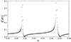 |
Fig. 1. Surface radial displacement of the mode ℓ = 2, m = 0, and k = 1 for the twin binary system composed of 5.0 M⊙ SPB stars with an eccentricity of 0.4. This figure is a reproduction of Fig. 5 of Valsecchi et al. (2013). |
For the same binary system, we also verified the eigenfunction of the tidally excited oscillations, as illustrated in Fig. 2.
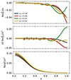 |
Fig. 2. Eigenfunctions of the mode ℓ = 2, m = 0, and k = 1 for the twin binary system composed of 5.0 M⊙ SPB stars with an eccentricity of 0.4. The top panel correspond to the radial displacement, the middle to panel is the horizontal displacement and the bottom panel is the potential perturbation. The eigenfunction can be directly compared to Fig. 7 of Valsecchi et al. (2013). |
3. Exploration of gravitational coupling
In this section, we explore the gravitational coupling of oscillation modes due to rotation. As it is well known that ℓ = 2 tides are dominating, we only consider modes with even values of ℓ.
3.1. Generalities about gravitational coupling due to rotation
The gravitational coupling between oscillations modes is defined by the cℓ′,ℓ,km coefficients, which are highly dependent on the value of the spin parameter. According to Eq. (26), the coupling between two oscillation modes is particularly dependent on the product cℓ, ℓ′mcℓ″, ℓ′m, and its value compared to (cℓ, ℓm)2 (the coefficient linked to the uncoupled term). If (cℓ, ℓm)2 ≫ cℓ, ℓ′mcℓ″, ℓ′m then the coupling is weak and the solution is dominated by the uncoupled term and the uncoupled approximation is valid. On the contrary, if (cℓ, ℓm)2 ∼ cℓ, ℓ′mcℓ″, ℓ′m then the coupling starts to play a role and impacts the oscillation modes. The cℓ″, ℓ′m coefficients are model independent and are only affected by the values of ℓ, ℓ′,m, and the spin parameter ν. Therefore, it is possible to make a model-independent comparison of these coefficients as a function of the spin parameter. Fig. 3 shows the evolution of the ratio cℓ, ℓ′mcℓ″, ℓ′m/(cℓ, ℓm)2 in a case where we only consider the coupling between the ℓ = 2 and ℓ = 4 oscillation modes.
 |
Fig. 3. Ratio of the coupling coefficient for a coupling between the ℓ = 2 and ℓ = 4 oscillation modes as a function of the spin parameter and for different values of m. |
This figure directly shows in which regime of the spin parameter and for which oscillation modes the gravitational coupling has an effect. For all the oscillations modes, Fig. 3 indicates that below a spin parameter of ν < 1.2, the mode coupling does not impact the ℓ = 2 oscillation modes. For the prograde modes (m = −2), even at high spin parameters, the coupling remains low and the uncoupled approximation is valid. This result is expected given the significant discrepancy in terms of λ between the ℓ = 2 and ℓ = 4 prograde modes (see Fig. 34.3 of Unno et al. 1989; λ(ν) tends towards a small value for ℓ = 2, while it increases significantly with ν for ℓ = 4.). We still attempted to compute the coupling, but we found that not only is the coupling factor small, but the potential perturbation of the ℓ = 4 prograde mode is several orders of magnitude smaller than the quadrupolar mode, making the coupling effectively null.
For the m = 0 modes, we see that the coupling drastically increases after ν = 1.2 and is the strongest overall. We explore the quantitative impact of this strong coupling on the oscillation modes in Sect. 3.2. For the retrograde mode (m = 2), we see that the coupling starts to become significant when ν > 1.2, reaches a plateau around ν = 3, and then slowly decreases. The quantitative effect of this coupling on the oscillation modes is explored in Sect. 3.3.
Finally, by including the effect of rotation through the traditional approximation, a fourth type of oscillation mode appears: the Rossby modes, which are low-frequency ℓ = 2, m = 2 oscillation modes. The latitudinal index k of the l = 2, m = 2 Rossby modes according to the classification of Lee & Saio (1997) is k = −2 (which is not to be confused with the Fourier index k used in this paper). Following Saio et al. (2018), in order to propagate in radiative zones (λ > 0), Rossby modes must have spin parameters that are larger than ν > (m + |k|)(m + |k|−1)/m, which gives ν > 6 for the l = 2, m = 2 Rossby modes. Specifically, in Fig. 1 of Saio et al. (2018), we see that, for the l = 2, m = 2 Rossby modes, λ > 0 when ν > 6; and in their Fig. 7, we can see the geometry of those modes. Rossby modes have low λ, contrary to the classical retrograde gravito-inertial modes. Consequently, due to the significant difference in λ, the mode coupling is negligible between the Rossby modes and the classical retrograde modes. In this section, the coupling of oscillation modes was computed up to ℓ = 10 for the retrograde and m = 0 oscillation modes, neglecting higher-order modes and the coupling of the Rossby and prograde modes.
3.2. ℓ = 2, m = 0 oscillation modes
In this section, we explore the impact of the gravitational coupling on the surface properties of the ℓ = 2, m = 0 oscillations modes, focusing in particular on the surface imaginary part of the potential perturbation, as this quantity directly impacts the evolution of the orbital parameters of the system (Smeyers et al. 1998; Willems et al. 2003; Valsecchi et al. 2013; Sun et al. 2023). From the previous section, we know that the coupling is negligible below a spin parameter of ν = 1.2. In the present section, we focus on the cases where ν > 1.2. We used the same SPB stellar model as in Sect. 2.5, and looked at the same scenario: a twin binary system composed of two of those SPB stars with an orbital eccentricity of 0.4. Our first objective was to quantify the effect of mode coupling on unstable oscillation modes with different stellar rotation rates. Figure 4 illustrates the difference in the surface imaginary part of the potential perturbation between the uncoupled and coupled versions of our code for two values of the stellar rotation rate, and for the same gravito-inertial oscillation mode (n = 11).
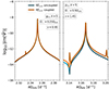 |
Fig. 4. Surface imaginary part of the potential perturbation for the ℓ = 2, m = 0, n = 11, k = 5 oscillation mode. The left panel corresponds to a case where the stellar rotation frequency is 0.25 Ωcrit = 1.15 d−1, while in the right panel the stellar rotation frequency is 0.5 Ωcrit = 2.29 d−1. The orange curves correspond to the results of the coupled oscillation code, while the blue curves correspond to the solution from the uncoupled oscillation code. The dark curves correspond to negative values of the potential perturbation while the lighter curves corresponds to positive values. |
From the left part of the figure, we observe that the coupling between oscillation modes, as expected, is low when ν < 1.2. However, even in this case, we can see small peaks in the imaginary part of the potential perturbation, which are associated with the ℓ = 4, m = 0 oscillation modes. These resonances impact the ℓ = 2 modes even if the coupling is low. As the spin parameter increases, we observe an overall difference across the entire spectrum; in the case presented here, there is a factor 2 difference between the solutions given by the uncoupled and coupled oscillation codes in the wings of the resonance. As expected, near the ℓ = 2 resonance, the two oscillation codes are equivalent, because one mode dominates. We can also see that with the increase in coupling, the effect of the ℓ = 4 resonances on the ℓ = 2 oscillations starts to become stronger. Finally, we can observe a change of sign on the imaginary part of the potential pertubation in the right panel of Fig. 4. This change of sign corresponds to a transition from a damping toward an excitation of an oscillation mode.
We then wanted to verify the impact of the coupling on stable oscillation modes, as the coupled oscillation code shows the greatest difference when no single oscillation mode dominates and for modes with large radial orders where the spin parameter is high. For the same binary system, we chose the stable oscillation with ℓ = 2, m = 0, n = 25, k = 5. Figure 5 illustrates the difference in the surface imaginary part of the potential perturbation around a stable oscillation mode for different values of stellar rotation.
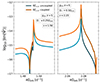 |
Fig. 5. Surface imaginary part of the potential perturbation for the ℓ = 2, m = 0, n = 25, k = 5 oscillation mode. The left panel corresponds to a case where the stellar rotation frequency is 0.25 Ωcrit = 1.15 d−1, while in the right panel the stellar rotation frequency is 0.5 Ωcrit = 2.29 d−1. The orange curves correspond to the results of the coupled oscillation code, while the blue curves correspond to the solution from the uncoupled oscillation code. The dark curves correspond to negative values of the while the lighter curves corresponds to positive values. |
For this mode, we already see a greater difference between the uncoupled and coupled oscillation codes. In this case, as the frequencies of the oscillation modes are smaller, the spin parameter is greater, making the coupling more significant for these oscillation modes. In the case of medium stellar rotation (Ω⋆ = 0.25 Ωcrit), the difference between the two codes is uniform, with about a factor of 2 difference. Here, we do not observe any impact from ℓ = 4 resonances, as in this regime of frequency the ℓ = 4, m = 0 oscillation modes have overly high radial orders. In the case of high rotation, the coupling of the oscillation uniformly increases the imaginary part of the potential perturbation by an order of magnitude. Importantly, at the resonance, the difference between the two oscillation codes also increases by an order of magnitude. This is explained by the retroactive effect of coupling when the spin parameter is significant. More specifically, the resonance of the ℓ = 2 mode significantly impacts the ℓ = 4 mode, which, due to the high coupling, can retroactively impact the ℓ = 2 modes.
3.3. Retrograde modes (ℓ = 2, m = 2)
In the case of the retrograde modes, from Fig. 3, we expected a weaker gravitational coupling than for the m = 0 modes. To verify the strength of coupling, with Fig. 6, we studied the model discrepancy as done in Sect. 3.2 for the n = 11 and n = 25 retrograde oscillation modes, when the stellar rotation frequency is 0.5 Ωcrit = 2.29 d−1.
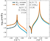 |
Fig. 6. Surface imaginary part of the potential perturbation for the ℓ = 2, m = 2, n = 25, k = −5 oscillation mode on the left, and for the ℓ = 2, m = 2, n = 11, k = −5 oscillation mode on the right. The orange curves correspond to the results of the coupled oscillation code, while the blue curves correspond to the solution from the uncoupled oscillation code. The dark curves correspond to negative values of the potential perturbation, while the lighter curves correspond to positive values. |
As expected, by comparing Figs. 4 (right panel), 5, and 6, we see that for the m = 2 oscillation modes, the mode coupling plays a less important role than for m = 0 oscillation modes. For stable modes at high spin parameters, we still see differences between the two modelling methods of about a factor of 5 (Fig. 6, left panel). For the unstable modes (Fig. 6, right panel), the discrepancies remain small.
4. Resonance spectra of fast-rotating stars
In this section, we model and study the global resonance spectra of binary stars, including the effect of rotation as described previously. In Sect. 4.1, we present the global scan of the oscillation spectrum done with our code for a twin system composed of two fast-rotating 3.5 M⊙ SPB stars. Then, in Sect. 4.2, we study the impact of rotation on the spectra of this system. Finally, in Sect. 4.3, we study the impact of different eccentricities on the spectra of the same binary system.
4.1. Global and local oscillation spectra
In this section, we create and analyse the resonance spectra of a binary system. For this study, we computed stellar models of an SPB star with a mass of 3.5 M⊙ with the same other ingredients as the stellar model described in Sect. 2.5. One key application of including rotation effects into our oscillation code is the ability to model tidally excited Rossby oscillation modes. We chose to use a different stellar model for this study because the previous model lay outside the instability strip for Rossby modes (Townsend 2005), whereas 3.5 M⊙ stars are inside this instability strip.
Efficiency is crucial for conducting a comprehensive scan of the oscillation spectrum, particularly when including modes with different k and m values, as well as systems with varying orbital properties. For all results presented here, we used the uncoupled version of our stellar oscillation code due to its faster execution time. With this version, we implemented a scan strategy that is independent of the system’s orbital parameters and k. The methodology takes advantage of the linearity of the solutions with respect to ψ2: a value of ψ2 proportional to xℓ is imposed during the execution of the oscillation code, effectively ignoring the contribution from the Hansen coefficients, and allowing for spectrum scanning relative to the corotation frequencies for each m value and a specified rotation frequency. The spectrum is then computed for each scan by scaling the solutions with the actual ψ2 value, as given in Eq. (15), across all considered k values and desired orbital parameters. For quadrupolar modes, this approach requires four separate scans of the oscillation spectrum (one for each m, with the fourth for Rossby modes), with a subsequent reconstruction of all oscillations. This strategy significantly reduces computation time by avoiding the need for hundreds of individual scans. Moreover, this methodology works independently of the system’s orbital parameters, allowing heavy computations to be executed autonomously. This methodology is particularly advantageous as it allows the inclusion of detailed dynamical tides into orbital evolution codes. To ensure coherence in the amplitude of the studied oscillation modes, we maintained a constant density of corotation period points in our scans, focusing only on regions near resonances identified with the free oscillations code.
Figure 7 illustrates the amplitude scan of various oscillation modes for a twin binary system composed of 3.5 M⊙ stars, with a stellar rotation of 0.5Ωcrit and an orbital eccentricity of e = 0.4. Given the density of the spectrum, we chose to only illustrate the dominant modes with an amplitude higher than the threshold of 10−10. In all such resonance spectra, we divided ψ′ by k. Indeed, one sees from Eq. (18) that the widths of the resonance lines in terms of Ωorb are proportional to k−1. The impact of crossing a resonance on the orbital parameters of a system is proportional to the integral of the imaginary part of the potential taken over the width of the resonance. Therefore, by dividing ψ′ by k, we account for the effect of the widths of the resonance lines on the orbital evolution of the system.
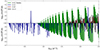 |
Fig. 7. Scan of the surface imaginary part of the potential perturbation as a function of the orbital rotation rate. The system studied is a twin binary system composed of 3.5 M⊙ stars with a stellar rotation frequency of 0.5 Ωcrit = 1.89 d−1 and an orbital eccentricity of e = 0.4. The top panel corresponds to positive values of the potential perturbation while the lower panel corresponds to negative values. The amplitudes of all the oscillation modes have been divided by k to magnify their width. |
This figure shows the dominance regime of each type of oscillation mode across different orbital separations. At lower orbital rotation rates (Ωorb < 1 d−1), the spectrum is dominated by retrograde oscillation modes (m = 2). As the orbital rotation rate increases, Rossby modes, in green, begin to dominate the spectrum, although retrograde modes still exhibit high-amplitude resonances in this regime. Generally, prograde and m = 0 oscillation modes do not significantly influence the spectrum in this scan. As illustrated in Fig. 7, the spectrum at high orbital rotation rate is very dense; Fig. 8 focuses on the part at higher orbital rotation rate, allowing us to identify the dominant oscillation modes and study the oscillation spectrum in more depth.
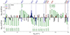 |
Fig. 8. Scan of the surface imaginary part of the potential perturbation for a limited portion of the orbital rotation rate. The system studied is a twin binary system composed of 3.5 M⊙ stars with a stellar rotation frequency of 0.5 Ωcrit = 1.89 d−1 and an orbital eccentricity of e = 0.4. The top panel corresponds to positive values of the potential perturbation, while the lower panel corresponds to negative values. In the upper part of the figure, the identification of the dominant oscillation can be found and is noted gn(k). The amplitudes of all the oscillation modes have been divided by k to magnify their width. |
The Rossby modes are m = 2 even modes with a dominating ℓ = 2 component able to produce high-amplitude resonances (see their geometry in the bottom-right panel of Fig. 2 in Saio et al. 2018). They all have spin parameters with values of greater than 6. For the stellar model and rotation considered, the Rossby modes of radial order 12 − 23 are unstable and they are stable outside of this interval. In Fig. 8, one can identify the unstable Rossby modes with positive Im( ), whereas stable modes have negative values. The spectrum reveals that Rossby modes form groups with varying radial orders but identical k. These separated groups come from the very low corotation frequencies of the Rossby modes. Imposing spin parameter values of greater than 6 and positive corotation frequencies gives:
 (30)
(30)
where k has to be negative so that these modes are prograde in the inertial frame and retrograde in the corotation frame. In practice, Rossby modes of lower radial order are found at the lower frequency limit, while higher-radial-order modes accumulate closer to the higher frequency limit. It is noteworthy that the density of Rossby modes increases with |k|, which can be seen in Fig. 7 for example.
The second major type of oscillation modes impacting the spectrum are the retrograde gravito-inertial oscillation modes (m = 2), which are shown in blue in Fig. 8, with a few large resonances, particularly at low k values. In the case of prograde modes, their propagation is constrained solely by their requirement to be prograde modes in the inertial frame:
 (31)
(31)
where k is negative for the same reason as for the Rossby modes. These resonances dominate the low-orbital-frequency part of the spectrum, where they have similar radial orders and different k. Indeed, a null frequency in the observer frame corresponds to a given value of the dimensionless mode frequency in the corotating frame equal to two times the dimensionless rotation frequency. For this rotation rate, no unstable retrograde modes are found, and the change in sign of the g11(−1) is due to the negative value of the Hansen coefficient when k = −1. As the modes are all stable, they all (except one) contribute in the same dissipative direction. In Figs. 7 and 8, we have added the modes retrograde in both the inertial and corotation frame (with k > 0). However, those modes do not play a significant role and only a few of them can be found at high orbital frequency in Fig. 7.
In the case of the prograde modes (m = −2), propagation is governed by the lower limit of the orbital frequency to ensure a positive corotation frequency:
 (32)
(32)
where k has to be positive. In practice, high-radial-order prograde modes accumulate close to this lower limit of the orbital frequency, while low-radial-order modes can be found at high orbital frequencies. In Fig. 8, no low-radial-order low-k prograde modes are found, as the required orbital frequency exceeds the orbital frequency leading to binary contact.
Finally, for the m = 0 oscillation modes, in the case of high rotation, low-order high-orbital-frequency oscillation modes require excessively high values of k to be visible. For this specific model at high rotation, we do not observe any unstable modes.
4.2. Impact of stellar rotation
In the previous section, we study the resonance spectrum for a fast-rotating star. In this section, we examine the impact of the stellar rotation rate on the oscillation spectrum of binary stars by decreasing the rotation. The results from this section can be anticipated based on the excitation criteria for modes discussed earlier; reducing the rotation changes the distribution of oscillation modes on the diagram. We used the same model as in the previous section, reduced the rotation frequency to 0.25 Ωcrit = 0.95 d−1, and performed the same global and local scans of the oscillation spectrum, as shown in Figs. 9 and 10, respectively.
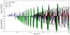 |
Fig. 9. Scan of the surface imaginary part of the potential perturbation as a function of the orbital rotation rate. The system studied is a twin binary system composed of 3.5 M⊙ stars with a stellar rotation frequency of 0.25 Ωcrit = 5.95 d−1 and an orbital eccentricity of e = 0.4. The top panel corresponds to positive values of the potential perturbation while the lower panel corresponds to negative values. The amplitudes of all the oscillation modes have been divided by k to magnify their width. |
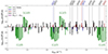 |
Fig. 10. Scan of the surface imaginary part of the potential perturbation for a limited portion of the orbital rotation rate. The system studied is a twin binary system composed of 3.5 M⊙ stars with a stellar rotation frequency of 0.25 Ωcrit = 5.95 d−1 and an orbital eccentricity of e = 0.4. The top panel corresponds to positive values of the potential perturbation, while the lower panel corresponds to negative values. In the upper part of the figure, the identification of the dominant oscillation can be found and is noted g radial order (k). In this figure, the amplitudes of all the oscillation modes have been divided by k to magnify their width. |
By comparing the spectra from this section with those of Sect. 4.1, several effects of the rotation can be directly observed. First, by decreasing the rotation, the retrograde gravito-inertial forces are significantly depleted, even at low orbital frequencies. This depletion is a direct consequence of the more than two times larger radial orders of these modes at a given orbital frequency. This is evident from the identification of the retrograde modes in Fig. 10; while in Sect. 4.1 the n = 11 can be found at high orbital frequency, here only the n = 23 − 24 are found in this regime.
On the other hand, the prograde modes have their lower orbital frequency limit shifted to lower frequencies, allowing modes with low radial orders and k to be found in the high-orbital-frequency regime. This results in an increase in the amplitude and importance of these modes at high orbital frequencies. At lower rotation frequencies, we also observe the appearance of unstable prograde modes, leading to both positive and negative Im , which could result in unpredictable effects from the dynamical tides.
Decreasing the rotation frequency also impacts the Rossby modes. Fewer unstable Rossby modes are found in the spectrum, and there is a decrease in the spread of Rossby modes, creating small areas with a high density of Rossby modes. Additionally, the decrease in rotation reduces the values of |k| at a given orbital frequency, which, with this eccentricity, increases the amplitude of the modes. From an orbital evolution standpoint, having well-localised areas with a high density of high-amplitude Rossby modes could significantly impact the system through dynamical tides.
Finally, for the m = 0 modes, lower rotation allows access to modes of lower radial order with higher amplitudes (due to the decrease of λ) at high orbital frequencies. In this regime, m = 0 modes can become as significant as the prograde oscillation modes.
4.3. Impact of eccentricity
The eccentricity of the binary system also impacts the scan of the oscillation spectrum by modifying the Hansen coefficients, and thereby influencing the significance of the orbital harmonics k. In Fig. 11, we illustrate the Hansen coefficient – as used in Eq. (15) – as a function of k for the ℓ = 2, m = 2 modes, and for different values of eccentricity.
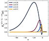 |
Fig. 11. Evolution of the Hansen coefficient as a function of k for the ℓ = 2, m = 2 modes and different eccentricities. |
Looking at the Hansen coefficients, we can see that higher eccentricity means that higher values of k play a key role. Consequently, in the oscillation spectrum of a binary system, higher eccentricity increases the amplitude of high k modes, potentially introducing new dominant oscillation modes and resulting in a denser spectrum. For the same binary system as in Sect. 4.1, Fig. 12 illustrates the global oscillation spectrum when the eccentricity is 0.7.
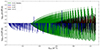 |
Fig. 12. Scan of the surface imaginary part of the potential perturbation as a function of the orbital rotation rate. The system studied is a twin binary system composed of 3.5 M⊙ stars with a stellar rotation frequency of 0.5 Ωcrit = 1.89 d−1 and an orbital eccentricity of e = 0.7. The top panel corresponds to positive values of the potential perturbation, while the lower panel corresponds to negative values. The amplitudes of all the oscillation modes have been divided by k to magnify their width. |
With increased eccentricity, oscillation modes with higher k values significantly impact the spectrum, making it denser. Specifically, Fig. 12 shows that the Rossby modes become more dense. For the retrograde modes, having higher k available does not significantly change the oscillation spectrum; it only becomes denser at low frequencies. This is because the accumulation of retrograde modes occurs below the limit given in Eq. (31), where higher k values correspond to lower orbital frequencies and thus higher orbital separations.
However, higher eccentricity significantly impacts the prograde and m = 0 modes. With higher k values, modes of low radial order can be reached at higher orbital frequencies. This effect is seen in Fig. 12, where, at lower orbital eccentricity, the prograde and m = 0 modes are almost non-existent, while at higher eccentricities, these modes become significant at high orbital frequencies. However, their amplitudes remain significantly lower than those of Rossby modes.
5. Discussion
In the above sections, we introduce and test a method to incorporate the effects of rotation into models of binary stellar oscillation without relying on the Cowling approximation. Although developed for binary systems, this formulation can also be implemented in classical non-adiabatic oscillation codes. To account for rotation while solving the Poisson equation, we developed two distinct approaches: the first considers only the dominant term for each oscillation mode, while the second fully accounts for a new type of coupling that we call gravitational coupling. We find that the gravitational coupling significantly affects the amplitude in the wings of resonances and for high spin parameters (ν > 1.5). Accounting for the gravitational mode coupling is important for accurately modelling the amplitudes of specific oscillation modes and comparing the models with observations.
By scanning the oscillation spectrum with the effects of rotation included, we identified patterns of mode accumulation and the dominant oscillation modes for various system configurations. Notably, Rossby modes emerge as dominant, occupying specific, dense regions of the spectrum. From the perspective of orbital evolution, computing these modes is critical, as these accumulation zones can significantly influence the orbital evolution of binary systems.
For prograde and m = 0 mode resonances, we expect their impact on orbital evolution to be weak due to their lower amplitudes and the opposing effects of stable and unstable modes. However, for Rossby modes, small regions in the orbital frequency domain could lead to rapid orbital evolution or even orbital trapping. Such trapping may also occur due to large, sparse resonances generated by retrograde oscillation modes. The rapid orbital evolution induced by Rossby modes could prevent the detection of binaries within these frequency domains.
According to Newton’s third law, the force exerted by the perturbed primary on the unperturbed secondary (proportional to the perturbation of the potential generated by the primary) is equal and opposite to the force exerted by the unperturbed secondary on the perturbed primary (proportional to the perturbation of the density of the primary). Exploiting this property, Witte & Savonije (1999a,b, 2001), Savonije & Witte (2002), Savonije (2005) developed a method for computing the orbital evolution that only requires the density perturbation, which allows the Cowling approximation to be used to study dynamical tides. This approach also consistently includes the effects of rotation without needing to solve the Poisson equation. In Witte & Savonije (1999a,b, 2001), Savonije & Witte (2002), a complete treatment of rotation with the Cowling approximation is adopted, while in Savonije (2005) the rotation is included with the traditional approximation still using the Cowling approximation.
A key difference between our approach and that of Savonije (2005) lies in the treatment of the Cowling approximation. In Appendix B, we assess the validity of the Cowling approximation and demonstrate that for low-radial-order modes, it becomes problematic, with both a shift in the frequency of the maxima and a discrepancy in relation to their amplitudes of about one order of magnitude. In these cases, solving the Poisson equation is necessary to obtain accurate amplitudes and frequencies for low-radial-order modes. In Appendix B, we only explore the validity of the Cowling approximation without including the effects of rotation; we expect the gravitational coupling to also have an impact on the validity of the Cowling approximation, and this could be the subject of another article.
In this work and in the literature (Witte & Savonije 1999a,b, 2001; Savonije & Witte 2002; Ogilvie & Lin 2004), multiple types of mode coupling –based on different physical processes– appear due to rotation. A first type of linear coupling comes from the fact that the Coriolis and centrifugal forces make the problem of non-radial oscillations non-separable. Under the traditional approximation, the terms responsible for this non-separability are neglected and the problem can be separated in terms of the Hough functions. However, this approximation is not valid, for example, for p-modes and in convective zones. In the present article, we investigate a second type of coupling that we call gravitational coupling. This coupling arises from the fact that the Hough functions are not eigenfunctions of the Laplace operator in the Poisson equation. The gravitational coupling allows for interaction between modes, like the classical mode coupling. In particular, quadrupolar modes are directly influenced by the potential perturbation of spherical modes of higher degrees, as shown in Fig. 4. When using the Cowling approximation, this gravitational coupling is neglected; however, we demonstrate that in the cases we study here, the Cowling approximation may not be fully valid. The validity of the Cowling approximation should also be impacted by the inclusion of gravitational coupling.
Finally, there is another effect that should not, by itself, be considered as a coupling. The tidal potential generated by the secondary is largely dominated by quadrupolar spherical harmonics (ℓ = 2). However, for high values of the spin parameter, the Hough functions of higher degrees have a non-negligible quadrupolar component. The associated modes are therefore tidally excited by the quadrupolar component of the tidal potential, but they remain ‘uncoupled’. Under the uncoupled approximation, the gravitational coupling is entirely neglected, even though a single forcing term may excite multiple modes; separability is assumed. This approach is similar to that used in Savonije (2005), where the Cowling approximation is also employed. In contrast, our coupled formalism takes into account the non-separability of the modes.
The modelling method presented here is not limited to binary systems; it can also be applied to planetary systems. Our approach for scanning the oscillation spectrum is independent of the companion’s properties and orbital parameters, and is well-suited for studying star–planet interactions. This method allows precise calculations of planetary evolution, including the effects of dynamical tides on the system’s orbital parameters.
Recently, Papaloizou & Savonije (2023, 2024) explored the excitation of Rossby modes by giant planets orbiting solar-type stars. The formalism used by these authors, which is closer to that of Ogilvie & Lin (2004, 2007), includes a full treatment of rotation, which is a necessary feature when studying tidally excited gravito-inertial or inertial oscillations in such systems. The primary limitation of our model lies in the applicability of the traditional approximation. While we focus on SPB stars in this article, the traditional approximation also remains valid for γ Doradus stars and more massive stars. Although most planets are found around low-mass stars, several γ Doradus stars host planets, making them promising targets for applying our methodology. In addition, a significant portion of binary systems exhibiting tidally excited oscillations are located within the γ Doradus instability strip, further emphasising their relevance as targets for our model. However, our method is not suitable for low-mass stars with extensive convective envelopes, such as those studied in Ogilvie & Lin (2004, 2007), Papaloizou & Savonije (2023, 2024).
6. Conclusion
In this work, we developed a new theoretical modelling procedure to include the effect of rotation on tidally excited oscillation modes through the traditional approximation, without using the Cowling approximation. We first present the basic formalism of tidally excited oscillations before introducing our new modelling procedure in Sect. 2. Then, in Sect. 3, we compare the two modelling methods we developed to identify the regime in which the uncoupled approximation is valid. In Sect. 4, we examine the impact of including rotation on the oscillation spectrum of binary systems before discussing the implications of our results in Sect. 5.
To include the effect of rotation on the oscillation modes, we developed two different methodologies. The first uses the uncoupled approximation, assuming no coupling between the oscillation modes in the Poisson equation. The second method iteratively solves the Poisson equation, including the effect of mode coupling without this assumption. We compared these two modelling methods for different types of oscillations. We determined that for prograde modes, mode coupling has no significant impact on the amplitude of the oscillation spectrum, even at high spin parameters. The same conclusion applies to Rossby modes. For the retrograde (l = 2, m = 2) oscillation modes, gravitational coupling mode coupling starts to affect the amplitude when the spin parameter exceeds 1.2. In the case studied here, involving an SPB star of 5.0 M⊙, we observed a factor of two increase in amplitude due to mode coupling. For the l = 2, m = 0 oscillation modes, the impact of coupling is greater, with differences of up to an order of magnitude in the amplitude of the oscillation waves within the same spin parameter regime as for the retrograde modes. Importantly, we find that the uncoupled version of the code is generally sufficient to model the amplitude of oscillations close to resonances, with most differences occurring out of resonance. The coupled version of the code is recommended for detailed modelling of the amplitudes of observed oscillation modes at high spin parameters, where accurately modelling the exact amplitude of the modes is essential.
Using the uncoupled version of our binary evolution code, we explored the total oscillation spectrum of a theoretical twin binary system composed of two 3.5 M⊙ SPB stars. At high stellar rotation rates, we observed that tidally excited Rossby modes completely dominate the oscillation spectrum at high orbital frequencies, while retrograde modes dominate at lower orbital frequencies. Due to their high amplitudes, high density and predictable positions in the resonance spectrum (see Eq. (30)), they are expected to have a significant impact on the orbital evolution of binary systems. In contrast, at high rotation rates, the prograde and m = 0 modes play a less significant role, exhibiting lower resonance amplitudes.
Exploring the oscillation spectrum at lower stellar rotation rates revealed a contrasting scenario: prograde and m = 0 modes now play a key role, with high-amplitude modes appearing at high orbital frequencies. Although Rossby modes still dominate overall, prograde and m = 0 modes exhibit comparable amplitudes, with less predictable positions. Decreasing the stellar rotation rate causes a significant reduction in the amplitudes of the retrograde modes. This phenomenon can be attributed to an increase in the radial order of the modes along with a decrease in rotation for a given orbital frequency. Furthermore, we investigated the impact of the orbital eccentricity on the oscillation spectrum and observed that increasing the eccentricity leads to a denser resonance spectrum. Notably, prograde and m = 0 modes can become significant even at high stellar rotation rates.
Given the significant impact of rotation on the oscillation spectrum of binary systems, a more comprehensive study is warranted to explore how dynamical tides affect the orbital evolution of these systems. The densely populated orbital frequency regions by high-amplitude Rossby modes suggest the potential occurrence of resonance locking or rapid orbital evolution at the accumulation points of these modes. Integrating our oscillation code with an orbital evolution code is essential and is planned for future research, allowing a detailed investigation into how rotation influences the orbital dynamics of binary systems via dynamical tides.
Acknowledgments
The authors thank the referee for their comments that helped to improve this paper. L.F was supported by the Fonds de la Recherche Scientifique F.R.S-FNRS as a Research Fellow.
References
- Adelberger, E. G., García, A., Robertson, R. G. H., et al. 2011, Rev. Mod. Phys., 83, 195 [Google Scholar]
- Asplund, M., Grevesse, N., Sauval, A. J., & Scott, P. 2009, ARA&A, 47, 481 [NASA ADS] [CrossRef] [Google Scholar]
- Bouabid, M. P., Dupret, M. A., Salmon, S., et al. 2013, MNRAS, 429, 2500 [Google Scholar]
- Bowman, D. M., Burssens, S., Pedersen, M. G., et al. 2019, Nat. Astron., 3, 760 [Google Scholar]
- Burkart, J., Quataert, E., Arras, P., & Weinberg, N. N. 2012, MNRAS, 421, 983 [NASA ADS] [CrossRef] [Google Scholar]
- Castor, J. I. 1971, ApJ, 166, 109 [NASA ADS] [CrossRef] [Google Scholar]
- Cowling, T. G. 1941, MNRAS, 101, 367 [NASA ADS] [Google Scholar]
- Cox, J. P., & Giuli, R. T. 1968, Principles of stellar structure [Google Scholar]
- Dupret, M. A. 2001, A&A, 366, 166 [NASA ADS] [CrossRef] [EDP Sciences] [Google Scholar]
- Dupret, M. A., De Ridder, J., Neuforge, C., Aerts, C., & Scuflaire, R. 2002, A&A, 385, 563 [NASA ADS] [CrossRef] [EDP Sciences] [Google Scholar]
- Fuller, J. 2017, MNRAS, 472, 1538 [Google Scholar]
- Fuller, J., & Lai, D. 2012, MNRAS, 420, 3126 [NASA ADS] [CrossRef] [Google Scholar]
- Grigahcène, A., Dupret, M. A., Gabriel, M., Garrido, R., & Scuflaire, R. 2005, A&A, 434, 1055 [NASA ADS] [CrossRef] [EDP Sciences] [Google Scholar]
- Guo, Z. 2020, ApJ, 896, 161 [NASA ADS] [CrossRef] [Google Scholar]
- Guo, Z., Ogilvie, G. I., Li, G., Townsend, R. H. D., & Sun, M. 2022, MNRAS, 517, 437 [NASA ADS] [CrossRef] [Google Scholar]
- Iglesias, C. A., & Rogers, F. J. 1996, ApJ, 464, 943 [NASA ADS] [CrossRef] [Google Scholar]
- Irwin, A. W. 2012, Astrophysics Source Code Library [record ascl:1211.002] [Google Scholar]
- Lee, U., & Saio, H. 1997, ApJ, 491, 839 [Google Scholar]
- Li, M.-Y., Qian, S.-B., Zhu, L.-Y., et al. 2024, ApJ, 962, 44 [NASA ADS] [CrossRef] [Google Scholar]
- Mathis, S. 2009, A&A, 506, 811 [CrossRef] [EDP Sciences] [Google Scholar]
- Ogilvie, G. I., & Lin, D. N. C. 2004, ApJ, 610, 477 [Google Scholar]
- Ogilvie, G. I., & Lin, D. N. C. 2007, ApJ, 661, 1180 [Google Scholar]
- Papaloizou, J. C. B., & Savonije, G. J. 2023, MNRAS, 520, 4376 [NASA ADS] [CrossRef] [Google Scholar]
- Papaloizou, J. C. B., & Savonije, G. J. 2024, MNRAS, 527, 4983 [Google Scholar]
- Ratnasingam, R. P., Edelmann, P. V. F., & Rogers, T. M. 2019, MNRAS, 482, 5500 [NASA ADS] [CrossRef] [Google Scholar]
- Saio, H., Kurtz, D. W., Murphy, S. J., Antoci, V. L., & Lee, U. 2018, MNRAS, 474, 2774 [Google Scholar]
- Savonije, G. J. 2005, A&A, 443, 557 [NASA ADS] [CrossRef] [EDP Sciences] [Google Scholar]
- Savonije, G. J., & Witte, M. G. 2002, A&A, 386, 211 [NASA ADS] [CrossRef] [EDP Sciences] [Google Scholar]
- Scuflaire, R., Théado, S., Montalbán, J., et al. 2008, Ap&SS, 316, 83 [Google Scholar]
- Smeyers, P., Willems, B., & Van Hoolst, T. 1998, A&A, 335, 622 [NASA ADS] [Google Scholar]
- Sun, M., Townsend, R. H. D., & Guo, Z. 2023, ApJ, 945, 43 [NASA ADS] [CrossRef] [Google Scholar]
- Takata, M. 2005, PASJ, 57, 375 [NASA ADS] [Google Scholar]
- Townsend, R. H. D. 2005, MNRAS, 360, 465 [NASA ADS] [CrossRef] [Google Scholar]
- Unno, W., Osaki, Y., Ando, H., Saio, H., & Shibahashi, H. 1989, Nonradial oscillations of stars [Google Scholar]
- Valsecchi, F., Farr, W. M., Willems, B., Rasio, F. A., & Kalogera, V. 2013, ApJ, 773, 39 [NASA ADS] [CrossRef] [Google Scholar]
- Vernazza, J. E., Avrett, E. H., & Loeser, R. 1981, ApJS, 45, 635 [Google Scholar]
- Weinberg, N. N., Arras, P., Quataert, E., & Burkart, J. 2012, ApJ, 751, 136 [NASA ADS] [CrossRef] [Google Scholar]
- Willems, B., & Claret, A. 2002, A&A, 382, 1009 [NASA ADS] [CrossRef] [EDP Sciences] [Google Scholar]
- Willems, B., van Hoolst, T., & Smeyers, P. 2003, A&A, 397, 973 [NASA ADS] [CrossRef] [EDP Sciences] [Google Scholar]
- Willems, B., Deloye, C. J., & Kalogera, V. 2010, ApJ, 713, 239 [NASA ADS] [CrossRef] [Google Scholar]
- Witte, M. G., & Savonije, G. J. 1999a, A&A, 341, 842 [NASA ADS] [Google Scholar]
- Witte, M. G., & Savonije, G. J. 1999b, A&A, 350, 129 [NASA ADS] [Google Scholar]
- Witte, M. G., & Savonije, G. J. 2001, A&A, 366, 840 [NASA ADS] [CrossRef] [EDP Sciences] [Google Scholar]
- Zahn, J. P. 1970, A&A, 4, 452 [NASA ADS] [Google Scholar]
- Zahn, J. P. 1975, A&A, 41, 329 [NASA ADS] [Google Scholar]
Appendix A: Formalism used in MAD
Including the effect of the rotation through the traditional approximation, the three components of the perturbed motion equation are written as
 (A.1)
(A.1)
 (A.2)
(A.2)
and,
 (A.3)
(A.3)
In the previous equations, σ is the frequency of the oscillation mode considered, ξr, ξθ and ξϕ are respectively the radial, latitudinal and longitudinal components of the displacement, ψ′ is the Eulerian perturbation of the potential, g is the effective gravity, ρ is the density, P is the pressure, and Ωrot is the stellar rotation rate. The solution of each quantity can be cast into the form of an infinite linear combination of functions given by
 (A.4)
(A.4)
where Θℓ, νm(μ) are the Hough functions, the eigenfunctions of the operator linked to Laplace tidal equation ℒν defined as
![Mathematical equation: $$ \begin{aligned} \mathcal{L} _\nu = \dfrac{d}{d\mu } \left[ \dfrac{1-\mu ^2}{1-\nu ^2 \mu ^2} \dfrac{d}{d\mu } \right]-\dfrac{1-\mu ^2}{1-\nu ^2 \mu ^2}\left[ \dfrac{m}{1-\mu ^2}+m\nu \dfrac{1+\nu ^2\mu ^2}{1-\nu ^2\mu ^2} \right], \end{aligned} $$](/articles/aa/full_html/2025/02/aa51993-24/aa51993-24-eq52.gif) (A.5)
(A.5)
where ν is defined as
 (A.6)
(A.6)
and μ = cos θ. Therefore, the horizontal displacement is given by
 (A.7)
(A.7)
In the continuity equations, the inclusion of the rotation through the traditional approximation modifies this equations as follows
 (A.8)
(A.8)
where  is the eigenvalue of the Hough function of the chosen oscillation mode. The equations of energy transport and conservation are unchanged by our the inclusion of the rotation through the perturbative approach. The system of equations solved in MAD for the stellar interior is already described in Dupret (2001), Dupret et al. (2002). The equations of the energy transport and conservation are respectively written as
 (A.9)
(A.9)
and, in the case of frozen convection,
 (A.10)
In the previous equations, T is the temperature of the layer considered, S is its entropy, L is its luminosity, ϵ is its energy production, LR is its radiative luminosity, LC is its convective luminosity, and κ is its oppacity.
Appendix B: Validity of the Cowling approximation
In this section, we examine the validity of the Cowling approximation, which neglects the perturbation of the gravitational potential in the continuity, mass conservation, and radial motion equations. Theoretically, this approximation is expected to be valid in the regime of high radial order and/or high spherical order oscillation modes (Unno et al. 1989). However, for low radial order and low spherical order oscillation modes, the validity of this approximation is not guaranteed. For dipolar modes, Takata (2005) already showed that this approximation is not always accurate.
The Cowling approximation, if not accurate, can induce both a shift in the frequencies of the oscillation modes and a difference in the amplitudes of the modes. Consequently, the validity of this approximation has to be verified with a global scan of the oscillation spectrum. While the formalism from in (Witte & Savonije 1999a,b, 2001; Savonije & Witte 2002; Savonije 2005) uses the integral of the imaginary part of the density pertubation over the volume of the star to study dynamical tides, our formalism uses the imaginary part of the gravitational perturbation, which can be obtained by integrating the imaginary part of the density perturbation over the radius of the star (see Eq. (28)). Therefore, the verification of the validity of Cowling can be done with a global scan of the oscillation spectrum, looking at the imaginary part of the potential perturbation, consistently obtained with our methodology or obtained a posteriori, with the density perturbation in the formalism with the Cowling approximation.
The validity of this approximation can already be tested without including rotational effects. For the 3.5 M⊙ SPB star model presented in Sect. 4, in Fig. B.1, we compare the surface Im(ψ′) obtained with and without the Cowling approximation around the m = 0, n = 11 and n = 5 oscillation modes.
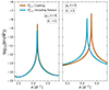 |
Fig. B.1. Imaginary part of ψ′ around the m = 0, n = 11 (on the left panel) and n = 5 (on the right panel) oscillation modes as a function of the forcing frequency. The orbital parameters of the system were we arbitrary chosen to be k = 8 and e = 0.4. |
We find almost no shift in frequency for the n = 11 oscillation mode due to the Cowling approximation. At the surface, we see an overestimation of approximately one order of magnitude in the imaginary part of the potential perturbation at the centre of the resonance line. Furthermore, we observe systematic difference in the amplitude of about one order of magnitude for low-radial oscillation modes, as seen for the n = 5 oscillation mode. In addition, for the n = 11 mode, we observe significant differences in the imaginary part of the potential perturbation, with an offset of the frequency of the maximum of about 0.030 d−1. For the m = 0 modes, this frequency shift is more important for lower radial order modes. This highlights the limitations of the Cowling approximation for modes with relatively low radial order. A more detailed investigation could be the subject of a future work, would explore the impact of the gravitational coupling on the limitations of the Cowling approximation.
Given these limitations, there is a clear difference between dynamical tide treatments based on potential perturbations (as used in this work) and those based on density perturbations, such as in the formalism by (Witte & Savonije 1999a,b, 2001; Savonije & Witte 2002; Savonije 2005). Although small frequency shifts and amplitude variations may have a minor impact on broad theoretical studies of the effect of dynamical tides on orbital evolution of binary system, they become important when attempting to model specific observed systems. This frequency shift can determine whether certain modes are theoretically resonating due to the companion forcing or not in tune and not observable.
Appendix C: Boundary condition of the Poisson equation
For the boundary condition of the Poisson equation we want to impose the continuity between the inner solution of the Poisson equation and outer solution of the Laplace equation. In the vacuum the solution of the Laplace equation tending towards 0 at infinity takes the form
 (C.1)
(C.1)
where ψℓm(R) is the component of the gravitational potential at the surface of stars. For what follows the dependency on ℓ and m is implicit. The first derivative with respect to the radial coordinate of the solution of the Laplace equation in the vacuum is
 (C.2)
(C.2)
The continuity of the Lagrangian perturbation of the gravitational potential and its derivative can be expressed as
 (C.3)
(C.3)
and,
 (C.4)
(C.4)
Those equations can be rewritten in the Eulerian formalism as
 (C.5)
(C.5)
and,
 (C.6)
(C.6)
The first derivative of the potentials are continuous, mathematically:
 (C.7)
(C.7)
Concerning the second derivative of the gravitational potential, we only have the continuity if the density is null, at the exterior of the star we have,
 (C.8)
(C.8)
and in the interior we have:
 (C.9)
(C.9)
By subtracting the last two equations, we obtain:
 (C.10)
By inserting this equality in Eq. (C.6), and using the expression of the radial derivative of the outer potential we obtain:
 (C.11)
which is the boundary condition for the Poisson equation used in the classical version of MAD (Sect. 2.1) and in Sect. 2.2.1. Later on, we chose to neglect the right hand side of Eq. (C.11) (as usually done, see Unno et al. (1989) ) as at the surface the density of the star is negligible. Finally, it can be shown with the same developments that with the uncoupled approximation, an equivalent expression of the boundary condition can be found and is given by Eq. (25).
Appendix D: Projections from and on the Hough basis
Mathematically, each Hough function can be defined as a combination of associated Legendre polynomials:
 (D.1)
(D.1)
where cℓ′,ℓ,km can be obtained by solving the Laplace tidal equation, we used a matrix representation of this equation as described in Unno et al. (1989) to obtain simultaneously the eigenvalue of each Hough function λ and the spectral decomposition on the associated Legendre polynomials.
Under the uncoupled approximation, these properties can be used to compute the coefficient zℓm as given by Eq. (24). In Eq. (24), we can decompose the Hough functions of the scalar product into associated Legendre polynomials using Eq. (D.1), then apply the Laplace operator as it separates the associated Legendre polynomials before applying the orthogonal properties of the associated Legendre polynomials. With these operations, zℓm is given by
 (D.2)
(D.2)
Through all this article, we approximate this sum by accounting for all the terms up to ℓ′ = 50, only the terms with the same parity as ℓ are non-zero.
All Figures
|
Fig. 1. Surface radial displacement of the mode ℓ = 2, m = 0, and k = 1 for the twin binary system composed of 5.0 M⊙ SPB stars with an eccentricity of 0.4. This figure is a reproduction of Fig. 5 of Valsecchi et al. (2013). |
| In the text | |
|
Fig. 2. Eigenfunctions of the mode ℓ = 2, m = 0, and k = 1 for the twin binary system composed of 5.0 M⊙ SPB stars with an eccentricity of 0.4. The top panel correspond to the radial displacement, the middle to panel is the horizontal displacement and the bottom panel is the potential perturbation. The eigenfunction can be directly compared to Fig. 7 of Valsecchi et al. (2013). |
| In the text | |
|
Fig. 3. Ratio of the coupling coefficient for a coupling between the ℓ = 2 and ℓ = 4 oscillation modes as a function of the spin parameter and for different values of m. |
| In the text | |
|
Fig. 4. Surface imaginary part of the potential perturbation for the ℓ = 2, m = 0, n = 11, k = 5 oscillation mode. The left panel corresponds to a case where the stellar rotation frequency is 0.25 Ωcrit = 1.15 d−1, while in the right panel the stellar rotation frequency is 0.5 Ωcrit = 2.29 d−1. The orange curves correspond to the results of the coupled oscillation code, while the blue curves correspond to the solution from the uncoupled oscillation code. The dark curves correspond to negative values of the potential perturbation while the lighter curves corresponds to positive values. |
| In the text | |
|
Fig. 5. Surface imaginary part of the potential perturbation for the ℓ = 2, m = 0, n = 25, k = 5 oscillation mode. The left panel corresponds to a case where the stellar rotation frequency is 0.25 Ωcrit = 1.15 d−1, while in the right panel the stellar rotation frequency is 0.5 Ωcrit = 2.29 d−1. The orange curves correspond to the results of the coupled oscillation code, while the blue curves correspond to the solution from the uncoupled oscillation code. The dark curves correspond to negative values of the while the lighter curves corresponds to positive values. |
| In the text | |
|
Fig. 6. Surface imaginary part of the potential perturbation for the ℓ = 2, m = 2, n = 25, k = −5 oscillation mode on the left, and for the ℓ = 2, m = 2, n = 11, k = −5 oscillation mode on the right. The orange curves correspond to the results of the coupled oscillation code, while the blue curves correspond to the solution from the uncoupled oscillation code. The dark curves correspond to negative values of the potential perturbation, while the lighter curves correspond to positive values. |
| In the text | |
|
Fig. 7. Scan of the surface imaginary part of the potential perturbation as a function of the orbital rotation rate. The system studied is a twin binary system composed of 3.5 M⊙ stars with a stellar rotation frequency of 0.5 Ωcrit = 1.89 d−1 and an orbital eccentricity of e = 0.4. The top panel corresponds to positive values of the potential perturbation while the lower panel corresponds to negative values. The amplitudes of all the oscillation modes have been divided by k to magnify their width. |
| In the text | |
|
Fig. 8. Scan of the surface imaginary part of the potential perturbation for a limited portion of the orbital rotation rate. The system studied is a twin binary system composed of 3.5 M⊙ stars with a stellar rotation frequency of 0.5 Ωcrit = 1.89 d−1 and an orbital eccentricity of e = 0.4. The top panel corresponds to positive values of the potential perturbation, while the lower panel corresponds to negative values. In the upper part of the figure, the identification of the dominant oscillation can be found and is noted gn(k). The amplitudes of all the oscillation modes have been divided by k to magnify their width. |
| In the text | |
|
Fig. 9. Scan of the surface imaginary part of the potential perturbation as a function of the orbital rotation rate. The system studied is a twin binary system composed of 3.5 M⊙ stars with a stellar rotation frequency of 0.25 Ωcrit = 5.95 d−1 and an orbital eccentricity of e = 0.4. The top panel corresponds to positive values of the potential perturbation while the lower panel corresponds to negative values. The amplitudes of all the oscillation modes have been divided by k to magnify their width. |
| In the text | |
|
Fig. 10. Scan of the surface imaginary part of the potential perturbation for a limited portion of the orbital rotation rate. The system studied is a twin binary system composed of 3.5 M⊙ stars with a stellar rotation frequency of 0.25 Ωcrit = 5.95 d−1 and an orbital eccentricity of e = 0.4. The top panel corresponds to positive values of the potential perturbation, while the lower panel corresponds to negative values. In the upper part of the figure, the identification of the dominant oscillation can be found and is noted g radial order (k). In this figure, the amplitudes of all the oscillation modes have been divided by k to magnify their width. |
| In the text | |
|
Fig. 11. Evolution of the Hansen coefficient as a function of k for the ℓ = 2, m = 2 modes and different eccentricities. |
| In the text | |
|
Fig. 12. Scan of the surface imaginary part of the potential perturbation as a function of the orbital rotation rate. The system studied is a twin binary system composed of 3.5 M⊙ stars with a stellar rotation frequency of 0.5 Ωcrit = 1.89 d−1 and an orbital eccentricity of e = 0.7. The top panel corresponds to positive values of the potential perturbation, while the lower panel corresponds to negative values. The amplitudes of all the oscillation modes have been divided by k to magnify their width. |
| In the text | |
|
Fig. B.1. Imaginary part of ψ′ around the m = 0, n = 11 (on the left panel) and n = 5 (on the right panel) oscillation modes as a function of the forcing frequency. The orbital parameters of the system were we arbitrary chosen to be k = 8 and e = 0.4. |
| In the text | |
Current usage metrics show cumulative count of Article Views (full-text article views including HTML views, PDF and ePub downloads, according to the available data) and Abstracts Views on Vision4Press platform.
Data correspond to usage on the plateform after 2015. The current usage metrics is available 48-96 hours after online publication and is updated daily on week days.
Initial download of the metrics may take a while.