| Issue |
A&A
Volume 694, February 2025
|
|
|---|---|---|
| Article Number | A265 | |
| Number of page(s) | 11 | |
| Section | The Sun and the Heliosphere | |
| DOI | https://doi.org/10.1051/0004-6361/202451550 | |
| Published online | 19 February 2025 | |
The transition from slow to fast wind as observed in composition observations
1
Heliophysics Science Devision, NASA Goddard Space Flight Center, 8800 Greenbelt, Road, Greenbelt, MD 20771, USA
2
Space Science, Southwest Research Institute, 6220 Culebra Road, San Antonio, TX 78238, USA
3
Center for Astrophysics | Harvard & Smithsonian, 60 Garden Street, Cambridge, MA 02138, USA
4
University of Michigan, Department of Climate and Space Sciences & Engineering, Climate and Space Research Building, 2455 Hayward Street, Ann Arbor, MI 48109, USA
⋆ Corresponding author; This email address is being protected from spambots. You need JavaScript enabled to view it.
Received:
17
July
2024
Accepted:
2
December
2024
Abstract
Context. The solar wind is typically categorized as fast and slow based on the measured speed (vsw). The separation between these two regimes is often set between 400 and 600 km s−1 without a rigorous definition. Observations with vsw above this threshold are considered “fast” and are typically considered to come from polar regions, that is, coronal holes. Observations with vsw below this threshold speed are considered “slow” wind and typically considered to originate outside of coronal holes. Observations of the solar wind’s kinetic signatures, chemical makeup, charge state properties, and Alfvénicity suggest that such a two-state model may be insufficiently nuanced to capture the relationship between the solar wind and its solar sources. As heavy ion composition ratios are unchanged once the solar wind leaves the Sun, they serve as a key tool for connecting in situ observations to their solar sources. Helium (He) is the most abundant solar wind ion heavier than hydrogen (H). Long-duration observations from the Wind Solar Wind Experiment (SWE) Faraday cups show that the solar wind helium abundance has two distinct gradients at speeds above and below ∼400 km s−1. This is a key motivator for identifying the separation between fast and slow wind at such a speed.
Aims. We test this two-state fast–slow solar wind paradigm with heavy ion abundances (X/H) and characterize how the transition between fast and slow wind states impacts heavy ion in the solar wind.
Methods. We study the variation in the gradients of the helium and heavy ion abundances as a function of the solar wind speed and characterize how the gradient of each abundance changes in fast and slow wind. We calculate vsw as the proton or hydrogen bulk speed. The work uses Advanced Composition Explorer (ACE) heavy ion observations collected by the Solar Wind Ion Composition Spectrometer (SWICS) from 1998 to 2011. We compare the helium abundance observed by ACE/SWICS to the helium abundance observed by Wind/SWE to show that the results are consistent with prior work.
Results. We show that (1) the speed at which heavy ion abundances indicate a change between fast and slow solar wind as a function of speed is slower than the speed indicated by the helium abundance; (2) this speed is independent of heavy ion mass and charge state; (3) the abundance at which heavy ions indicate the transition between fast and slow wind is consistent with prior observations of fast wind abundances; (4) and there may be a mass or charge-state dependent fractionation process present in fast wind heavy ion abundances.
Conclusions. We infer that (1) identifying slow solar wind as having a speed of vsw ≲ 400 km s−1 may mix solar wind from polar and equatorial sources; (2) He may be impacted by the acceleration necessary for the solar wind to reach the asymptotic fast, non-transient values observed at 1 AU; and (3) heavy ions are fractionated in the fast wind by a yet-to-be-determined mechanism.
Key words: Sun: abundances / Sun: heliosphere / solar wind
© The Authors 2025
 Open Access article, published by EDP Sciences, under the terms of the Creative Commons Attribution License (https://creativecommons.org/licenses/by/4.0), which permits unrestricted use, distribution, and reproduction in any medium, provided the original work is properly cited.
This article is published in open access under the Subscribe to Open model. This email address is being protected from spambots. You need JavaScript enabled to view it. to support open access publication.
1. Introduction
The solar wind is a magnetized plasma originating in the solar atmosphere, where it is both energized and accelerated by the Sun before continuously flowing into and permeating interplanetary space. The class of surface feature from which a given solar wind stream emerges determines the acceleration and energization mechanisms, and therefore profiles (Viall & Borovsky 2020). The variation in solar wind “types” or classes was first established from its bimodal speed profile, observed during solar minima from spacecraft with orbits in the ecliptic plane. However, Ulysses firmly established the difference between “fast” and “slow” wind when the spacecraft’s passages over the Sun’s polar regions revealed a markedly higher speed (vsw > 400 − 500 km s−1 at latitudes > 35°) compared to lower latitudes near the streamer belt (McComas et al. 2008; von Steiger et al. 2000). These results demonstrated that the higher speed wind observed – even in the ecliptic – originates from structures with continuously open magnetic field structures on the Sun (i.e., deep within coronal holes (CHs)), while the slower-speed wind arose from closed field structures that are intermittently open to the heliosphere, such as active regions (ARs), helmet streamers, the quiet Sun, and pseudostreamers (Fisk et al. 1999; Subramanian et al. 2010; Antiochos et al. 2011; Crooker et al. 2012; Abbo et al. 2016; Antonucci et al. 2005; Del Zanna 2019; Doschek & Warren 2019). The frequency at which various source regions occur and the regions on the Sun where they commonly occur varies with solar activity (McIntosh et al. 2015; Hewins et al. 2020; Wang & Sheeley 2002; Tlatov et al. 2014; Hathaway 2015). These variations with solar activity impact in situ observations at 1 AU, especially in regards to the occurrence rate of slow and fast wind along with the other features typically associated with them (Hirshberg 1973; Alterman & Kasper 2019; Alterman et al. 2021; Yogesh & Srivastava 2023; McComas et al. 2008; Marsch 2006; D’Amicis & Bruno 2015; Zerbo & Richardson 2015; Schwenn 2006; Nicolaou et al. 2014; Du 2012; Lepri et al. 2013). However, the contribution of individual source regions to the slow solar wind and how these contributions change with solar cycle is still a major open question in heliophysics.
The solar wind becomes supersonic near the Sun, where thermal energy is converted to kinetic energy (Parker 1958; Meyer-Vernet 2007). Above this height, it is further accelerated to an asymptotically faster speed during propagation through interplanetary space (Leer & Holzer 1980; Hansteen & Velli 2012; Holzer & Leer 1981, 1980; Johnstone et al. 2015). Broadly, the solar wind’s asymptotic speed is a distinguishing characteristic of the variation in solar source regions. However, within a small speed range, the solar wind can vary in density, temperature, Alfvénicity, chemical makeup, charge state population, and kinetic signatures, providing additional insights into its coronal origin and early development (von Steiger et al. 2000; Geiss et al. 1995a,b; Zhao et al. 2022; Xu & Borovsky 2015; Fu et al. 2017, 2015). The charge state and elemental composition of the solar wind are directly related to the temperature and density profiles of the solar source regions. Above a few solar radii, the charge state and elemental abundances remain fixed. As such, these two properties are distinguishing tracers of its solar origin (Xu & Borovsky 2015; Zhao et al. 2017a,b), which includes identifying the boundaries between solar wind streams of different origins as well as a means of identifying boundaries of transients (Zurbuchen & Richardson 2006; Richardson & Cane 2010). In other words, heavy ion observations provide a direct connection between in situ observations and the solar wind’s properties at its solar origin. Rivera et al. (2022a) summarize the details of heavy ion properties at the Sun and in the solar wind.
Properties of elemental composition in the corona are observed to vary among neighboring coronal structures and often differ from the composition of the Sun’s photosphere (Pottasch 1963; Feldman & Laming 2000; Widing & Feldman 2001; Brooks et al. 2015). A main elemental fractionation process is thought to be driven by the reflection and refraction of Alfvén waves at the chromosphere-corona boundary (Laming 2015). The resulting outward-directed ponderomotive force preferentially transports charged particles from the chromosphere to the corona, while neutrals that are not yet ionized are unaffected. Within the associated fractionation timescale, elements with a low first ionization potential (FIP < 11 eV) are appreciably enhanced in the corona while those with high FIP (> 11 eV) remain at photospheric levels. This is referred to as the “FIP effect”. Because the behavior of this ponderomotive force and the magnitude of its impact on elemental composition varies with magnetic topology at the Sun, elemental abundances measured at the Sun and heliosphere are directly linked to the fractionation phenomena across different source regions. In other words, elemental composition can indicate magnetic topology and field strength, thermal structure, and loop confinement duration, the latter of which is related to gravitational stratification (Raymond et al. 1997; Feldman & Laming 2000; Widing & Feldman 2001; Laming 2004, 2012; Weberg 2015; Rivera et al. 2022b; Baker et al. 2023; Mihailescu et al. 2023).
Ions heavier than He measured in the heliosphere exhibit strong FIP fractionation, with slower wind being composed of a range of low-FIP enhanced plasma (by factors of greater than three), while fast speed wind converges to abundances more similar to the Sun’s photospheric composition (von Steiger et al. 2000). The “FIP bias” is the ratio of high FIP abundances to low FIP abundances. Polar passes of Ulysses observations find that the fast solar wind has a steady ion and elemental composition, while the slow solar wind can reflect fast wind characteristics as well (Stakhiv et al. 2015). The slow wind was sub-characterized as typical slow wind and boundary wind where the boundary wind contained ionic composition similar to slow wind but elemental composition resembling fast wind. The heavy ion variability of the slow wind has also been observed on the ecliptic plane with ACE/SWICS observations (Livi et al. 2023). Similarly, ion composition (O7+/O6+, C6+/C5+, C6+/C5+) has been used as tracers of the solar wind origin back to the Sun (Zhao et al. 2017b). When organized by bulk speed, the O7+/O6+ ratio has a large overlap between traditionally fast (CH) and slow wind (ARs, quiet Sun, helmet streamers) sources, suggesting that the slow wind, as defined by ion ratios, is formed across various sources. The variability in the compositional makeup of the slower speed wind suggests many distinct solar sources.
The helium abundance (AHe) is the hydrogen-to-helium number density ratio. Often, it is expressed in units of percent (Aellig et al. 2001; Kasper et al. 2007, 2012; Alterman & Kasper 2019; Alterman et al. 2021; McIntosh et al. 2011). AHe exhibits the most extreme values in coronal mass ejections, sometimes reaching over 20% (Song et al. 2020; Johnson et al. 2024). Helium is generally in the form of He2+ after leaving the corona; however, occasionally measurements in the solar wind measure a significant amount of He+ that is believed to have originated at the Sun (Rivera et al. 2020). Categorizing AHe by vsw provides a more nuanced insight than vsw itself.
Broadly, solar wind helium observations from the Wind spacecraft aggregated across several solar cycles show that helium abundances gradually increase with increasing solar wind speed up to ∼400 km s−1 and then saturate to ∼4% (Aellig et al. 2001; Kasper et al. 2006; Alterman & Kasper 2019; Yogesh & Srivastava 2021). We define the solar wind speed as the hydrogen bulk speed. This dependence of AHe on vsw is stronger in slower solar wind and during solar activity minima (Aellig et al. 2001). It also varies with heliographic latitude and, accounting for this heliographic variability, the gradient of AHe as a function of vsw in slow wind is linear (Kasper et al. 2007). Both the heliographic and vsw dependencies are absent during solar maxima, suggesting that slow solar wind helium has two distinct sources: the streamer belt and ARs (Kasper et al. 2007). Furthermore, the speed at which helium vanishes from the solar wind is vv = 259 ± 12 km s−1 (which is within 1σ of the minimum observed solar wind speed), may be related to how helium interacts with solar wind acceleration (Kasper et al. 2007), and is robust in analysis across multiple solar activity cycles (Alterman & Kasper 2019). Extending the analysis of AHe to multiple solar cycles shows that AHe’s variability with solar activity carries a vsw-dependent phase lag (Feldman et al. 1978; Alterman & Kasper 2019), which is likely driven by changes in distinct slow solar wind source regions; that is, helmet streamers and ARs. AHe’s vsw-dependence also shows a rapid depletion or “shutoff” approximately 250 days prior to solar minima across multiple solar activity cycles, which may be related to changes in the magnetic topology of solar wind source regions (Alterman et al. 2021).
Heavier elements (Z > 2) observed in the ecliptic at 1 AU also express speed and solar cycle dependence, which can provide additional insights into the transitional boundaries observed with He (Lepri et al. 2013). Combining AHe with C6+/C5+ and O7+/O6+ ratios shows that the temperature of slow wind solar wind source regions also varies with solar activity, decreasing with a decreasing sunspot number (SSN) (Kasper et al. 2012). Extending the analysis to Fe/O, McIntosh et al. (2011) infer that a decrease in plasma heating deep in the solar atmosphere during solar minima drives the decrease in AHe with decreasing solar activity. Extending this abundance analysis to additional element ratios and using H-normalized abundances (X/H), Lepri et al. (2013) show that X/H vary with solar activity in the same manner as heavy ion charge state ratios for both fast and slow solar wind, which further ties the variability of solar wind observations at 1 AU to changes in solar wind source region properties. Clearly, examining a range of elements of a large range of chemical properties (e.g., mass and FIP) will enable a more rigorous characterization of source region and solar wind release because those properties impact a given element’s interaction with source region and solar wind release processes.
In this work, we extend the analysis of Aellig et al. (2001), Kasper et al. (2007, 2012), Pilleri et al. (2015), Alterman & Kasper (2019), Alterman et al. (2021), Yogesh & Srivastava (2021) to examine the dependence of heavy ion composition on solar wind speed using Advanced Composition Explorer’s (ACE; Stone et al. 1998) Solar Wind Ion Composition Spectrometer (SWICS; Gloeckler et al. 1998) over the years 1998 to 2011. To enhance our confidence in these results, we compare our observations of the helium abundance observed by ACE/SWICS to the same abundance observed by the Faraday cups (FCs) that are part of the Wind spacecraft’s Solar Wind Experiment (SWE; Ogilvie et al. 1995). This paper proceeds as follows. Section 2 briefly summarizes our observations. Section 3 presents our analysis. In Sect. 4, we discuss the results. Section 5 then concludes.
2. Observations
We have used data from both a Faraday cup (FC) and a mass spectrometer. They are on distinct instruments, both at the 1st Earth-Sun Lagrange point (L1) but on board different spacecraft. Section 2.1 of Verscharen et al. (2019) summarizes the classes of instruments in detail. Here, we identify the specific instruments, datasets, and data selection used.
2.1. Wind/SWE Faraday cup observations
We have used observations of the solar wind speed (vsw), hydrogen density, and helium density provided by the Wind (Acuña et al. 1995) Solar Wind Experiment (SWE, Ogilvie et al. 1995) FCs. These observations are provided by CDAWeb at the native ∼92 s cadence. There are multiple SWE datasets, each utilizing nonlinear fitting to extract physical parameters, and each optimized for a different objective (Kasper et al. 2006; Maruca & Kasper 2013; Alterman et al. 2018). We used the data optimized for deriving the helium abundance, which is described by Kasper et al. (2006), Kasper (2002). This dataset only considers one proton population, which is nominally the proton core (Alterman et al. 2018). Our data selection follows Alterman & Kasper (2019), Alterman et al. (2021).
2.2. ACE/SWICS observations
The Advanced Composition Explore (ACE, Stone et al. 1998) Solar Wind Ion Composition Spectrometer (SWICS, Gloeckler et al. 1998) is an energy – time-of-flight mass spectrometer that provides heavy ion composition observations of H, He, C, N, O, Ne, Mg, Si, S, and Fe at a 2 h cadence (Shearer et al. 2014). For ACE observations of H, we utilized data from the auxiliary channel of ACE/SWICS, a separate ESA channel of the instrument that is optimized for H observations (Lepri et al. 2013). Density and velocity were calculated from the first and second moments and then quality-filtered, effectively eliminating contamination from the small amount of He present. We limited our study to the years 1998 to 2011; that is, data from before SWICS’ detector anomaly (Zurbuchen et al. 2016). To isolate ambient and non-transient solar wind, we removed interplanetary coronal mass ejections (ICMEs; Richardson & Cane 2010) and corotating interaction regions (CIRs; Mason et al. 2012).
3. Analysis
3.1. The fast–slow transition
The categorization of solar wind by speed into fast and slow can be considered overly broad and requires both reconsideration and additional detail. In this section, we utilize observations over the full range of vsw observed by Wind/SWE to characterize the speed at which the helium abundances changes from characteristically slow to characteristically fast.
Figure 1 shows the SWE helium abundance as a function of vsw observed at Wind. The abundance was normalized to its photospheric value (Asplund et al. 2021). The proton speed was binned in 45 quantiles over the range from 250 to 800 km s−1. Visual inspection shows that there is a point around ∼400 km s−1 at which the slope of He/H as a function of vsw decreases. Because quantiles divide the data into intervals with an equal number of observations and slower speeds are observed more frequently than faster speeds, quantiles provide greater resolution around the saturation speed vs than fixed width intervals would. We have normalized the observations in each column to the column’s maximum value so that the overall trend of He/H with vsw is not obscured by the vsw sample frequency and this point is easily seen on inspection.
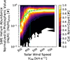 |
Fig. 1. Contour plot corresponding to a column-normalized 2D histogram of the SWE helium abundance as a function of the proton speed observed at Wind. The solid green line and error bars are the mean and standard deviation in each column. The dash-dotted pink line shows the result of a bilinear fit to the green line, where each line is selected as the minimum of both lines in the bilinear function over the full domain. Only speeds of vsw > 300 kms1 are included in the fit. Semitransparent blue lines indicate the saturation speed (vs) and saturation abundance (As) along with their uncertainties, where the bilinear function changes slope. |
To quantify this transition, we have fit the trend of these distributions with the bilinear function
![Mathematical equation: $$ \begin{aligned} A(v) = \min \left[A_1(v),A_2(v)\right] = \min \left[m_1(v - v_1), m_2 (v - v_2)\right]. \end{aligned} $$](/articles/aa/full_html/2025/02/aa51550-24/aa51550-24-eq1.gif) (1)
(1)
A(v) is the abundance normalized to its photospheric value,
 (2)
(2)
where X/H = nX/nH is the number density of species, X, normalized to the H number density. For the two lines indicated by subscript 1 or 2, Ai are the two different lines, mi are the slopes of the lines, and vi are the x intercepts of the lines. Kasper et al. (2007) calls vi for the line in Eq. (1) with the steeper slope (nominally the slow wind) the vanishing speed; that is, the speed at which AHe vanishes from the solar wind. The two lines intersect at the saturation speed (vs) at which the abundances of both lines are equal, A1 = A2 = As. The speed at the intersection between the two lines in Eq. (1) is given by
 (3)
(3)
As the intersection of two lines reduces the number of free parameters in the two equations to four, we chose to parameterize the fit function so that the free parameters are vs, As, v1 (the x intercept of the vsw < vs line), and m2 (the slope of the vsw > vs line). This parameterization directly quantifies the point at which He/H transitions from its slow to fast wind values (vs, As) and provides uncertainties for it. To account for the variable frequency with which Wind samples different solar speeds and reduce the impact of extreme values of He/H, we selected data in bins within 80% of the column maximum and then calculated the mean and standard deviation in log-space. We then fit these mean values with the minimum of two lines in Eq. (1). Each column’s standard deviation was used as the weight. The green line and error bars in Fig. 1 show the mean and standard deviation in each column. The dash-dotted pink line shows the trend. As He/H saturates to its fast wind value As = 0.530 ± 0.004 at speeds v > vs = 402 ± 2 km s−1, we refer to this as the saturation speed (vs), and the corresponding abundance as the saturation abundance (As). We refer to this coordinate (vs, As) as the “saturation point”. Although it has been suggested that this point should be referred to as a transition, that would imply the symbol vt, which could easily be confused with the thermal speed.
Solar wind acceleration and heating leave signatures in the trends of heavy ions observed at 1 AU. To characterize the impact of these signatures on the transition between slow and fast wind, we have examined the SWICS abundances of He, C, N, O, Ne, N, Mg, Si, S, and Fe, all normalized to hydrogen (X/H) in the same manner as He/H observed by SWE in Fig. 1. Figure 2 plots these SWICS and SWE abundances as a function of vsw observed at their respective spacecraft. We have limited the observations plotted to those below 600 km s−1 because Fig. 1 shows the transition is at speeds more than 100 km s−1 slower and due to large scatter at higher speeds. Every second data point is marked. Labels on the right side of the plot indicate the species, with SWE indicating He/H observed by Wind/SWE.
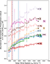 |
Fig. 2. Abundances averaged in solar wind speed bins. Saturation speeds (vs) are indicated by vertical lines of the corresponding color. The species are indicated on the right hand side of the plot. The SWE observations of AHe from Figure 1 are shown for reference in pink hexagons and labeled SWE. Only every second bin is marked for visual clarity. |
We have fit the plotted observations with the bilinear function in Eq. (1). Vertical, semitransparent lines in Fig. 2 indicate the speeds at which the slope of the bilinear fit changes; in other words, each species’ saturation speed. Table 1 gives saturation speeds (vs) and abundances (As) along with the other parameters for the fits and the percentage of the observations in the vsw < vs regime. This latter quantity shows that the slow wind portion of each species contains a nontrivial fraction of that species’ observations. Although there is more scatter in the plots due to SWICS’ lower time resolution and although the time period over which observations are available is smaller, they all show a fast-to-slow transition. Excluding He, the average heavy ion saturation speed is vs = 327 ± 2 km s−1. We have performed a similar average for the low and high FIP elements and those vs are the same to within in the propagated uncertainties. Broadly, all species show similar qualitative behavior in that all X/H monotonically increase with increasing vsw and have different gradients at speeds above and below their respective vs.
To better characterize these gradients, Fig. 3 replots the data in Fig. 2 and scales the observations to the saturation point (vs, As), which is plotted at (1, 1). He for SWE and SWICS do not extend to as large a value on the x axis as other species because vs, He is larger than vs, Heavy. This figure shows that below the saturation speed (vsw < vs), the gradient of scaled abundances as a function of vsw is indistinguishable across the different species. For speeds of vsw > vs, each species’ gradient is shallower than its vsw < vs gradient and these gradients are different for the different species. C, N, and O have the steepest gradients for vsw > vs that change the least with respect to their gradients over speeds vsw < vs. Fe and He have the shallowest gradients for speeds vsw > vs that change the most with respect to their vsw < vs gradients. Ne, Mg, Si, and S are the intermediate cases.
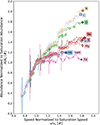 |
Fig. 3. Observations plotted in Figure 2, but scaled to their (vs, As) values, which is plotted at (1, 1). |
3.2. Saturation properties
In this section, we characterize the saturation of each species at its (vs, As) point. Figures 4, 5, and 6 use a consistent style in which each species’ color and marker match its style in Figs. 2 and 3. Data points are connected with a dotted black line to aid the eye. The top axis indicates the species. In the case of He/H from SWE, the marker is explicitly labeled to differentiate it from SWICS’ He/H.
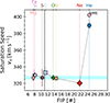 |
Fig. 4. Saturation speed (vs) as a function of the first ionization potential (FIP). The vertical dashed line is 11 eV, the nominal change between high and low FIP. The horizontal, semitransparent blue bar indicates the weighted average of vs = 327 ± 2 km s−1 for elements heavier than He. To within their mutual uncertainties, all but Ne and Si have the same vs. |
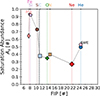 |
Fig. 5. Each element’s saturation abundance (As) as a function of FIP. The vertical dashed line is 11 eV, the nominal change between high and low FIP. The ∼2× difference between low and high FIP abundances is expected. |
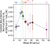 |
Fig. 6. Abundance at vsw = 592 km s−1 normalized to As as a function of the element mass. Excluding He, the decreasing trend with increasing M indicates a heavy ion fractionation process in fast solar wind. |
Figure 4 plots vs as a function of FIP. The vertical dashed line is 11 eV, the nominal change between high and low FIP (Alterman et al. 2023). It shows that vs for all heavy ions are within the 1σ fit uncertainty of each other. Ne is the exception in that the upper range of vs, Ne is slower than the lower range of vs, Si. Excluding He, the average saturation speed for heavier elements is vs = 327 ± 2 km s−1. The He/H saturation speed observed by SWICS is vs = 390 ± 4 km s−1. For comparison, vs for He/H observed by SWE is vs = 402 ± 2 km s−1, a 6 to 18 km s−1 difference, which we consider small in comparison to the 63 ± 4.5 km s−1 difference between vs for SWICS’ He/H and heavier elements.
Figure 5 plots the saturation abundance, As, as a function of FIP. Again, the vertical dashed line indicates 11 eV, the nominal transition between low and high FIP. This figure shows the expected rend that low FIP elements (FIP < 11 eV) are enhanced more than high FIP elements by a factor of approximately two. This trend is expected from Zurbuchen et al. (2016), who compared X/O in interplanetary coronal mass ejections (ICMEs), fast solar wind, and slow solar wind. That S behaves like a low FIP element is also consistent with observations of suprathermal ions during quiet times (Alterman et al. 2023).
To characterize the change in gradients for speeds vsw > vs, we have normalized the abundance at 592 km s−1 to As and plotted it as a function of element mass (M) in Fig. 6. The speed 592 km s−1 is the fastest considered in this SWICS analysis and corresponds to the filled markers in Figs. 2 and 3. Normalizing to As removes the photospheric normalization. We chose M because these quantities are not organized by FIP and several M-dependent fractionation processes have been observed (Rivera et al. 2021; Lepri & Rivera 2021; Pilleri et al. 2015; Weberg et al. 2012; Wurz et al. 2000). Table 1 includes the abundances at 592 km s−1 under A(592 km s−1). Normalizing this fastest abundance to As allows us to qualitatively characterize the gradient in a manner that accounts for the known differences in heavy ion abundances due to fractionation processes in the chromosphere and transition region (Laming 2004, 2009, 2015; Schwadron et al. 1999; Geiss 1982; Geiss et al. 1995a). Error bars are the propagated errors including the fit uncertainty in As and the statistical uncertainty in the 592 km s−1 data point. Excluding He, which is a known outlier in comparison to heavier elements, we observe a roughly monotonic decreases in A(592 km s−1)/As with three clusters. C, N, and O are clustered in the range of ∼1.8–2. Mg, Ne, Si, and S are clustered at ∼1.5. Fe’s A(592 km s−1)/As is approximately 1.2, which is comparable to He’s.
4. Discussion
Broadly, the solar wind can be classified into two types based on its speed: fast and slow. The difference between fast and slow wind is often chosen ad hoc to be somewhere in the range of 400 to 600 km s−1. For example, an oft-cited justification for classifying the solar wind as fast or slow is that the helium abundance has a strong positive gradient with solar wind speed in slow wind and saturates to a fixed value in fast wind. We have identified the speed-abundance pair at which a given element transitions from slow-wind-like to fast-wind-like behavior as (vs, As) by fitting Eq. (1) to the trends of X/H as a function of vsw. Using several solar cycles of observations from the Wind FCs, Fig. 1 shows that, statistically, He/H saturates to a photospheric-normalized abundance of As = 0.530 ± 0.004 at vs = 402 ± 2 km s−1. However, in situ observations of kinetic properties (Kasper et al. 2008, 2017; Tracy et al. 2016; Alterman et al. 2018; Klein et al. 2018; Martinović et al. 2020, 2021), chemical makeup and charge state properties (von Steiger et al. 2000; Geiss et al. 1995a,b; Zhao et al. 2017a, 2022; Xu & Borovsky 2015; Fu et al. 2017, 2015), and cross helicities (Tu & Marsch 1995; Bruno & Carbone 2013; D’Amicis et al. 2021a) indicate that the helium abundance alone carries insufficient information to fully characterize the transition between fast and slow solar wind.
We repeat the analysis in Fig. 1 for all heavy ion abundances X/H observed by ACE/SWICS, both He and heavier elements. Figure 2 plots the observations. Figure 4 summarizes the derived saturation speeds vs as a function of FIP. In the case of SWICS’ He/H, the abundance saturates to its fast wind value at vs = 390 ± 3 km s−1, which is at most 15 km s−1 slower than vs observed by Wind/SWE. Figure 4 shows that, with the exception of Ne and Si, heavy element vs are all within their mutual uncertainties. As such, we take their weighted mean vs = 327 ± 2 km s−1 as the typical heavy element saturation speed, which is indicated by a horizontal blue line in Fig. 4. This heavy ion vs is 63 ± 5 km s−1 slower than the vs observed by SWICS, which is 5× larger than the difference between vs observed by SWICS and SWE for He/H. Given that SWICS is a time-of-flight mass spectrometer, SWE consists of two FCs, and these two instruments are mounted on different spacecraft, a difference of < 4% between vs derived from SWICS and SWE measurements seems negligible in comparison to the difference between vs for He and heavier elements observed by SWICS. This suggests that SWICS and SWE observations of He/H are statistically consistent over the long duration of the observations used in this study and provides high confidence that there is not a systematic difference between these instruments that is significant on the scales statistically analyzed in this work. As such, we use the SWICS He observations for comparison with heavier element abundances.
Figure 5 plots the saturation abundance, As, the abundances at vs, as a function of FIP and shows the expected dependence. In qualitative agreement with Zurbuchen et al. (2016), Von Steiger & Zurbuchen (2016), low FIP elements are enhanced from their photospheric values by ∼2× more than high FIP elements. The agreement is qualitative because Zurbuchen et al. (2016), Von Steiger & Zurbuchen (2016) analyze X/O or normalize their X/H values to fast wind X/H, not photospheric values. The observed FIP dependence suggests the unsurprising result that the abundances characteristic of the transition between slow and fast solar wind are driven in the chromosphere, where solar wind abundances are fractionated by the ponderomotive force (Laming 2004, 2009, 2015; Schwadron et al. 1999; Geiss 1982; Geiss et al. 1995a). For completeness, we have also examined these saturation abundances as a function of element mass (M) and the typical solar wind charge state (Q) (von Steiger et al. 1997; Desai et al. 2006). Although beyond the scope of this paper and not shown for space, we note that As for high FIP elements shows a monotonic decrease with increasing M and Q.
To contextualize the gradients of X/H as a function of vsw at speeds slower and faster than vs, Fig. 3 scales the observations plotted in Fig. 2 to each species’ saturation point (vs, As). As abundances are set by FIP in the chromosphere and the solar wind’s asymptotic speed is set above this height, such a normalization removes any (simple) offsets that are due to preferential element or ion coupling to these mechanisms and reveals any trends obscured by them. This shows that in solar wind with speeds of vsw < vs, the gradients of X/H as a function of vsw are effectively indistinguishable. This is not the case for speeds of vsw > vs, for which there may be three distinct groups. For high FIP elements heavier than He (i.e., C, N, and O), the change in gradient at vsw > vs is least significant. Low FIP elements Mg, Si, and S have an intermediate change in gradient. Ne and Fe are the exceptions to this trend. Although Ne is high FIP, the change in its gradient is more similar to the low FIP elements than other high FIP elements. In the case of Fe, its gradient at vsw > vs is most similar to He, which is generally an exception to composition trends. Figure 6 plots the fastest reported abundance at 592 km s−1, the fastest speed plotted in Fig. 2 and indicated by filled markers, normalized to As as a function of mass and shows that, with the exception of He, these transition abundances As are well ordered by mass, indicating a possible mass-dependent fractionation process in solar wind with vsw > vs.
4.1. Implications for the fast–slow solar wind transition and solar wind sources
Coronal conditions are such that energy conversion at the sonic point is insufficient to yield the asymptotic fast wind speeds observed at 1 AU (Leer & Holzer 1980; Hansteen & Velli 2012). Rather, additional energy must be supplied to the solar wind to achieve the asymptotically fastest observed non-transient solar wind. In contrast to a quantity that evolves with distance like speed, elemental abundances are conserved quantities. This is key to utilizing FIP fractionation as an in situ diagnostic of solar wind source regions at the Sun. The combined measurements of abundances and speed therefore probe a combination of solar wind source region and transport effects.
The overall trends of X/H with vsw that show two distinct gradients at speeds < vs and > vs in Figs. 2 and 3 are consistent with the two-state solar wind paradigm under which fast wind is from CHs with magnetic fields that are continuously open to heliosphere and slow wind is from equatorial sources with more complex, likely intermittently open magnetic topologies. The difference between low and high FIP As in Fig. 5 is consistent with Fig. 5 in Zurbuchen et al. (2016) and a FIP-dependent process at the Sun fractionating elemental abundances in the chromosphere, which suggests that the fast–slow transition is independent of the FIP effect. Given that vs is similar for all elements heavier than He and the solar wind speed is set above heights where FIP fractionation occurs, we make the unsurprising inference that the transition between fast and slow solar wind sources occurs at heights above where the ponderomotive force or any similar process that induces fractionation impacts the solar plasma. The difference in He vs and heavy element vs along with the difference in gradients of X/H at speeds below and above vs require a more nuanced interpretation.
Two critical distances associated with solar wind acceleration are the sonic and Alfvén critical points, which we denote by rc and rA, respectively. The sonic point is the distance from the Sun’s surface at which the solar wind’s bulk speed exceeds the thermal speed. Under the Parker model (Parker 1958), this happens when the plasma’s thermal energy is converted to kinetic energy and the solar wind becomes supersonic. The Alfvén point or surface is the distance at which the solar wind’s speed exceeds the local Alfvén speed; that is, the solar wind is traveling faster than information can propagate along magnetic field lines attached to the Sun’s surface. Kasper et al. (2021) observed the Alfvén surface to be just below 20 Rs. Alfvén waves are a possible source of the energy above either rc and/or rA that is necessary for the solar wind to achieve its asymptotic fast wind values.
Our analysis assumes that there exists a characteristic point (vs, As) for each species’ abundance as a function of vsw and that this point statistically indicates a transition between measurements of plasma from CH and equatorial sources that each have characteristic speeds, abundances, and abundance gradients as a function of vsw. By normalizing the observed trends in Fig. 2 to this point (vs, As), Fig. 3 accounts for any offsets present in these trends that, by assumption, are unrelated to the process(es) that lead to the two different gradients above and below vs. Because the gradients for vsw < vs are consistent across species, we infer that there is no process that preferentially couples to and drives changes in any one species’ abundance or as a function of element properties like M, Q, M/Q, or FIP. In other words, there is no fractionation process in the slow wind beyond that which is introduced by the FIP effect in the chromosphere, as is observed by the vertical scaling in Fig. 2.
To contextualize the difference in vs for He and heavier elements, Fig. 7 plots these speeds with the probability density of vsw observations from SWICS. Vertical green lines indicate vs for He observed by SWICS and the weighted average of vs for heavier elements; line widths are the range of values covered by the uncertainties. The vertical dotted line is the peak of the vsw distribution. This visualization clearly shows that vs, He > vs, Heavy and these two characteristic speeds are separated by the solar wind distribution’s peak. Using SWE observations of vsw and He/H does not change this interpretation. That vs for elements heavier than He are mutually consistent further suggests that there is no process that preferentially accelerates heavier elements at distances from the Sun > rc or > rA, where processes that occur during transport continue to accelerate the fast solar wind to its asymptotic values. However, this does not rule out such an in situ acceleration process impacting He for vsw > vs. For example, He’s large density with respect to heavier elements makes it more likely to be impacted by beam instabilities, interparticle Coulomb collisions, and Alfvén wave transport. If the difference between vs, He and vs, Heavy is due to an in situ acceleration process at distances from the Sun above the sonic point rc preferentially coupling to He in comparison to heavier elements, the difference between vs, He and vs, Heavy has profound implications for the definitions of fast and slow solar wind.
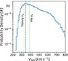 |
Fig. 7. Probability density of vsw observed by SWICS and SWE. The vertical green lines are saturation speeds vs including uncertainty. The vertical dotted black line is the peak solar wind speed bin, vsw = 345 km s−1. |
The helium abundance is a key motivator for associating fast and slow solar wind with distinct solar sources. The scaled observations in Fig. 3 show that X/H for vsw < vs have indistinguishable gradients. Figures 2 and 5 show the expected FIP fractionation. From this, we infer that observations from vsw < vs are equatorial in origin and observations from vsw > vs are CH in origin. A consequence of this is that differentiating between fast and slow solar wind with a threshold in the range of 400–600 km s−1 would yield slow wind abundances with chemical compositions reflecting a mixture of source regions continuously magnetically open to the heliosphere (e.g., CHs) and those that are only intermittently open (i.e., equatorial sources). Such mixing would obscure our ability to properly map slow solar wind back to its solar origin.
4.2. Implications for fast wind fractionation and solar wind acceleration
Pilleri et al. (2015) have studied heavy ion abundances normalized to Mg during solar minimum 23 and maximum 24 using ACE/SWICS data to contextualize Genesis observations (Burnett et al. 2003). They divide their observations into those from CHs, equatorial sources, and CMEs; calculate their abundances with respect to magnesium; and include an analysis of X/Mg’s dependence on vsw. They divide their solar wind observations into ones from CHs and ones that are equatorial in origin based on a change in solar wind speed. They report mass-dependent fractionation trends comparable to ours whereby O/Mg, C/Mg, and He/Mg show two distinct gradients above and below ∼400 km s−1, which roughly divides equatorial and CH wind. That their threshold speed is faster than the vs we report for heavy ions is unsurprising because they separate CH and equatorial solar wind by following Reisenfeld et al. (2013) and setting a threshold on solar wind speed at stream interfaces that is 425 km s−1 for rarefaction regions and 525 km s−1 compression regions. These authors also attribute their fractionation to a secondary dependence of the ponderomotive force predicted by Laming (2004). However, Laming (2004, 2009, 2015) emphasize that the ponderomotive force is effectively mass-independent. As such, another explanation may be necessary.
One possibility is that the solar wind speed varies between the center and boundary of CHs (Zhao et al. 2017a). Performing a superposed epoch analysis of 66 Carrington rotation long intervals of CH solar wind, Borovsky (2016) shows a gradient of speed in time over the range of 400–600 km s−1, which is the range over which we observe an enhancement in A(592 km s−1)/As. However, Borovsky (2016) also shows that Fe/O does not vary over these intervals. As the abundance normalized to As of Fe/H has the shallowest gradient for speeds of vsw > vs and that of O/H has one of the strongest gradients, this suggests that our observed mass fractionation is not a result of position within a CH or distance from its edge.
In the case of Coulomb friction with H dragging heavy ions out of the corona, Bodmer & Bochsler (1998, 2000) show that there is a mass dependence and the associated fractionation would be stronger in slow than fast wind. Such a trend does not agree with the fractionation we observe in fast wind and lack of fractionation in slow wind when FIP fractionation is accounted for by normalizing abundances to As. As such, we rule out Coulomb friction as a source of the observed vsw > vs trend.
Rivera et al. (2021) report signatures of mass-dependent fractionation in CMEs in which heavy ion abundances decrease with increasing mass when absolute CME abundances (X/H) are normalized to ambient absolute solar wind abundances. Lepri & Rivera (2021) report a similar trend for prominence material, though of higher values. Rivera et al. (2021) attribute this trend to gravitational settling. Weberg et al. (2012) also demonstrate that gravitational settling leads to mass-dependent fractionation in ambient solar wind. However, gravitational settling has a timescale on the order of days and requires closed loops, which are common in equatorial regions where slow wind originates, not CH regions where fast wind is from. As such, the mass-dependent fractionation observed in solar wind with speeds of vsw > vs is also unlikely due to gravitational settling.
In short, we have shown that the observed fast wind enhancements of heavy ion abundances above As and the corresponding mass-dependent fractionation are inconsistent with the effects of gravitational settling, H dragging coronal heavy ions into the solar wind by means of Coulomb friction, and gradients across CHs. Pilleri et al. (2015) suggest that mass-dependent fractionation is consistent with a ponderomotive-driven FIP effect. Although our trends qualitatively agree with Pilleri et al. (2015), Laming (2004, 2009, 2015) explicitly state that a ponderomotive-driven FIP effect is mass-independent. As such, this may be novel mass-dependent, fast wind fractionation or the fractionation may depend on a different quantity.
In addition to FIP and M, the elements reported here are summed over a series of charge states and, as such, have an average charge state. Renaud & Victoria-Feser (2010, Eq. (14)) proposed a robust coefficient of determination (Rw2) that is appropriate for rapidly determining if a model reasonably fits a set of data that includes uncertainties. Excluding He, we have fit the fastest abundances observed, A(592 km s−1)/As, as a function of FIP, M, solar wind charge state Q (von Steiger et al. 1997; Desai et al. 2006), M/Q, and M2/Q2 with a line and calculated Rw2 as a simple means of quantifying how well organized A(592 km s−1)/As is by each quantity. All Rw2 are < 0.55 except for the dependence on average charge state, for which Rw2 = 0.95. Figure 8 plots A(592 km s−1)/As as a function of the charge state in the style of Figs. 4 and 6. Although we do not have an explanation for this result, it suggests that the fractionation may depend on the solar wind charge state.
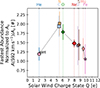 |
Fig. 8. Abundance at vsw = 592 km s−1 normalized to As as a function of the solar wind charge state. Excluding He, the decreasing trend with increasing M indicates a heavy ion fractionation process in fast solar wind. |
Beyond the reported M- or Q-dependent fractionation of A(vsw > vs)/As, Fig. 3 shows that the degree of fractionation increases with vsw for vsw > vs. To achieve the asymptotically fastest speeds observed at 1 AU, energy must be deposited into the solar wind above the sonic critical point rc (Leer & Holzer 1980; Hansteen & Velli 2012). The faster the speed before this yet-to-be-identified mechanism accelerates the solar wind and the more energy that is deposited by it, the larger the asymptotic speed. Recent work (Rivera et al. 2024b; Bale et al. 2023; Raouafi et al. 2023) shows that the solar wind’s acceleration at distances of r > rA is driven by the deposition of energy into the solar wind from switchback dissipation during solar wind propagation through interplanetary space. Given that all ions observed at fast wind speeds, which the solar wind requires such energy deposition to reach, the increase in the degree of heavy ion fractionation may indicate that there is a preferential coupling between these heavy ions and the energy deposition process. On the other hand, we have argued that the consistency of vs across the heavy ions suggests that vs, He > vs, Heavy may indicate He is impacted by this yet-to-be-identified acceleration mechanism at distances from the sun above rc and heavier elements are not. If this is the case, then the dependence of the fractionation process for vsw > vs must be located at or near rc.
5. Conclusion
Under the two-state paradigm, the solar wind is classified into fast and slow based on whether its speed is above or below a threshold value. This threshold is typically between ∼400 and ∼600 km s−1 and chosen in an ad hoc or heuristic fashion. Fast solar wind with speeds above this threshold value is typically observed to come from magnetically open regions, typically polar regions like CHs (Phillips et al. 1994; Geiss et al. 1995b). Slow solar wind is from more equatorial regions with magnetic fields that may only be intermittently open to the heliosphere (Fisk et al. 1999; Subramanian et al. 2010; Antiochos et al. 2011; Crooker et al. 2012; Abbo et al. 2016; Antonucci et al. 2005). Analysis of the solar wind’s kinetic (Kasper et al. 2008, 2017; Tracy et al. 2016; Kasper et al. 2006; Fu et al. 2018; Stakhiv et al. 2016; Alterman et al. 2018), heavy ion abundance along with the charge-state ratio (von Steiger et al. 2000; Geiss et al. 1995b,a; Zhao et al. 2017a, 2022; Xu & Borovsky 2015; Fu et al. 2017, 2015), Alfvénicity (D’Amicis et al. 2021b; D’Amicis et al. 2021a; Bruno & Carbone 2013; Tu & Marsch 1995), and heavy ion composition in switchbacks (Rivera et al. 2024a) provide a more nuanced picture in which there are multiple classes of solar wind.
Motivated by the distinct gradients of He/H as a function of vsw observed by Wind/SWE above and below the speed vs, we have investigated the variation in X/H observed by ACE/SWICS as a function of vsw. We have made the following observations and inferences.
-
All species have two distinct gradients as a function of vsw and these gradients are shallower above the speed vs. From this, we infer that the change in gradients is a signature of differences in the magnetic topology at distinct types of solar wind source regions.
-
The He saturation speed is vs = 402 ± 2 km s−1 (observed by SWE) and vs = 390 ± 4 km s−1 (observed by SWICS). We interpret this as showing that SWE and SWICS He/H are statistically consistent over the years 1998 to 2011.
-
The average vs across elements heavier than He is vs = 327 ± 2 km s−1, independent of species, which is 63 ± 4.5 km s−1 slower than vs for SWICS’ He/H. Moreover, the speed, vs, of heavy elements is slower than the peak of the solar wind distribution and the speed vs of He is faster than the peak of the solar wind distribution. From this, we infer that He may be impacted by the acceleration at heights above the sonic point that is necessary for non-transient solar wind to reach the asymptotically fastest speeds observed at 1 AU and heavy elements are not.
-
If our inferences about the change in gradients of X/H as a function of vsw across vs and the observation that vs, He > vs, Heavy hold, then this implies that setting a threshold for differentiating between slow and fast solar wind in the range of 400–600 km s−1 may lead to a slow solar wind with a chemical makeup that is a mixture of solar wind from CH and equatorial regions that are only intermittently open to the heliosphere.
-
The saturation abundances (As) are ordered by FIP and show an expected fast wind fractionation pattern. From this, we unsurprisingly infer that the fast–slow solar wind transition is the result of a mechanism that impacts the solar wind at heights above chromosphere, above where processes like the ponderomotive force that would fractionates the solar plasma occur.
-
When normalized to the point (vs, As) the gradients of elements heavier than He are indistinguishable for vsw < vs. We interpret this observation as a signature that there is not a mechanism preferentially coupled to and driving slow wind abundance gradients as a function of species.
-
When normalized to the point (vs, As) the gradients of elements heavier than He for vsw > vs are ordered by M or average solar wind Q. Although the average charge state provides a better ordering of the ratio of the fastest reported abundances to the saturation abundances A(592 km s−1)/As, as is indicated by the weighted coefficient of determination, such a fractionation process that only depends on the average charge state is difficult to justify. Even though we have ruled out multiple mass-dependent mechanisms as possible sources of the observed fractionation at speeds vsw > vs, this renders such a charge-state-dependent fractionation unsatisfying.
The bimodal nature of the solar wind’s distribution is most pronounced during solar minima when CHs are restricted to the Sun’s polar regions and its equatorial regions are dominated by helmet streamers, pseudostreamers, and other features with magnetic topologies that are not connected to the heliosphere in a simple, radial fashion. Furthermore, additional properties like the solar wind’s Alfvénicity have shown that there is solar wind with speeds that are traditionally considered to be slow, but fast wind kinetic, chemical, and charge state properties. This Alfvénic slow wind is believed to emanate from CHs and not equatorial sources. Further analysis of the solar wind’s chemical makeup and its variation as a function of Alfvénicity and solar activity should provide additional insights into the relationship between in situ solar wind observations and their sources on the Sun.
Acknowledgments
The authors thank Ruth Skoge for discussions of ACE/SWEPAM data. BLA acknowledges NASA Grants 80NSSC22K0645 (LWS/TM), 80NSSC22K1011 (LWS), and 80NSSC20K1844. YJR acknowledges support from the Future Faculty Leaders postdoctoral fellowship at Harvard University. JMR and STL acknowledge NASA contract 80NSSC23K0542 (ACE/SWICS).
References
- Abbo, L., Ofman, L., Antiochos, S. K., et al. 2016, Space Sci. Rev., 201, 55 [NASA ADS] [CrossRef] [Google Scholar]
- Acuña, M. H., Ogilvie, K. W., Baker, D. N., et al. 1995, Space Sci. Rev., 71, 5 [Google Scholar]
- Aellig, M. R., Lazarus, A. J., & Steinberg, J. T. 2001, GRL, 28, 2767 [NASA ADS] [CrossRef] [Google Scholar]
- Alterman, B. L., & Kasper, J. C. 2019, ApJ, 879, L6 [Google Scholar]
- Alterman, B. L., Kasper, J. C., Stevens, M., & Koval, A. 2018, ApJ, 864, 112 [NASA ADS] [CrossRef] [Google Scholar]
- Alterman, B. L., Kasper, J. C., Leamon, R. J., & McIntosh, S. W. 2021, Sol. Phys., 296, 67 [Google Scholar]
- Alterman, B. L., Desai, M. I., Dayeh, M. A., Mason, G. M., & Ho, G. 2023, ApJ, 952, 42 [NASA ADS] [CrossRef] [Google Scholar]
- Antiochos, S. K., Mikic, Z., Titov, V. S., Lionello, R., & Linker, J. A. 2011, ApJ, 731, 112 [NASA ADS] [CrossRef] [Google Scholar]
- Antonucci, E., Abbo, L., & Dodero, M. A. 2005, A&A, 435, 699 [NASA ADS] [CrossRef] [EDP Sciences] [Google Scholar]
- Asplund, M., Amarsi, A. M., & Grevesse, N. 2021, A&A, 653, A141 [NASA ADS] [CrossRef] [EDP Sciences] [Google Scholar]
- Baker, D., Démoulin, P., Yardley, S. L., et al. 2023, ApJ, 950, 65 [CrossRef] [Google Scholar]
- Bale, S. D., Drake, J. F., McManus, M. D., et al. 2023, Nature, 618, 252 [NASA ADS] [CrossRef] [Google Scholar]
- Bodmer, R., & Bochsler, P. 1998, Phys. Chem. Earth, 23, 683 [NASA ADS] [CrossRef] [Google Scholar]
- Bodmer, R., & Bochsler, P. 2000, J. Geophys. Res.: Space Phys., 105, 47 [NASA ADS] [CrossRef] [Google Scholar]
- Borovsky, J. 2016, JGR A: Space Phys., 121, 5055 [Google Scholar]
- Brooks, D. H., Ugarte-Urra, I., & Warren, H. P. 2015, Nat. Commun., 6, 5947 [Google Scholar]
- Bruno, R., & Carbone, V. 2013, Liv. Rev. Sol. Phys., 10, 1 [Google Scholar]
- Burnett, D. S., Barraclough, B. L., Bennett, R., et al. 2003, Space Sci. Rev., 105, 509 [CrossRef] [Google Scholar]
- Crooker, N. U., Antiochos, S. K., Zhao, X., & Neugebauer, M. 2012, J. Geophys. Res.: Space Phys., 117, A4 [NASA ADS] [Google Scholar]
- D’Amicis, R., & Bruno, R. 2015, ApJ, 805, 1 [NASA ADS] [CrossRef] [Google Scholar]
- D’Amicis, R., Alielden, K., Perrone, D., et al. 2021a, A&A, 654, A111 [NASA ADS] [CrossRef] [EDP Sciences] [Google Scholar]
- D’Amicis, R., Perrone, D., Bruno, R., & Velli, M. 2021b, J. Geophys. Res.: Space Phys., 126, e2020JA028996 [Google Scholar]
- Del Zanna, G. 2019, A&A, 624, A36 [NASA ADS] [CrossRef] [EDP Sciences] [Google Scholar]
- Desai, M., Mason, G., Gold, R. E., et al. 2006, ApJ, 649, 470 [NASA ADS] [CrossRef] [Google Scholar]
- Doschek, G. A., & Warren, H. P. 2019, ApJ, 884, 158 [Google Scholar]
- Du, Z. 2012, Sol. Phys., 278, 203 [NASA ADS] [CrossRef] [Google Scholar]
- Feldman, U., & Laming, J. M. 2000, Phys. Scr., 61, 222 [NASA ADS] [CrossRef] [Google Scholar]
- Feldman, W. C., Asbridge, J. R., Bame, S. J., & Gosling, J. T. 1978, J. Geophys. Res., 83, 2177 [NASA ADS] [CrossRef] [Google Scholar]
- Fisk, L. A., Zurbuchen, T. H., & Schwadron, N. A. 1999, ApJ, 521, 868 [Google Scholar]
- Fu, H., Li, B., Li, X., et al. 2015, Sol. Phys., 290, 1399 [CrossRef] [Google Scholar]
- Fu, H., Madjarska, M. S., Xia, L., et al. 2017, ApJ, 836, 169 [Google Scholar]
- Fu, H., Madjarska, M. S., Li, B., Xia, L., & Huang, Z. 2018, MNRAS, 478, 1884 [CrossRef] [Google Scholar]
- Geiss, J. 1982, Space Sci. Rev., 33, 201 [Google Scholar]
- Geiss, J., Gloeckler, G., & von Steiger, R. 1995a, Space Sci. Rev., 72, 49 [NASA ADS] [CrossRef] [Google Scholar]
- Geiss, J., Gloeckler, G., Von Steiger, R., et al. 1995b, Science, 268, 1033 [CrossRef] [Google Scholar]
- Gloeckler, G., Cain, J., Ipavich, F. M., et al. 1998, Space Sci. Rev., 86, 497 [NASA ADS] [CrossRef] [Google Scholar]
- Hansteen, V. H., & Velli, M. 2012, Space Sci. Rev., 172, 89 [Google Scholar]
- Hathaway, D. H. 2015, Liv. Rev. Sol. Phys., 12, 4 [Google Scholar]
- Hewins, I. M., Gibson, S. E., Webb, D. F., et al. 2020, Sol. Phys., 295, 161 [Google Scholar]
- Hirshberg, J. 1973, Rev. Geophys., 11, 115 [NASA ADS] [CrossRef] [Google Scholar]
- Holzer, T. E., & Leer, E. 1980, J. Geophys. Res.: Space Phys., 85, 4665 [CrossRef] [Google Scholar]
- Holzer, T. E., & Leer, E. 1981, Solar Wind 4 (Burhausen, Germany: Max Planck Institut für Aeronomie and Max Planck Institut für exraterrestriesche Physik), 28 [Google Scholar]
- Johnson, M., Rivera, Y. J., Niembro, T., et al. 2024, ApJ, 964, 81 [Google Scholar]
- Johnstone, C. P., Güdel, M., Lüftinger, T., Toth, G., & Brott, I. 2015, A&A, 577, A27 [NASA ADS] [CrossRef] [EDP Sciences] [Google Scholar]
- Kasper, J. C. 2002, Ph.D. Thesis, Massachusetts Institute of Technology, USA [Google Scholar]
- Kasper, J. C., Lazarus, A. J., Steinberg, J. T., Ogilvie, K. W., & Szabo, A. 2006, J. Geophys. Res., 111, A03105 [NASA ADS] [CrossRef] [Google Scholar]
- Kasper, J. C., Stevens, M., Lazarus, A. J., Steinberg, J. T., & Ogilvie, K. W. 2007, ApJ, 660, 901 [NASA ADS] [CrossRef] [Google Scholar]
- Kasper, J. C., Lazarus, A. J., & Gary, S. P. 2008, Phys. Rev. Lett., 101, 261103 [Google Scholar]
- Kasper, J. C., Stevens, M. L., Korreck, K. E., et al. 2012, ApJ, 745, 162 [Google Scholar]
- Kasper, J. C., Klein, K. G., Weber, T., et al. 2017, ApJ, 849, 126 [NASA ADS] [CrossRef] [Google Scholar]
- Kasper, J. C., Klein, K. G., Lichko, E., et al. 2021, Phys. Rev. Lett., 127, 255101 [NASA ADS] [CrossRef] [Google Scholar]
- Klein, K. G., Alterman, B. L., Stevens, M., Vech, D., & Kasper, J. C. 2018, Phys. Rev. Lett., 120, 205102 [NASA ADS] [CrossRef] [Google Scholar]
- Laming, J. M. 2004, ApJ, 614, 1063 [Google Scholar]
- Laming, J. M. 2009, ApJ, 695, 954 [NASA ADS] [CrossRef] [Google Scholar]
- Laming, J. M. 2012, ApJ, 744, 115 [NASA ADS] [CrossRef] [Google Scholar]
- Laming, J. M. 2015, Liv. Rev. Sol. Phys., 12, 2 [Google Scholar]
- Leer, E., & Holzer, T. E. 1980, J. Geophys. Res.: Space Phys., 85, 4681 [NASA ADS] [CrossRef] [Google Scholar]
- Lepri, S. T., & Rivera, Y. J. 2021, ApJ, 912, 51 [NASA ADS] [CrossRef] [Google Scholar]
- Lepri, S. T., Landi, E., & Zurbuchen, T. H. 2013, ApJ, 768, 94 [NASA ADS] [CrossRef] [Google Scholar]
- Livi, S. A., Lepri, S. T., Raines, J. M., Dewey, R., et al. 2023, A&A, 676, A36 [NASA ADS] [CrossRef] [EDP Sciences] [Google Scholar]
- Marsch, E. 2006, Adv. Space Res., 38, 921 [NASA ADS] [CrossRef] [Google Scholar]
- Martinović, M., Klein, K. G., Kasper, J. C., et al. 2020, ApJS, 246, 30 [CrossRef] [Google Scholar]
- Martinović, M., Klein, K. G., Durovcova, T., & Alterman, B. L. 2021, Ion-Driven Instabilities in the Inner Heliosphere I: Statistical Trends, 923, 116 [Google Scholar]
- Maruca, B. A., & Kasper, J. C. 2013, Adv. Space Res., 52, 723 [NASA ADS] [CrossRef] [Google Scholar]
- Mason, G. M., Desai, M., & Li, G. 2012, ApJ, 748, L2010 [Google Scholar]
- McComas, D. J., Ebert, R. W., Elliott, H. A., et al. 2008, Geophysical Research Lett., 35, L18103 [NASA ADS] [Google Scholar]
- McIntosh, S. W., Kiefer, K. K., Leamon, R. J., Kasper, J. C., & Stevens, M. 2011, ApJ, 740, L1 [Google Scholar]
- McIntosh, S. W., Leamon, R. J., Krista, L. D., et al. 2015, Nat. Commun., 6, 1 [CrossRef] [Google Scholar]
- Meyer-Vernet, N. 2007, Basics of the Solar Wind, 1st edn. (Cambridge University Press) [Google Scholar]
- Mihailescu, T., Brooks, D. H., Laming, J. M., et al. 2023, ApJ, 959, 72 [Google Scholar]
- Nicolaou, G., Livadiotis, G., & Moussas, X. 2014, Sol. Phys., 289, 1371 [NASA ADS] [CrossRef] [Google Scholar]
- Ogilvie, K. W., Chornay, D. J., Fritzenreiter, R. J., et al. 1995, Space Sci. Rev., 71, 55 [Google Scholar]
- Parker, E. N. 1958, ApJ, 128, 664 [Google Scholar]
- Phillips, J. L., Balogh, A., Bame, S. J., et al. 1994, Geophys. Res. Lett., 21, 1105 [NASA ADS] [CrossRef] [Google Scholar]
- Pilleri, P., Reisenfeld, D. B., Zurbuchen, T. H., et al. 2015, ApJ, 812, 1 [NASA ADS] [CrossRef] [Google Scholar]
- Pottasch, S. R. 1963, ApJ, 137, 945 [NASA ADS] [CrossRef] [Google Scholar]
- Raouafi, N. E., Stenborg, G., Seaton, D. B., et al. 2023, ApJ, 945, 28 [NASA ADS] [CrossRef] [Google Scholar]
- Raymond, J. C., Kohl, J. L., Noci, G., et al. 1997, in The First Results from SOHO, eds. B. Fleck, & Z. Švestka (Dordrecht: Springer, Netherlands), 645 [CrossRef] [Google Scholar]
- Reisenfeld, D. B., Wiens, R. C., Barraclough, B. L., et al. 2013, Space Sci. Rev., 175, 125 [CrossRef] [Google Scholar]
- Renaud, O., & Victoria-Feser, M.-P. 2010, J. Stat. Plan. Inference, 140, 1852 [CrossRef] [Google Scholar]
- Richardson, I. G., & Cane, H. V. 2010, Sol. Phys., 264, 189 [NASA ADS] [CrossRef] [Google Scholar]
- Rivera, Y. J., Landi, E., Lepri, S. T., & Gilbert, J. A. 2020, ApJ, 899, 11 [Google Scholar]
- Rivera, Y. J., Lepri, S. T., Raymond, J. C., et al. 2021, ApJ, 921, 93 [CrossRef] [Google Scholar]
- Rivera, Y. J., Higginson, A., Lepri, S. T., et al. 2022a, Front. Astron. Space Sci., 9, 1056347 [CrossRef] [Google Scholar]
- Rivera, Y. J., Raymond, J. C., Landi, E., et al. 2022b, ApJ, 936, 83 [NASA ADS] [CrossRef] [Google Scholar]
- Rivera, Y. J., Badman, S. T., Stevens, M. L., et al. 2024a, ApJ, 974, 198 [NASA ADS] [CrossRef] [Google Scholar]
- Rivera, Y. J., Badman, S. T., Stevens, M. L., et al. 2024b, Science, 385, 962 [NASA ADS] [CrossRef] [Google Scholar]
- Schwadron, N. A., Fisk, L. A., & Zurbuchen, T. H. 1999, ApJ, 521, 859 [Google Scholar]
- Schwenn, R. 2006, Space Sci. Rev., 124, 51 [Google Scholar]
- Shearer, P., von Steiger, R., Raines, J. M., et al. 2014, ApJ, 789, 60 [NASA ADS] [CrossRef] [Google Scholar]
- Song, H. Q., Zhang, J., Cheng, X., et al. 2020, ApJ, 901, L21 [NASA ADS] [CrossRef] [Google Scholar]
- Stakhiv, M. O., Landi, E., Lepri, S. T., Oran, R., & Zurbuchen, T. H. 2015, ApJ, 801, 100 [NASA ADS] [CrossRef] [Google Scholar]
- Stakhiv, M. O., Lepri, S. T., Landi, E., Tracy, P. J., & Zurbuchen, T. H. 2016, ApJ, 829, 117 [NASA ADS] [CrossRef] [Google Scholar]
- Stone, E. C., Frandsen, A. M., Mewaldt, R. A., et al. 1998, Space Sci. Rev., 86, 1 [Google Scholar]
- Subramanian, S., Madjarska, M. S., & Doyle, J. G. 2010, A&A, 516, A50 [NASA ADS] [CrossRef] [EDP Sciences] [Google Scholar]
- Tlatov, A., Tavastsherna, K., & Vasil’eva, V. 2014, Sol. Phys., 289, 1349 [Google Scholar]
- Tracy, P. J., Kasper, J. C., Raines, J. M., et al. 2016, Phys. Rev. Lett., 255101, 255101 [CrossRef] [Google Scholar]
- Tu, C. Y., & Marsch, E. 1995, Space Sci. Rev., 73, 1 [Google Scholar]
- Verscharen, D., Klein, K. G., & Maruca, B. A. 2019, The Multi-scale Nature of the Solar Wind (Springer International Publishing), 16 [Google Scholar]
- Viall, N. M., & Borovsky, J. 2020, J. Geophys. Res.: Space Phys., 125, 1 [Google Scholar]
- Von Steiger, R., & Zurbuchen, T. H. 2016, ApJ, 816, 13 [Google Scholar]
- von Steiger, R., Geiss, J., & Gloeckler, G. 1997, in Cosmic Winds and the Heliosphere, Space Science Series, 581 [Google Scholar]
- von Steiger, R., Schwadron, N. A., Fisk, L. A., et al. 2000, J. Geophys. Res.: Space Phys., 105, 27217 [Google Scholar]
- Wang, Y. M., & Sheeley, N. R. 2002, J. Geophys. Res.: Space Phys., 107, 1 [NASA ADS] [CrossRef] [Google Scholar]
- Weberg, M. 2015, Spatial and Temporal Coordinate Systems in Space Physics, Tech. rep [Google Scholar]
- Weberg, M., Zurbuchen, T. H., & Lepri, S. T. 2012, ApJ, 760, 30 [Google Scholar]
- Widing, K. G., & Feldman, U. 2001, ApJ, 555, 426 [Google Scholar]
- Wurz, P., Bochsler, P., & Lee, M. A. 2000, J. Geophys. Res.: Space Phys., 105, 27239 [NASA ADS] [CrossRef] [Google Scholar]
- Xu, F., & Borovsky, J. 2015, J. Geophys. Res.: Space Phys., 120, 70 [NASA ADS] [CrossRef] [Google Scholar]
- Yogesh, C. D., & Srivastava, N. 2021, MNRAS, 503, L17 [NASA ADS] [CrossRef] [Google Scholar]
- Yogesh, C. D., & Srivastava, N. 2023, MNRAS, 526, L13 [NASA ADS] [Google Scholar]
- Zerbo, J.-L., & Richardson, J. D. 2015, J. Geophys. Res.: Space Phys., 120, 10,250 [NASA ADS] [CrossRef] [Google Scholar]
- Zhao, L., Landi, E., Lepri, S. T., et al. 2017a, ApJ, 846, 135 [Google Scholar]
- Zhao, L., Zhang, M., & Rassoul, H. K. 2017b, ApJ, 836, 31 [NASA ADS] [CrossRef] [Google Scholar]
- Zhao, L., Landi, E., Lepri, S. T., & Carpenter, D. 2022, Universe, 8, 393 [NASA ADS] [CrossRef] [Google Scholar]
- Zurbuchen, T. H., & Richardson, I. G. 2006, Space Sci. Rev., 123, 31 [Google Scholar]
- Zurbuchen, T. H., Weberg, M., Von Steiger, R., et al. 2016, ApJ, 826, 10 [CrossRef] [Google Scholar]
All Tables
All Figures
|
Fig. 1. Contour plot corresponding to a column-normalized 2D histogram of the SWE helium abundance as a function of the proton speed observed at Wind. The solid green line and error bars are the mean and standard deviation in each column. The dash-dotted pink line shows the result of a bilinear fit to the green line, where each line is selected as the minimum of both lines in the bilinear function over the full domain. Only speeds of vsw > 300 kms1 are included in the fit. Semitransparent blue lines indicate the saturation speed (vs) and saturation abundance (As) along with their uncertainties, where the bilinear function changes slope. |
| In the text | |
|
Fig. 2. Abundances averaged in solar wind speed bins. Saturation speeds (vs) are indicated by vertical lines of the corresponding color. The species are indicated on the right hand side of the plot. The SWE observations of AHe from Figure 1 are shown for reference in pink hexagons and labeled SWE. Only every second bin is marked for visual clarity. |
| In the text | |
|
Fig. 3. Observations plotted in Figure 2, but scaled to their (vs, As) values, which is plotted at (1, 1). |
| In the text | |
|
Fig. 4. Saturation speed (vs) as a function of the first ionization potential (FIP). The vertical dashed line is 11 eV, the nominal change between high and low FIP. The horizontal, semitransparent blue bar indicates the weighted average of vs = 327 ± 2 km s−1 for elements heavier than He. To within their mutual uncertainties, all but Ne and Si have the same vs. |
| In the text | |
|
Fig. 5. Each element’s saturation abundance (As) as a function of FIP. The vertical dashed line is 11 eV, the nominal change between high and low FIP. The ∼2× difference between low and high FIP abundances is expected. |
| In the text | |
|
Fig. 6. Abundance at vsw = 592 km s−1 normalized to As as a function of the element mass. Excluding He, the decreasing trend with increasing M indicates a heavy ion fractionation process in fast solar wind. |
| In the text | |
|
Fig. 7. Probability density of vsw observed by SWICS and SWE. The vertical green lines are saturation speeds vs including uncertainty. The vertical dotted black line is the peak solar wind speed bin, vsw = 345 km s−1. |
| In the text | |
|
Fig. 8. Abundance at vsw = 592 km s−1 normalized to As as a function of the solar wind charge state. Excluding He, the decreasing trend with increasing M indicates a heavy ion fractionation process in fast solar wind. |
| In the text | |
Current usage metrics show cumulative count of Article Views (full-text article views including HTML views, PDF and ePub downloads, according to the available data) and Abstracts Views on Vision4Press platform.
Data correspond to usage on the plateform after 2015. The current usage metrics is available 48-96 hours after online publication and is updated daily on week days.
Initial download of the metrics may take a while.